U.S. Department of Transportation
Federal Highway Administration
1200 New Jersey Avenue, SE
Washington, DC 20590
202-366-4000
Federal Highway Administration Research and Technology
Coordinating, Developing, and Delivering Highway Transportation Innovations
 |
| This report is an archived publication and may contain dated technical, contact, and link information |
|
Publication Number: FHWA-HRT-04-140
Date: December 2005 |
||||||||||||||||||||||||||||||||||||||||||||||||||||||||||||||||||||||||||||||||||||||||||||||||||||||||||||||||||||||||||||||||||||||||||||||||||||||||||||||||||||||||||||||||||||||||
Enhanced Night Visibility Series, Volume IX: Phase II—Characterization of Experimental ObjectsPDF Version (716 KB)
PDF files can be viewed with the Acrobat® Reader® CHAPTER 4—DISCUSSIONThe measurement results show several different analyses of photometric data obtained for all of the objects with all of the VESs. To relate these results to those of the ENV visual performance testing, the metrics calculated here must be related to the measured visibility distances from the ENV clear-condition study. To answer the research questions, the data for both the visual performance and the object characterization studies have been combined to provide an analysis of the most suitable photometric performance indicator or object detection and recognition and the threshold values obtained for the measurements. For details on the visual performance measurements, please refer to ENV Volume III, Visual Performance During Nighttime Driving in Clear Weather. Following is a list of the research questions posed for this investigation and a discussion of the findings. What is the correlation between the photometric performance of the VESs and the visual detection and recognition performance from the ENV visual performance studies? The correlation of the visual performance results with those of the photometric characterization was performed using a Pearson correlation method. In this process, the correlation coefficients for the detection and recognition distance results were calculated for the object luminance, background luminance, luminance difference, contrast, and VL. The parallel pedestrian data was used to represent the correlations relating to the static pedestrian because the photometric characterizations of those two pedestrian objects were the same. The data for the IR–TIS VES were not included in the correlation calculation because this VES is based on a camera system that was not photometrically analyzed. In addition to contrast as defined earlier, another formulation of contrast was used in this correlation analysis. This is the Weber ratio, shown in figure 62, which typically is used for complex images. In this case, the positive and negative aspect of the relationship is removed, and the maximum and minimum luminance values are used. Figure 62. Equation. Weber ratio contrast equation.
For all conditions of age, VES, and object type, the Pearson correlation coefficient was calculated between the detection and recognition distance and all of the photometric measures at 61.0 m (200 ft). This distance was used because it generally represents the performance of the metrics at all distances as shown in the results. The correlation results are shown in table 8.
In this table, the results show detection distance correlation coefficient values of between 0.596 and 0.673 for all the metrics but background luminance. Similarly, the range of correlation coefficients for the recognition distance is 0.576 to 0.658, with the Weber ratio as the highest value. Because the background luminance shows no relationship to the data, it will not be considered further. Also, because the results for the detection and recognition distance are similar and the detection of objects is more important for driver safety, only the detection distance will be considered further. In the next correlation analysis, participant age was considered separately. The results for the correlation analysis by age are shown in table 9. These results show that all of the Pearson r correlation coefficients are within approximately the same range, and the Weber ratio shows the highest correlation to the detection distance results for each age group. In general, the correlations are similar between the different age groups for all of the metrics.
The next analysis was the correlation of the detection distances and the photometric variables by the object type. The correlation results for the cyclist, parallel pedestrian, perpendicular pedestrian, static pedestrian, child’s bicycle, and tire tread are shown in table 10. The results for the cyclist, perpendicular pedestrian, and parallel pedestrian are all relatively high. In each of these object types, the Weber ratio performs the best and the VL performs the worst. The correlation values for the static pedestrian, child’s bicycle, and tire tread are very low, showing that the visual performance results are not strongly related to the photometric results for these objects. Their poor performance may be a result of these objects being located at the side of the road, but this effect was not evident for the parallel pedestrian; however, the background pavement marking came into play for these objects, and it may have influenced their visibility from the moving vehicle. The visual performance study’s parallel pedestrian was dynamic, and the other objects in this location were stationary, which may have made it more easily seen and more highly correlated to the photometric measurements.
The final aspect of the correlation analysis is the correlation by the VES type, shown in table 11. The results of the analysis show that either the object luminance or the Weber ratio had the highest correlation to the visibility distance results; the VL or the contrast had the lowest. Generally, the relationships are in the same range for all of the VES types, with the HHB values being the highest overall and the five UV–A + HID values being the lowest. For the HLB-based VESs, the addition of UV–A to the system seemed to maintain the same levels of correlation as those of the HLB baseline, whereas the addition of UV–A to the HID-based VESs seemed to degrade their correlations. This effect might be a result of two issues. The first is the cutoff of the light distribution pattern because the HLB did not have a cutoff and the HID did. The second might be the aiming issues mentioned previously. Because the UV–A sources were aimed directly in front of the vehicle, it would be expected that the cutoff area of the light source would be filled in by the UV–A emission, which may affect the correlation performance.
From the correlation analysis, it appears that the Weber ratio may be the measure most highly correlated to the detection distance. This appears to be true for all of the objects, ages, and VESs investigated. The other metrics also performed well and showed a reasonable correlation to the results. The VL, which in general performed the worst, still had a mean correlation coefficient of 0.556 as compared to 0.651 for the Weber ratio. Based on these results, it is likely that any of the metrics would provide an equally adequate representation of the visibility distance. Of the visibility metrics analyzed, what threshold values are required for the detection and recognition of the objects tested? The threshold is the point at which the participant detected the object, and the threshold value is the value of the metric when this occurred. For this aspect of the analysis, the threshold values were calculated from the distance relationships shown earlier in the photometric data results. Linear interpolation was used to estimate the parameter values at the midpoints between successive measurement distances. That is to say, if a participant had a detection or recognition distance of 183 m (600 ft), the threshold value was determined by linear interpolation between the 152.5-m (500-ft) and 244-m (800-ft) photometric measurements. This calculation was performed for all of the calculated and measured metrics. Because the photometric performance data is in the range of 61.0 m (200 ft) to 244 m (800 ft), any detection or recognition performed by a participant outside of these limits was not used in this analysis. In terms of visual object detection, there are two laws that define the threshold of vision and the photometric conditions at that threshold contrast. The first is Ricco’s law, which states that the product of the luminance of an object and the visual or angular size of the object is a constant. This means that the smaller the angular size of an object, the more luminous the surface must be to be seen. This relationship holds until a certain angular size is met, at which point the addition of more luminance will not make the object any more visible. After the object reaches this critical size, Weber’s law is evident; the size no longer contributes to the detectability of the object, and the threshold contrast is determined only by the magnitude of the background luminance. The critical size at which an object changes between the Ricco relationship and the Weber relationship defines the limit of human spatial-visual summation, and it is called the Ricco area. According to Hood and Finkelstein, the Ricco area is on the order of 6 minutes of arc.(3) Using this value, a critical distance can be calculated that defines the point where the visual angle of the object is large enough to make Ricco’s law unusable and make Weber’s law the dominant visual relationship. These distances have been calculated for the objects in this investigation, shown in table 12.
For any object with a detection distance shorter than the critical distance, where Weber’s law dominates, it would be expected that during the object detection task the object would be visible to the participant when a certain combination of object luminance and background luminance was reached. The object size is not critical within this distance, and the threshold values should be the same for all the conditions of object and VES. For objects outside of this critical distance, the threshold values should increase with the visual size of the object. The threshold values for the Weber ratio, which was the highest-performing metric in the correlation analysis, are presented in figure 63 for the black-clothed objects and figure 64 for the white-clothed objects. It should be noted that for brevity, only the data for the older participants are presented here because this age group had the highest number of detection data points within the required distance range. Because the critical distance for these pedestrian and cyclist objects is 238 m (781 ft), which is close to the limit of the measurements, all of the objects in this figure would be expected to be based on Weber’s law, so the resulting threshold values should be close to equivalent. It appears from the figure that this is generally true. This is particularly true of the white-clothed objects; there are no significant differences among their Weber ratios for the VESs, with the exception of the UV–A + HID combinations. 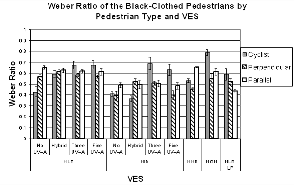 Figure 63. Bar graph. Threshold Weber ratio for black-clothed pedestrian objects.
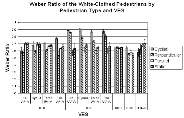 Figure 64. Bar graph. Threshold Weber ratio for white-clothed pedestrian objects.
One of the limitations of the Weber contrast ratio is that visual object size is not a component of its calculation. This results in the use of the critical distance to define the expected behavior of the relationship; however, the VL is designed to account for both Ricco’s and Weber’s laws. Although the VL metric was generally the least correlated to the detection and recognition results, consideration of the threshold values provides some interesting insight into the VL results. It would be expected that the threshold values would result in the same VL. The threshold VL values for the black-clothed objects are shown in figure 65. It is interesting that the values are not consistent across all of the VESs; however, for the HHB, HOH, HLB–LP, and HLB-based VESs, they appear to be very similar to each other. The addition of the UV–A to the HID-based VESs appears to cause some variation, which is interesting because the earlier analysis showed that the UV–A should have no effect on the black-clothed objects. Another interesting result is that of the black-clothed cyclist. Most of the threshold values for the black-clothed cyclist are close to or below 1, where the object should be invisible, indicating that the shiny rims of the bicycles were the key to the visibility of those objects, not the cyclists themselves. The final aspect of note in this figure is that the threshold value ranges between 2 and 4 for pedestrians with the exception of the cyclist and the HID-based VESs. This is consistent with the recommendations of the IESNA RP-8-00.(2) 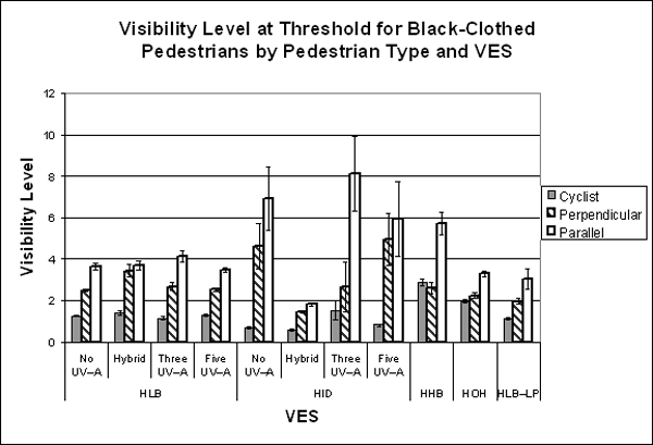 Figure 65. Bar graph. Threshold visibility level for black-clothed pedestrian objects.
The threshold VLs for the white-clothed objects show more variation for these objects than for the black-clothed objects (figure 66); however, the same general relationships are evident. The HID-based VESs have higher values than the others, and the HOH, HHB, and HLB–LP and HLB-based VESs all show similar results to each other, although the HOH performed slightly lower. It is interesting that, unlike the results for the black-clothed cyclist, the results for the white-clothed cyclist were not different than those of the other objects. This indicates that the participant was looking at the cyclist and not at the bicycle itself. The most important aspect of note, however, is the comparison of the white-clothed objects’ results to the black-clothed objects’ results. The range for the white-clothed objects is between 5 and 45, whereas the range for the black-clothed objects is between 1.5 and 8 (excluding the cyclist). This indicates that the threshold VL does not completely describe the photometric requirements for vision. 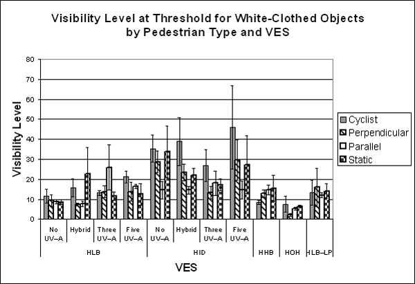 Figure 66. Bar graph. Threshold visibility level for white-clothed pedestrian objects.
A dosage factor was developed and calculated for the threshold values. This dosage factor evaluates the size of the object and the luminance from the object area, and it is defined as the product of the object luminance and the object size in steradians. According to Gibbons, Andersen, and Hankey, the dosage factor has shown some value in accounting for the object size at the threshold point.(4) The dosage factor for the black-clothed objects is shown in figure 67 and for the white-clothed objects in figure 68. The first item to note is that the range of values for both the black-clothed and the white-clothed objects is the same; however, there is not a single value that is evident as the required threshold. There seem to be differences between the threshold levels by VES, particularly for the white-clothed static pedestrian; however, the comparison of the HLB-based VESs to the HHB, HOH, and HLB–LP VESs shows a generally consistent threshold value. 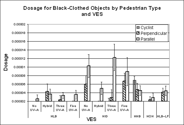 Figure 67. Bar graph. Threshold dosage factor for black-clothed pedestrian objects.
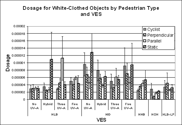 Figure 68. Bar graph. Threshold dosage factor for white-clothed pedestrian objects.
In the assessment of the threshold requirements for the detection and recognition of the objects, the metrics of the Weber contrast ratio and VL as well as a dosage factor seem to provide some insight, but they do not provide a single threshold value for all of the objects and VESs. The Weber ratio provides some equivalent results, and it is the most closely correlated to the visibility distance results, but it does not account for the object size. The VL provides some insight into what attracts the eye of the participant, but it is not comparable between white-clothed and dark-clothed pedestrians. The dosage factor provides both an equivalent basis for comparison between objects and some comparable results, but it has evident differences as well. One of the issues not considered in this analysis is that of movement. During the ENV visual performance studies, the cyclist and perpendicular and parallel pedestrians were all in motion, either walking or riding a bicycle. The cyclist and the perpendicular pedestrian moved across the roadway, and the parallel pedestrian moved along the shoulder. The sensitivity of the eye to motion and the direction of the motion may have influenced the object visibility. Similarly, the changes of the background as the object moved and the changes in the contrast with motion both would have influenced the visibility. This motion is a factor not accounted for in any of the metrics, and it may explain some of the evident differences.
|

