
The purpose of this technical document is to describe the modeling process and analysis used to support the Federal Highway Administration (FHWA) carbon monoxide (CO) categorical hot-spot finding for intersections using MOVES2014a as described in later sections of this document. The modeling does not apply to California which uses EMFAC for its emissions model. The modeling process described in this document includes the input determination process, use of guidance materials, MOVES2014a emission modeling, and CAL3QHC dispersion modeling. This document only covers the modeling process that was used to support FHWA’s CO categorical hot-spot finding and is not intended to describe the implementation of results. FHWA’s CO categorical hot-spot memorandum and finding are available on FHWA’s CO categorical hot-spot finding website. Modeling files for MOVES2014a and CAL3QHC are available via request from FHWA’s Air Quality and Transportation Conformity Team at TAQC@dot.gov.
A CO categorical hot-spot finding provision was added in the January 24, 2008 final conformity rule at 40 CFR 93.123(a)(3) and explained in the preamble at 73 FR 4432-4434. This provision allows the U.S. Department of Transportation (USDOT), in consultation with the Environmental Protection Agency (EPA) to make a categorical hot-spot finding that the requirements in 40 CFR 93.116(a) are met without any further hot-spot analysis for applicable FHWA and FTA projects in CO nonattainment or maintenance areas. This finding must be based on “appropriate modeling[*]” and may consider current air quality circumstances for a given CO nonattainment or maintenance area.[†]
In order to meet the requirements in 40 CFR 93.123(a)(3), FHWA, in consultation with the EPA, conducted a screening analysis of a large intersection operating at capacity using MOVES2014a and CAL3QHC to demonstrate that projects meeting the finding’s parameters would not produce a CO concentration higher than what was modeled and, when combined with background concentrations, would not violate the National Ambient Air Quality Standard (NAAQS) for CO. The analysis conducted here met all the conformity requirements for a CO hot-spot analysis including 40 CFR 93.110, 93.111, 93.116(a), and 93.123(a) and (c) by using the latest versions of appropriate models; MOVES2014a1 and CAL3QHC2; and consistent with EPA’s guidance: “Guideline for Modeling Carbon Monoxide from Roadway Intersections”3 (1992 CO Guideline) and “Using MOVES2014 in Project Level Carbon Monoxide Analyses”5 (2015 CO MOVES2014 Guidance). In accordance with the Highway Capacity Manual4 (HCM2010), we relied on the HCM2010 Software to develop our traffic volumes and speeds (HCM2010, pg. 18-31). As noted in section 1.1 above, the MOVES-based analysis conducted here cannot be used in California.
Figure 1 presents an overview of the modeling process. Reference to sections where the description of work occurs is included in the figure.
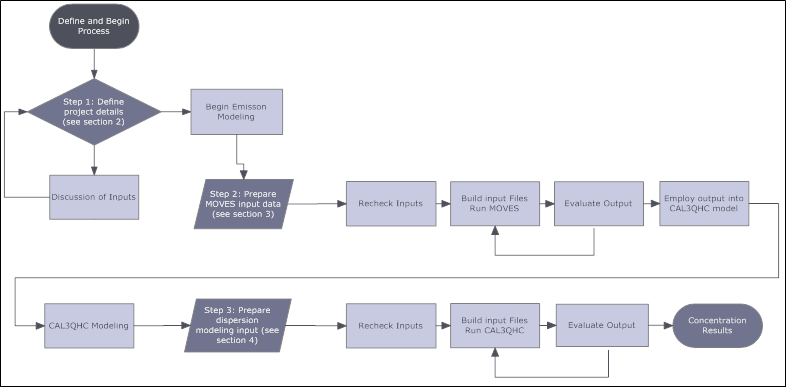
Figure 1. Modeling Process Overview
Define and Begin Process
Goes to: Step 1: Define project details (see section 2)
Goes to either:
Discussion of Inputs
Goes back to Step 1: Define project details (see section 2)
Begin Emissions Modeling
Goes to Step 2: Prepare MOVES input data (see section 3)
Goes to Recheck Inputs
Goes to Build input Files and Run MOVES
Goes to Evaluate Output
Goes to either:
Employ output into CAL3QHC model
Goes to CAL3QHC Modeling
Goes to Step 3: Prepare dispersion modeling input (see section 4)
Goes to Recheck Inputs
Goes to Build input Files and Run CAL3QHC
Goes to Evaluate Output
Goes to either:
The goal of the analysis was to model a large intersection using MOVES2014a and CAL3QHC operating at capacity so that projects meeting the finding’s parameters would not produce a CO concentration higher than what was modeled and, when combined with background concentrations, would not violate the NAAQS for CO. It is important to note that background concentration would be a function of the particular project and will be provided by a project sponsor following the 1992 CO Guideline3. Section 2.2 provides a summary of the intersection project that was analyzed for the categorical hot-spot finding.
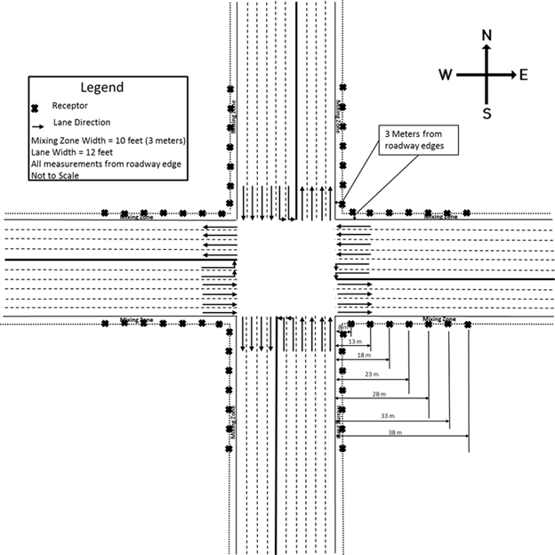
A large urban, signalized intersection was analyzed. The symmetrical intersection was modeled with each of the approaches and departures at 90 degree angles. The intersection included four approach lanes in each direction, four departure lanes in each direction, and two left turn lanes for each approach. The right lane in each direction was assumed to include both through and right turn movements. Lanes were assumed to be 12 feet wide in all cases. The intersection geometry modeled is shown graphically in Figure 2.
Using the Highway Capacity Software, the HCM20104 provides a methodology to calculate the approach volumes for a signalized intersection for Level of Service (LOS) E (defined as an average control delay greater than 80 seconds per vehicle). It was assumed that all approaches would have equal demand to represent a maximum total intersection throughput.
The assumptions made regarding the operation of the intersection of LOS E included allowing for a separate through and left-turn phases for each roadway for the total cycle length, and “green time” was allocated proportionately for each selected movement based on the demand. Given these assumptions and the roadway geometry shown in Figure 2, the Highway Capacity Software calculated a design flow rate of 2640 vehicles per hour for each approach leg. Of that total, 396 vehicles were assigned to the left-turn lanes and the remaining 2244 vehicles were assigned to the through lanes, including the shared through-right turn lane to characterize vehicle queuing at the intersection.
Directly related to the volume of an intersection is the signal timing. Based on the HCM20104, signal times were determined to be 130 seconds for the total cycle (red to red for one direction), an average green time of 41 seconds for the through and right turn movements occurring at the same time for opposing approaches, and 14 seconds for the average left turn movement concurrent in opposing directions.
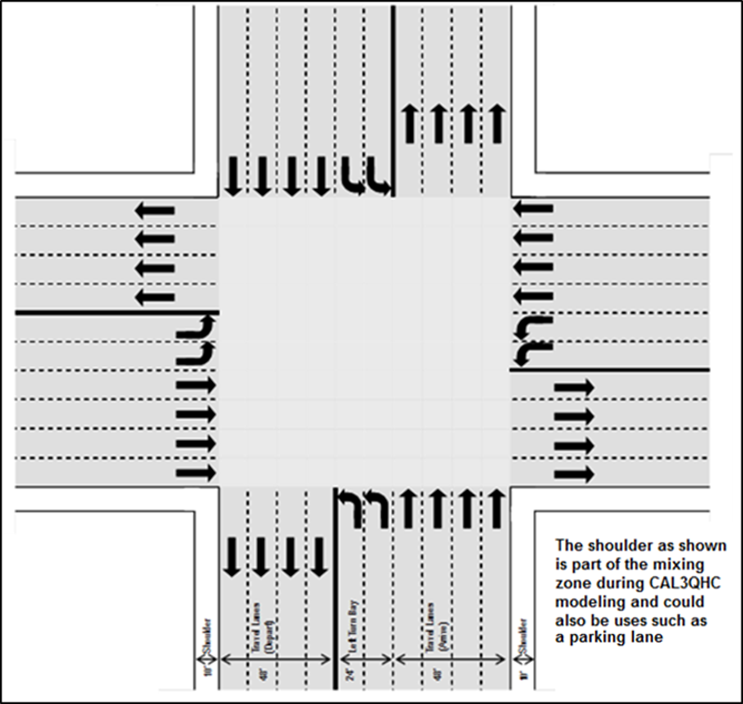
Figure 2.Geometry of Intersection Analyzed
The average approach and departure speeds were established as recommended in the1992 CO Guideline3. The speed was selected as 25 miles-per-hour per Table 4.2 in the 1992 CO Guideline3. While a range of 25 to 30 mph was given in Table 4.2, using 25 mph results in a greater emission rate when using MOVES2014a. Idle emission rates were also determined using MOVES2014a and more detail is included in Section 3. Queue lengths were determined internally by the CAL3QHC model during the modeling process which will be discussed in Section 4.
Because severe grades may pose a safety hazard and are not generally expected for intersections of this size, a more typical grade condition was selected. In this configuration, one approach and corresponding departure were assumed to be on an uphill grade of 2% while the parallel approach and departure were assumed to be on a downhill grade of 2%. The perpendicular approaches and departures were modeled with no grade (0%). Table 1 lists the final geometric and traffic parameters used in the modeling.
The MOVES2014a1 model was used for this analysis. Each MOVES input is discussed in the following sections and is consistent with 2015 CO MOVES2014 Guidance5. The MOVES2014a files and databases used in this analysis are available via request from FHWA’s Air Quality and Transportation Conformity Team at TAQC@dot.gov.
Description
The MOVES2014a inputs described in the RunSpec and Project Data Manager sections were used to model the Intersection scenario.
Scale
The CO hot-spot analysis is a project-level analysis using the project domain and Inventory calculation type. The inventory calculation was selected because it provides the information needed, when post processed (via EPA’s scripts), to get the emission rates needed for CAL3QHC.
Time Spans
2017 was chosen for the year of analysis because CO emission rates decline steadily in future years and 2017 represents the year in which the highest CO emission rates will occur and the first year this categorical finding will be used. Any year after 2017 would yield lower CO emission rates.
Following the 1992 CO Guideline3 and the 2015 CO MOVES2014 Guidance5, the month of January was selected. Refer to the Meteorology discussion within the Project Data Manager sub-section for more details.
MOVES requires either a weekday or weekend to be chosen for project-level modeling. Since either choice would not impact modeling results, the analysis was conducted for a weekday.
MOVES requires a specific hour to be chosen for project-level modeling; since only one hour is being modeled for this analysis and all project data is being provided for that hour, 8:00- 8:59 am was selected to represent peak hour data for the intersection.
Geographic Bounds
A custom domain was chosen utilizing national defaults for Barometric Pressure, Vapor Adjustment, Spill Adjustment, and the Geographic Phase-In Area (GPA) fraction parameters and is listed in Table 2. Vapor and Spill Adjustment parameters are not applicable to the Running Exhaust and Crankcase Running Exhaust processes and therefore not included in the analysis.
Generic County Parameters |
|
|---|---|
StateID |
99 |
CountyID |
1 |
GPA Fraction |
0 |
Barometric Pressure |
28.94 |
Vapor Adjustment |
0 |
Spill Adjustment |
0 |
Vehicles/Equipment
Since all MOVES vehicle types were assumed to be operating in the project area, in accordance with the 2015 CO MOVES2014 Guidance5 all 13 MOVES source use types were selected for the analysis. Table 3 lists the vehicle and fuel type combinations utilized in this analysis.
Source Use Types |
Fuel Type(s) |
|---|---|
Motorcycle |
Gasoline |
Passenger Car |
Diesel Fuel, Gasoline, Electricity, and Ethanol[‡] |
Passenger Truck |
Diesel Fuel, Gasoline, Electricity, and Ethanol |
Light Commercial Truck |
Diesel Fuel, Gasoline, Electricity, and Ethanol |
Refuse Truck |
Diesel Fuel and Gasoline |
Motor Home |
Diesel Fuel and Gasoline |
School Bus |
Diesel Fuel and Gasoline |
Transit Bus |
Diesel Fuel, Gasoline, and CNG |
Intercity Bus |
Diesel Fuel |
Single Unit Short-haul Truck |
Diesel Fuel and Gasoline |
Single Unit Long-haul Truck |
Diesel Fuel and Gasoline |
Combination Short-haul Truck |
Diesel Fuel and Gasoline |
Combination Long-haul Truck |
Diesel Fuel |
Road Type
The Urban Unrestricted Access road type was used to represent all Intersection links.
Pollutants and Processes
The intersection scenario required the Running Exhaust and Crankcase Running Exhaust emissions processes for CO to be selected.
Manage Input Data Sets
This panel was not used in this analysis, consistent with the EPA guidance, “Using MOVES2014 in Project-Level Carbon Monoxide Analyses.”[§]
Strategies
The Strategies Navigation Panel item is not applicable to this categorical finding.
Output
The output database utilized is available by request from FHWA’s Air Quality and Transportation Conformity Team at TAQC@dot.gov. Table 4 lists the General Output selections and Table 5 lists the Output emissions detail selections used for this analysis.
Heading |
Selection(s) |
|---|---|
Units |
Mass Units = Grams |
Energy Units = Million Btu |
|
Distance Units = Miles |
|
Activity |
Distance Traveled |
Source Hours Operating |
|
Population |
Advanced Performance Features
No Advanced Performance Features were utilized for the analysis.
Meteorology Data
Following the 1992 CO Guideline3 and the 2015 CO MOVES2014 Guidance5, and since this analysis is intended to apply to all the CO maintenance areas (except in CA), the analysis utilized an average January temperature of -10° Fahrenheit in order to permit wide applicability of the finding. “Relative humidity” was set at 100%. These values result in higher CO emission rates than an area with a higher average January temperature and a lower relative humidity. However, it is important to note that CO emission rates for diesel or gasoline vehicle types are not sensitive to temperature and relative humidity when temperature values are below 60° F for the relevant Running Exhaust and Crankcase Running Exhaust processes6.
Age Distribution
The 2015 CO MOVES2014 Guidance5 allows for default age distribution from MOVES to be used when no other state or local data is available. Because this analysis is not focused on a specific area, the national default age distribution representing the 2017 analysis year was used.
Fuel
The 2015 CO MOVES2014 Guidance5 recommends that the default MOVES fuel supply and fuel formulation data be utilized representing the project specific area. However, for the CO categorical hot-spot finding analysis, a fuel type with specific parameters that would yield the highest CO emission rates for 2017 was used, to have widest applicability.
In order to determine which gasoline fuel formulation would produce the highest CO emission rates, in a separate analysis, all 78 unique fuel formulations that appear in the MOVES2014a default database for the year 2017 were modeled, and the resulting CO emission rates compared. Fuel Formulation ID 3505 was determined to produce the highest CO emission rates compared to the other 77 gasoline fuel formulations available for the year 2017. Therefore, fuel formulation ID 3505 is utilized for this analysis for gasoline vehicles. Fuel Formulation ID 25005 is used for modeling diesel vehicles and is the default diesel fuel formulation for 2017. Fuel Formulation ID 30 was used to model CNG transit buses and is the 2017 default fuel formulation for CNG vehicles.
Fuel formulation parameters can significantly affect the CO emission rates.
Gasoline Fuel parameters that can affect CO emission rates include Reid Vapor Pressure (RVP), Sulfur Content, Ethanol (ETOH), and E200/E300 (percent of fuel evaporated at 200° and 300° Fahrenheit). Table 6 lists the fuel formulations used for this analysis.
The Fuel Usage Fraction was introduced with MOVES2014 and allows the user to apply an adjustment for E-85 usage among gasoline vehicles that are E-85 capable. Due to the CO emission rates for source types that utilize E-85 being lower compared to the CO emission rates of those source type that utilize gasoline, analysis assumes no E-85 utilization for E-85 capable vehicles. This will result in higher CO emission rates than if E-85 was included in the analysis.
The default for 2017 AVFT was utilized for this analysis.
Inspection and Maintenance (I/M) Programs
No I/M program was modeled in the analysis due to the variation in I/M programs across the CO maintenance areas. Also, including an I/M program would yield lower CO emission rates.
Link Source Types
A National Scale MOVES2014a run for 2017, which uses all MOVES defaults for that year, was the starting point for the Link Source Type input. Utilizing the vehicle miles traveled (VMT) information from the ‘movesactivityoutput’ table within the output database, the Source Type Distributions for Urban Unrestricted Road Type was obtained and transformed into a Source Type Hour Fraction for the intersection scenario. The Source Type Hour Fraction based upon the National Scale run was adjusted as described below to reflect a higher proportion of vehicles that have higher CO emission rates:
Table 7 lists the Link Source Type utilized for the intersection scenario.
Links
The intersection scenario was modeled using the Urban Unrestricted Access Road Type, as noted under Road Type above, with an average free flow speed of 25 mph at grades of +2%, -2%, and 0% (see Section 2.2 for discussion of grade). Idle conditions were also modeled for the intersection scenario.
CO emission rates in grams per vehicle mile (grams/veh-mile) were obtained for each link with exception of the idle link where CO emission rates are in grams-per–vehicle-hour (grams/veh-hour). In the emissions modeling, each link length was set to a 1 mile segment with a volume of 1000 vehicles per hour to allow ease in extracting the appropriate data, since emission rates rather than total emissions are needed. This link length and link volume is different from the link length and volume used in dispersion modeling described later in this report. Table 8 lists the characteristics and definitions associated with each link used in the MOVES portion of the analysis.
Link Drive Schedule
User-defined Link Drive Schedules were not utilized for this analysis.
Operating Mode Distribution
User-defined Operating Mode Distributions were not utilized for this analysis.
Off-Network
Off-Network links were not included in this analysis.
The analysis utilized the Inventory approach in obtaining MOVES2014a output consistent with the 2015 CO MOVES2014 Guidance 5. The CO emission rates for each link were obtained by executing the EPA provided CO_CAL3QHC_EF.sql script in MOVES2014a, which produced CO emission rates in grams per vehicle-mile. LinkID 500 represented a queue link at idle condition and the CO emission rate in grams per vehicle-hour was calculated by dividing the total emissions of the link by the 1000 vehicles assigned to the link over the hour modeled. Table 9 lists the emissions rates for the links associated with the intersection scenario and used with CAL3QHC for air quality dispersion modeling.
Dispersion modeling was completed using the CAL3QHC model, Version 2.02 and as described for CO screening analyses of highway-only projects by the 1992 CO Guideline3. The CAL3QHC files used in this analysis are available via request from FHWA’s Air Quality and Transportation Conformity Team at TAQC@dot.gov. The following discussion describes the inputs specific for CAL3QHC used in this analysis.
Dispersion Links
Dispersion links were extended out to 3000 feet from the intersection so that midblock receptor locations at 1500 feet from the intersection could be evaluated without end effects occurring. Figure 2 previously presented the geometry in the immediate vicinity of the intersection.
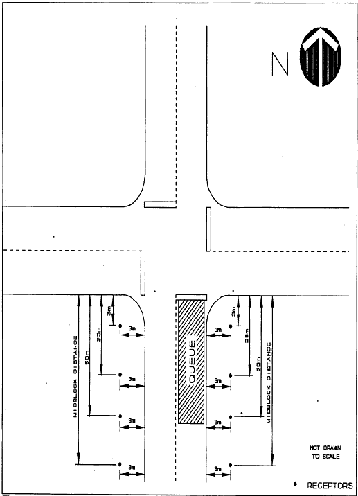
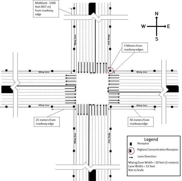
Receptors
Receptors were located according to the 1992 CO Guideline3 at no closer than 10 feet (3 meters) to the roadway edge to account for the mixing zone and extending away from the intersection out to midblock. The example receptor locations as described in the 1992 CO Guideline are shown in Figure 33. Receptors extending away from the intersection up to midblock conditions were used for this analysis. Figure 4 displays the receptor locations used for this 2017 CO Categorical Finding, consistent with the 1992 Guideline. In accordance with 40 CFR 93.123(a)(3), FHWA consulted with EPA in the development of this Finding. EPA requested additional receptors be analyzed at 5 m intervals. These additional receptors are presented in Figure 5.
Traffic Volume
The approach volume of 2640 vehicles per hour during the peak hour was used for this analysis as previously discussed in Section 2.2.
Vehicle Movements at Intersection
As mentioned in Section 2.2, movements were assumed to be 15% for left turns and 5% for right turns. This results in a high fraction of left turns and considerable idle time. Additionally, right turns were assumed to come to a complete stop and not proceed until a green signal phase occurred.
The total cycle length used was 130 seconds and developed based on traffic principles. Again, based on traffic principles, an average green time of 14 seconds was allocated for left turns and 41 seconds of green time for the right and through traffic. The lost time at the intersection was assumed to be 2 seconds per phase. This resulted in an average intersection delay of 78.5 seconds per vehicle, which corresponds to LOS E conditions approaching LOS F (which is defined as delay greater than 80 seconds per vehicle). Accordingly, the modeled intersection is theoretically functioning just before breakdown into a LOS F condition and represents the greatest delay of a functioning intersection.
Approach/Departure Speeds
Based on the 1992 CO Guideline3, a signalized approach/departure speed of 25 mph for urban conditions was used as described in Section 2.2. The appropriate emission factor was used as previously described in Section 3.
Meteorology
Wind. The worst case surface meteorology as prescribed in the 1992 CO Guidelines3 was used. Wind speed was assumed to be 1.0 meters-per-second resulting in the greatest predicted level when using the CAL3QHC model. The wind direction was again evaluated every 10 degrees from 0 to 360 degrees to insure the maximum concentration was predicted for the array of receptors accounting for the full range of possible wind directions.
Stability and Mixing Height. An urban worst case stability class of D and a mixing height of 1000 meters were utilized, consistent with the 1992 CO Guideline3.
Surface Characteristics
A surface roughness of 108 centimeters, corresponding to a single family residential condition, was used. This is based on the 1992 CO Guideline3 and the paper by Auer7 that explains that the use of the smallest value of surface roughness in an urban area allows prediction of greater CO concentrations.
CAL3QHC Output
A 1-hour averaging time was used. This resulted in 1-hour concentrations at the selected receptor locations being predicted. 8-hour concentrations were predicted using the EPA recommended persistence factor of 0.7, described in detail below in Section 6, Persistence Factor.
Summary of CAL3QHC Inputs
Table 10 summarizes the final input parameters used for modeling the intersection.
No background concentration values were included in the modeling since this will be a function of the project location and will be determined on a project-specific basis using the appropriate methodology such as described in the 1992 CO Guideline3.
The CO NAAQS consists of both 1-hour and 8-hour standards. To allow comparison to both the 1-hour and the 8-hour NAAQS for CO, the 1992 CO Guideline3 recommends using a persistence factor to convert peak 1-hour predicted concentrations to peak 8-hour estimations. Use of this persistence factor allows for the changes in traffic volumes and meteorological conditions over the 8-hour period as compared to the 1-hour period. If a local persistence factor based on monitoring data is unavailable, the 1992 CO Guideline3 recommends using a default persistence factor of 0.7.
For the intersection analysis the 1-hour concentration was first predicted using CAL3QHC. Then, using the procedure described above, the predicted 1-hour concentration was multiplied by the default persistence factor of 0.7 to allow estimation of the 8-hour concentration.
As presented in Section 3, the emission factors for the urban intersection were 5.581 grams-per-vehicle-mile for the 25 mph increasing grade (2%) and 3.401 grams-per-vehicle-mile for the down-grade (-2%). The emission factor for the level roadway was 4.304 grams-per-vehicle mile. The idle emission factor was 18.58 grams-per-hour. This resulted in a maximum predicted concentration of 2.4 parts-per-million for the 1-hour concentration (located at northeast corner receptor as shown in Figure 4) and using the 0.7 persistence factor, 1.7 parts-per-million for the 8-hour concentration. These values can be compared to the NAAQS of 35 ppm and 9 ppm for the 1-hour and 8-hour standards, respectively. Table 11 includes a summary of the key results of the analysis. As discussed in Section 4.1, additional receptors were modeled at the request of US EPA. None of the additional receptors in this informational analysis had higher concentrations than the highest receptor nearest the intersection and therefore did not change the results of the CO Categorical Finding.
Facility Type |
1-Hour Predicted Concentration (ppm) |
8-Hour Predicted Concentration (ppm) |
|---|---|---|
Intersection |
2.4* |
1.7 |
* Receptor location noted on Figure 4.
This document summarizes the technical information and methodology used to support FHWA’s categorical hot-spot finding for CO. Emission and dispersion modeling using MOVES2014a1 and CAL3QHC Version 2.02, respectively, are described in detail and the key results presented. Only urban cases were analyzed, since CO maintenance areas mainly cover these areas. A large intersection (4 through/right turn approaches and 2 left turn lanes) was evaluated. The predicted emission factors were used as input for dispersion modeling to determine the 1-hour predicted concentrations. The 8-hour concentrations were determined using the 1-hour predictions and the use of a 0.7 persistence factor. The analysis was intentionally performed in a way to allow results to reflect predicted concentrations greater than expected for most projects.
1 U.S. Environmental Protection Agency, MOVES2014a User Guide, EPA-420-15-095, Office of Transportation and Air Quality, November, 2015.
2 U.S. Environmental Protection Agency, CAL3QHC, Version 2.0 with a date of 04244, Technology Transfer Network, Support Center for Regulatory Atmospheric Modeling.
3 U.S. Environmental Protection Agency, Guideline for Modeling Carbon Monoxide from Roadway Intersections, EPA-454/R-92-005, Office of Air Quality Planning and Standards, November, 1992.
4 Highway Capacity Manual, Transportation Research Board, Washington, D.C., 2010.
5 U.S. Environmental Protection Agency, Using MOVES2014 in Project-Level Carbon Monoxide Analyses, EPA-420-B-15-028, Transportation and Regional Programs Division, Office of Transportation and Air Quality, March, 2015.
6 Choi, D., M. Beardsley, D. Brzezinski, J. Koupal, and J. Warila, MOVES Sensitivity Analysis: The Impacts of Temperature and Humidity on Emissions, U.S. Environmental Protection Agency, OTAQ, Ann Arbor, MI, no date specified.
7 Auer, A.H., Jr., "Correlation of Land Use and Cover with Meteorological Anomalies", Journal of Applied Meteorology, 1978.
[*] (40 CFR 123(a)(3)).
[†] EPA’s “Greenbook” states that, “As of September 27, 2010, all carbon monoxide areas have been redesignated to maintenance areas”
[‡] Ethanol Vehicles were selected on the ‘On Road Vehicle Equipment’ Navigation Panel, since vehicles that can run on E-85 (flex-fuel vehicles) are present in every state’s fleet. However, ethanol was not modeled in the analysis. In other words, all flex-fuel vehicles are using conventional gasoline in this analysis. This is explained further ‘Project Data Manager’ ‘Fuel Usage Fraction’ section.
[§] U.S. Environmental Protection Agency, “Using MOVES2014 in Project-Level Carbon Monoxide Analyses,” EPA420-B-15-028, March 2015.

