
Also available as Adobe PDF (2.4MB)
Cost Effectiveness Tables Rollout Webinar
FOREWORD
This CMAQ Cost-Effectiveness Tables Update is intended to provide information to assist States, MPOs and other project sponsors as they make the most efficient use of their CMAQ funding to reduce vehicle emissions and traffic congestion.
This document provides information regarding the development of estimates of cost-effectiveness for a range of representative project types previously funded under the CMAQ Program. Conclusions drawn from this analysis are confined to the CMAQ Program. Topics include: the analysis process and methodology, including the use of the MOtor Vehicle Emissions Simulator (MOVES) in determining emissions rates; key limitations of the analysis process; and the selection of specific project types for analysis. The results are displayed graphically by pollutant type in increasing order of median project cost. An aggregate table of summary finding displays results for all pollutants and all project types.
The 2020 CMAQ Cost-Effectiveness Tables Update compares the cost-effectiveness of projects funded by the Congestion Mitigation and Air Quality Improvement (CMAQ) Program, in accordance with 23 U.S.C. 149(i)(2). State and local governments can use CMAQ funding to support projects and programs that will reduce emissions in areas that are in non-attainment or maintenance of the National Ambient Air Quality Standards (NAAQs) for three criteria pollutants: ozone, carbon monoxide (CO), and particulate matter (PM10 and PM2.5). The cost-effectiveness analysis also considers applicable precursors, namely nitrogen oxides (NOx) and volatile organic compounds (VOCs). Note that conclusions drawn from this 2020 Cost-Effectiveness Tables analysis are only applicable to the CMAQ Program.
This report updates the first set of tables completed in 2015. This version includes a revision to the project types list to reflect information from the CMAQ Public Access System (PAS), and updated emissions modeling using the U.S. Environmental Protection Agency's MOtor Vehicle Emissions Simulator (MOVES) software.
A series of tables present the cost-effectiveness, in dollars per ton of emissions reduced, of eligible CMAQ project types. The 2020 Cost-Effectiveness Tables Update includes analysis of 21 project types, which are generally consistent with the 2015 study. New project types in this study are marked with an asterisk below. This study added several categories and refined others (e.g., bicycle and pedestrian improvements). Projects types in the 2020 Update include:
Findings are presented in terms of median cost-effectiveness by project type and individual pollutant. Project types were rated as having strong, weak, or mixed cost-effectiveness by summing the median cost-effectiveness across all pollutants. Strong cost-effectiveness is characterized as costing less than $2.8M per ton of emissions reduced across all pollutants, mixed cost-effectiveness as costing between $2.8M and $8.8M per ton, and weak cost-effectiveness as costing $8.8M or more per ton.
Project types which demonstrate strong cost-effectiveness for PM10 and PM2.5 include dust mitigation and idle reduction technologies. For example, dust mitigation projects can reduce PM pollution for less than $15,000 per ton. Electric vehicle charging stations, carsharing, transit service expansions, natural gas refueling facilities, and park and ride programs show strong cost-effectiveness for reducing CO emissions – the first three project types are also especially strong for NOx and VOCs. Most projects with strong cost-effectiveness tend to target a particular pollutant (e.g., dust mitigation) or significantly reduce vehicle miles traveled (VMT) (e.g., transit service expansions).
Projects showing the weakest cost-effectiveness include heavy-duty vehicle replacements, bikesharing, intersection improvements, and subsidized transit fare programs. In the case of heavy-duty vehicle replacements and intersection improvements, both project types change the profiles of existing emissions, but neither removes vehicle activity entirely. Heavy-duty vehicle replacements show especially low cost-effectiveness for VOCs and PM, as these vehicles emit large amounts of these pollutants regardless of fuel type. In some cases, emissions from replacement vehicles can be significantly higher for specific pollutants. For example, replacing a diesel bus with a compressed natural gas (CNG) bus will increase PM emissions despite lowering all other criteria pollutants.1Some project types that demonstrate weak cost-effectiveness, such as bikesharing and bicycle and pedestrian improvements, significantly reduce vehicle activity but have high start-up costs.
Along with the analysis of emission impacts, the 2020 Cost-Effectiveness Tables Update also includes an analysis of congestion impacts, measured as reductions in vehicle-hours at idle (e.g., time queuing to pass through an intersection). Three of the project types analyzed may reduce congestion, measured on the basis of travel time per hour saved: intersection improvements (e.g., left turn lanes, signalization), roundabouts, and incident management.
It is important to acknowledge that cost-effectiveness with respect to reducing pollutant emissions and congestion is not necessarily the only reason to implement a given project. Different projects can provide a wide range of benefits (e.g., reductions in fuel consumption, safety improvements) that might make them worth pursuing. For example, a new bicycle lane may bring safety benefits, in addition to air quality improvements. Cost-effectiveness should be considered alongside these other benefits when determining project priorities, noting however that CMAQ-funded projects must demonstrate emissions benefits.
This document estimates and compares the cost-effectiveness of representative projects eligible for the Congestion Mitigation and Air Quality Improvement (CMAQ) Program as required under 23 U.S.C. 149(i)(2). 23 U.S.C. 149(b) and the 2013 CMAQ Interim Guidance detail project eligibility for the CMAQ program.2
The 2020 Cost-Effectiveness Tables Update is organized into four parts. The first section summarizes the findings of the cost-effectiveness study. The second section describes the CMAQ program and the cost-effectiveness evaluation requirement, and summarizes related research under prior legislation. The third section describes the research objective, the CMAQ project types analyzed, and the analytical scenario methods used to calculate cost-effectiveness for each project type. This section also includes data sources and assumptions used for modeling emissions impacts for each of the evaluated project types. The final section presents the cost-effectiveness estimates by project type.
This section presents summary findings from the 2020 Cost-Effectiveness Tables Update. Table 1 compares the median cost-effectiveness estimates for each project type and pollutant in the analysis, measured in dollars per ton of pollutant reduced. The shading in the table indicates the relative performance of the various project types – lighter shades indicate stronger cost-effectiveness. Blank cells indicate that the project type has negligible impact on a particular pollutant. Project types are ranked from most to least cost-effective based on overall cost-effectiveness across all criteria pollutants (i.e., "Total Cost per Ton" in Table 1). Note, however, that projects are typically chosen for their effectiveness at reducing certain pollutants, rather than their across-the-board effects. The subsequent sections on individual pollutants provide additional context.
The suite of project types was ranked by first summing the median3 cost-effectiveness across all pollutants for each project type, and then ordering the list of project types from most to least cost-effective (dollars per ton of emissions reduced). This arrangement provides the overall cost-effectiveness of each project across all of the criteria pollutants, and this list was then divided into thirds: strong, mixed, and weak cost-effectiveness. Project types with overall strong cost-effectiveness are characterized as costing less than $2.8M per ton of emissions reduced, with overall mixed cost-effectiveness between $2.8M and $8.8M per ton, and with overall weak cost-effectiveness costing $8.8M or more per ton. The discussion of individual pollutants examines these categories more closely, indicating what distinguishes the strong, mixed, and weakly cost-effective projects from each other within each category.
| Project Type | CO | NOx | VOCs | PM10 | PM2.5 | Total Median Cost per Ton |
|---|---|---|---|---|---|---|
| Dust Mitigation | A | B | $15,932 | |||
| Idle Reduction Strategies | A | A | A | B | B | $58,999 |
| Diesel Engine Retrofit Technologies | B | B | C | D | D | $407,684 |
| Intermodal Freight Facilities and Programs | B | A | C | D | D | $494,834 |
| Carsharing | A | B | B | D | E | $766,199 |
| Incident Management | B | B | D | D | D | $1,071,991 |
| Transit Service Expansion | A | C | C | E | F | $2,766,431 |
| Traffic Signal Synchronization | C | D | F | D | F | $3,042,950 |
| Park and Ride | A | C | D | E | F | $3,622,288 |
| Natural Gas Re-Fueling Infrastructure | A | B | D | F | F | $3,675,107 |
| Electric Vehicle Charging Stations | A | C | D | F | F | $6,380,581 |
| Transit Amenity Improvements | B | D | D | F | G | $7,457,446 |
| Rideshare Programs | B | D | D | F | G | $8,194,085 |
| Roundabouts | D | D | F | G | F | $8,786,402 |
| Extreme Temperature Cold-start Technologies | B | F | D | F | F | $10,850,034 |
| Bikesharing | B | G | F | F | G | $13,834,816 |
| Bicycle and Pedestrian Improvement Projects | B | D | E | F | H | $19,423,016 |
| Intersection Improvements | D | F | F | H | H | $30,823,921 |
| Employee Transit Benefits | D | F | F | H | I | $50,281,268 |
| Subsidized Transit Fares | D | F | F | H | I | $50,281,268 |
| Heavy-Duty Vehicle Replacements | D | D | F | I | I | $69,830,233 |
| Median Cost-Effectiveness (Dollars per Ton Reduced) | |
|---|---|
| A | <10,000 |
| B | 10,000 - 50,000 |
| C | 50,000 - 100,000 |
| D | 100,000 - 500,000 |
| E | 500,000 - 1,000,000 |
| F | 1,000,000 - 5,000,000 |
| G | 5,000,000 - 10,000,000 |
| H | 10,000,000 - 20,000,000 |
| I | >20,000,000 |
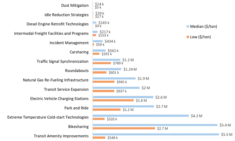
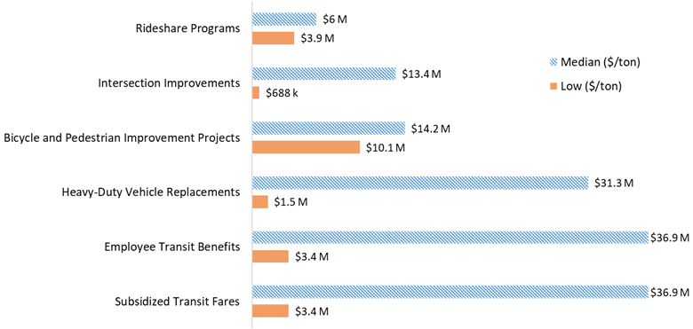
Please note that the charts in the following sections are split between higher and lower cost projects (two charts for each pollutant with different scales). The splitting is not the result of analysis, but purely for graphical purposes to aid nominal comparisons between projects.
Both median and low cost estimates ($/ton) are provided in the following figures; for many projects types, the lower-end estimates of cost-effectiveness are significantly lower than the median, indicating skewness in the cost data. The relevance of medians and skewness to the analysis are discussed in more detail in later sections (Assumptions and Limitations and Cost-Effectiveness by Project Type).
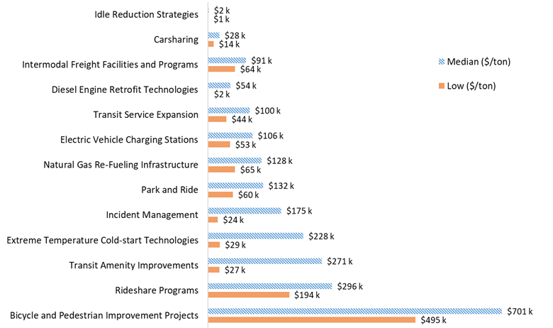
| CO | Median ($/ton) | Low ($/ton) |
|---|---|---|
| Dust Mitigation | ||
| Idle Reduction Strategies | 1,017 | 600.7 |
| Carsharing | 1,674 | 867.9 |
| Transit Service Expansion | 6,029 | 2642.8 |
| Electric Vehicle Charging Stations | 6,742 | 3371.1 |
| Park and Ride | 7,986 | 3637.3 |
| Natural Gas Re-Fueling Infrastructure | 9,413 | 4765.3 |
| Diesel Engine Retrofit Technologies | 14,671 | 452.0 |
| Bikesharing | 16,111 | 8055.5 |
| Transit Amenity Improvements | 16,441 | 1644.0 |
| Rideshare Programs | 17,901 | 11747.6 |
| Intermodal Freight Facilities and Programs | 23,677 | 16674.2 |
| Incident Management | 32,995 | 4495.6 |
| Extreme Temperature Cold-start Technologies | 35,410 | 4708.3 |
| Bicycle and Pedestrian Improvement Projects | 42,432 | 29952.1 |
| Traffic Signal Synchronization | 53,256 | 24547.5 |
| Employee Transit Benefits | 110,850 | 10275.4 |
| Subsidized Transit Fares | 110,850 | 10275.4 |
| Roundabouts | 195,881 | 53763.5 |
| Heavy-Duty Vehicle Replacements | 317,016 | 23165.2 |
| Intersection Improvements | 452,436 | 23003.5 |
Projects most effective at reducing CO reduce light-duty vehicle (LDV) activity or heavy-duty vehicle idling. The two most effective project types are diesel idle reduction strategies and carsharing. Median costs of these project types are around $1,000 to $1,500 per ton CO reduced; low-end estimates are around $600 to $850 per ton.
A large proportion of the other project types studied also exhibit strong cost-effectiveness for reducing CO emissions. Transit service expansions, electric vehicle charging stations, park and ride, natural gas refueling infrastructure, bikesharing, ridesharing, and transit amenity improvements all had median costs less than $21,000 per ton of CO reduced. Park and ride, transit service expansion, and bicycle and transit amenity improvements encourage mode shift, thus reducing VMT and emissions. Extreme-temperature cold start technologies reduce CO emissions during vehicle starts in cold climates. Incident management projects reduce engine idling in sudden congestion, reducing per-mile CO emissions.
Weaker strategies only marginally affect vehicular travel or are not directed at reducing CO. Heavy-duty vehicle diesel engine replacements address the inefficiencies of highly polluting older diesel vehicles, while intersection improvements smooth traffic operations to reduce idling, one of the more polluting phases of engine operation.
| NOx | Median ($/ton) | Low ($/ton) |
|---|---|---|
| Dust Mitigation | ||
| Idle Reduction Strategies | 421 | 248.8 |
| Intermodal Freight Facilities and Programs | 7,661 | 5394.9 |
| Carsharing | 19,020 | 9862.6 |
| Natural Gas Re-Fueling Infrastructure | 19,702 | 9974.0 |
| Diesel Engine Retrofit Technologies | 22,133 | 2685.0 |
| Incident Management | 31,708 | 4320.3 |
| Transit Service Expansion | 69,251 | 32509.2 |
| Electric Vehicle Charging Stations | 72,469 | 36234.4 |
| Park and Ride | 90,028 | 41005.9 |
| Transit Amenity Improvements | 185,347 | 18535.0 |
| Rideshare Programs | 203,417 | 133492.3 |
| Heavy-Duty Vehicle Replacements | 309,889 | 34018.4 |
| Traffic Signal Synchronization | 360,647 | 129377.0 |
| Roundabouts | 434,343 | 119534.4 |
| Bicycle and Pedestrian Improvement Projects | 482,173 | 340357.6 |
| Intersection Improvements | 1,003,227 | 51144.5 |
| Employee Transit Benefits | 1,249,687 | 115841.8 |
| Subsidized Transit Fares | 1,249,687 | 115841.8 |
| Extreme Temperature Cold-start Technologies | 1,700,985 | 382223.9 |
| Bikesharing | 5,409,021 | 91537.6 |
Projects that reduce engine idling show the strongest cost-effectiveness for reducing NOx. These projects include idle reduction strategies, carsharing, natural gas refueling infrastructure, and diesel engine retrofits; all of which either directly reduce diesel engine idling pollution (anti-idle strategies, natural gas, retrofits) or remove excess vehicles from the road (carsharing, intermodal freight). Incident management is also relatively cost-effective for reducing NOx. The median cost per ton of NOx reduced for these highly cost-effective projects generally is less than $30,000. Similarly, projects that generally reduce LDV activity and idling, including electric vehicle charging stations, transit service expansion, and park and ride, are also relatively effective at reducing NOx; median costs are between $30,000 and $90,000.
Transit amenity improvements, heavy-duty replacements, ridesharing, roundabouts, transit amenity improvements, and traffic signal synchronizations show mixed cost-effectiveness for reducing NOx emissions, with median costs between about $185,000 and $480,000 per ton reduced. These projects also all reduce engine idling or LDV activity. However, they tend to be weakened by only marginal effects on travel behavior, high capital costs, or both.
Less cost-effective projects have minimal effects on vehicle activity, such as intersection improvements, transit subsidies, and bicycle and pedestrian projects. Bikesharing and bicycle and pedestrian improvements can involve expensive start-up costs that weaken their cost-effectiveness.
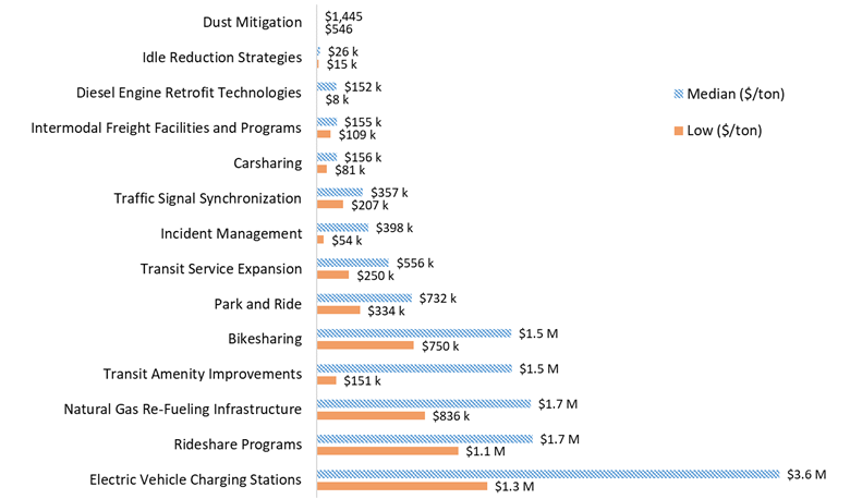
| VOCs | Median ($/ton) | Low ($/ton) |
|---|---|---|
| Dust Mitigation | ||
| Idle Reduction Strategies | 1,924 | 1136.3 |
| Carsharing | 27,650 | 14337.4 |
| Intermodal Freight Facilities and Programs | 91,297 | 64293.4 |
| Diesel Engine Retrofit Technologies | 53,831 | 1678.0 |
| Transit Service Expansion | 99,652 | 43865.4 |
| Electric Vehicle Charging Stations | 106,382 | 53191.0 |
| Natural Gas Re-Fueling Infrastructure | 128,388 | 64996.6 |
| Park and Ride | 131,848 | 60054.1 |
| Incident Management | 175,407 | 23899.7 |
| Extreme Temperature Cold-start Technologies | 227,961 | 28551.1 |
| Transit Amenity Improvements | 271,445 | 27144.0 |
| Rideshare Programs | 295,708 | 194058.6 |
| Bicycle and Pedestrian Improvement Projects | 700,938 | 494780.1 |
| Traffic Signal Synchronization | 1,067,924 | 543184.8 |
| Bikesharing | 1,500,331 | 133068.8 |
| Roundabouts | 1,611,762 | 448334.7 |
| Employee Transit Benefits | 1,830,196 | 169653.0 |
| Subsidized Transit Fares | 1,830,196 | 169653.0 |
| Intersection Improvements | 3,722,777 | 191826.3 |
| Heavy-Duty Vehicle Replacements | 3,909,224 | 180660.4 |
Similar to NOx, projects with strong cost-effectiveness for VOCs include projects that reduce engine idling and fuel consumption, in addition to other strategies targeting ozone reduction (i.e., engine retrofits). Intermodal freight facilities and programs are also highly cost-effective as they shift freight operations to more fuel-efficient modes such as rail and maritime transport. The median cost for these projects is between about $2,000 and $90,000 per ton of VOCs reduced.
As with other pollutants, park and ride and incident management projects that generally reduce traffic idling on the roadway are also very effective. Transit service expansion and electric vehicle charging stations, which facilitate mode shift and a reduction in overall VMT are similarly effective. The median cost for these projects is between $100,000 and $175,000 per ton of VOCs.
Less cost-effective projects (e.g., vehicle replacements) generally have marginal effects on fuel consumption. These include projects that result in marginal effects on vehicle activity (e.g., transit amenity improvements, traffic signal synchronization, intersection improvements, and roundabouts); as with NOx, bicycle and pedestrian projects are significantly less cost-effective due to large capital costs. These less cost-effective projects have a median cost greater than $200,000, with more extreme cases costing between $1 and nearly 4 million per ton of VOCs.
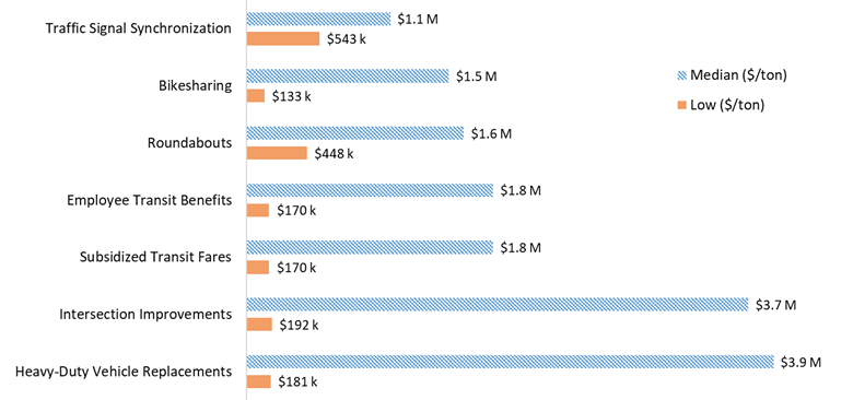
| PM10 | Median ($/ton) | Low ($/ton) |
|---|---|---|
| Dust Mitigation | 1,445 | 546.0 |
| Idle Reduction Strategies | 26,187 | 15461.8 |
| Diesel Engine Retrofit Technologies | 151,919 | 7961.0 |
| Intermodal Freight Facilities and Programs | 154,839 | 109041.4 |
| Carsharing | 155,879 | 80825.9 |
| Traffic Signal Synchronization | 356,543 | 206619.9 |
| Incident Management | 398,231 | 54260.2 |
| Transit Service Expansion | 556,301 | 249836.4 |
| Park and Ride | 732,201 | 333502.4 |
| Bikesharing | 1,500,331 | 750165.7 |
| Transit Amenity Improvements | 1,507,431 | 150743.0 |
| Natural Gas Re-Fueling Infrastructure | 1,651,129 | 835883.8 |
| Rideshare Programs | 1,667,035 | 1093991.7 |
| Electric Vehicle Charging Stations | 3,566,288 | 1314350.0 |
| Bicycle and Pedestrian Improvement Projects | 3,951,490 | 2789287.3 |
| Extreme Temperature Cold-start Technologies | 4,714,771 | 460251.5 |
| Roundabouts | 5,305,408 | 1472587.6 |
| Employee Transit Benefits | 10,163,738 | 942144.2 |
| Subsidized Transit Fares | 10,163,738 | 942144.2 |
| Intersection Improvements | 12,254,198 | 630067.4 |
| Heavy-Duty Vehicle Replacements | 33,962,799 | 1378699.8 |
Projects most cost-effective at reducing PM10 include those that mitigate fugitive dust. The median cost of these projects is $1,500 per ton of PM10. Other very cost-effective projects include those that either substantially reduce idling or allow for cleaner fuel combustion through retrofits or vehicle replacements, especially for diesel engines. Intermodal freight facilities and programs, carsharing, traffic signal synchronization, and incident management each cost less than $400,000 per ton of PM10 reduced.
The group showing the next strongest cost-effectiveness for reducing this category of emissions included transit service expansion, park and ride, roundabouts, bikesharing, natural gas refueling, and ridesharing. These projects all cost between about $500,000 and $1.7 million. Each of these projects only marginally impacts engine idling or other dust suppression activities, though they do have impact to some extent.
In general, less cost-effective projects (e.g., transit benefits) do not focus on reducing heavy-duty idling or other dust suppression activities. These include bikesharing, extreme-temperature cold-start technologies, and intersection improvements. The median cost of these projects ranges from $4 to in excess of $30 million.
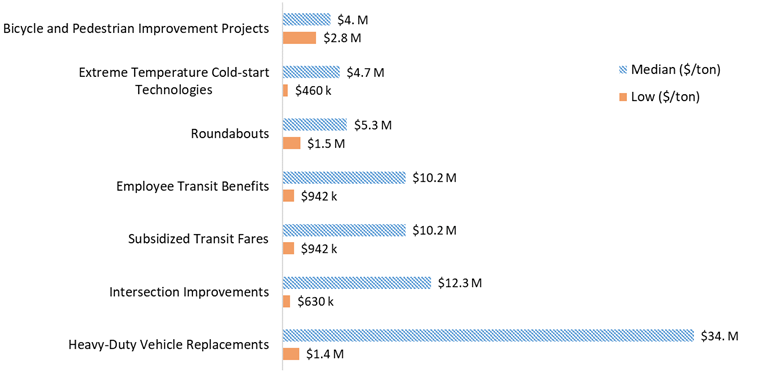
| PM2.5 | Median ($/ton) | Low ($/ton) |
|---|---|---|
| Dust Mitigation | 14,487 | 5478.0 |
| Idle Reduction Strategies | 29,450 | 17387.9 |
| Diesel Engine Retrofit Technologies | 165,130 | 8653.0 |
| Intermodal Freight Facilities and Programs | 217,360 | 153070.6 |
| Incident Management | 433,651 | 59086.2 |
| Carsharing | 561,976 | 291395.1 |
| Traffic Signal Synchronization | 1,204,581 | 788998.7 |
| Roundabouts | 1,239,008 | 601074.1 |
| Natural Gas Re-Fueling Infrastructure | 1,866,475 | 944903.0 |
| Transit Service Expansion | 2,035,198 | 937343.9 |
| Electric Vehicle Charging Stations | 2,628,700 | 1783143.9 |
| Park and Ride | 2,660,225 | 1211677.7 |
| Extreme Temperature Cold-start Technologies | 4,170,908 | 520273.1 |
| Bikesharing | 5,409,021 | 2704510.6 |
| Transit Amenity Improvements | 5,476,783 | 547678.0 |
| Rideshare Programs | 6,010,024 | 3944078.0 |
| Intersection Improvements | 13,391,283 | 688323.0 |
| Bicycle and Pedestrian Improvement Projects | 14,245,982 | 10055987.3 |
| Heavy-Duty Vehicle Replacements | 31,331,304 | 1498597.7 |
| Employee Transit Benefits | 36,926,797 | 3422989.6 |
| Subsidized Transit Fares | 36,926,797 | 3422989.6 |
As with PM10, projects most cost-effective at reducing PM2.5 include projects that mitigate fugitive dust and those that either reduce idling or involve retrofits strategies. Incident management, carsharing, and intermodal freight projects are also very effective at reducing PM emissions, with median cost of these projects being less than $600,000 per ton of PM2.5.
The next most cost-effective group of projects includes traffic signal synchronization, roundabouts, natural gas refueling, and transit service expansion, where the median cost of these projects ranges between $1.2 and $2 million.
As a rule, projects showing weaker cost-effectiveness do not focus on these activities (traffic flow improvements, transit service expansion, etc.). Programs such as bikesharing, transit amenity improvements, extreme-temperature cold-start technologies, intersection improvements, and transit fare subsidies can cost between $6 and $37 million per ton of PM2.5 reduced.
The analysis indicates that certain projects are particularly cost-effective for reducing the CMAQ pollutants and precursors across the board (overall cost-effectiveness):
| Project Type | Pollutants |
|---|---|
| Dust Mitigation | PM |
| Idle Reduction Strategies | All pollutants |
| Diesel Engine Retrofit Technologies | CO, NOx, VOCs |
| Intermodal Freight Facilities and Programs | CO, NOx, VOCs |
| Carsharing | CO, NOx, VOCs |
| Incident Management | CO, NOx |
| Transit Service Expansion | CO, NOx, VOCs |
In particular, dust mitigation reduces PM pollution for less than $15,000 per ton (CO, NOx, and VOCs emissions were not quantified for dust mitigation projects, which in practice have no effect on CO, NOx, or VOCs). Idle reduction strategies are also cost effective for reducing PM, while also contributing to substantial reductions in CO, NOx, and VOCs.
Diesel engine retrofits are particularly cost effective in reducing CO, NOx, and VOCs, and also lead to considerable reductions in PM. Car sharing and transit service expansions also strong cost-effectiveness across the board, as these projects reduce the number of light-duty vehicles on the road and may include use of alternative fuel transit vehicles.
Intermodal freight projects are especially cost-effective for reducing NOx and VOCs. These projects are generally cost-effective for reducing other pollutants as well, though the emphasis on heavy-duty freight increases the effect for NOx and VOCs.
Several project types demonstrated weak cost-effectiveness overall. These project types include:
| Project Type | Pollutants |
|---|---|
| Extreme Temperature Cold-start Technologies | NOx, PM |
| Bikesharing | NOx, VOCs, PM |
| Bicycle and Pedestrian Improvements | PM |
| Intersection Improvements | NOx, VOCs, PM |
| Subsidized Transit Fares/Employee Transit Benefits | NOx, VOCs, PM |
| Heavy-Duty Vehicle Replacements | VOCs, PM |
Two major themes apply to these projects. First, most are associated with large capital expenditures that dampen the overall effectiveness of the project, even where emissions savings are large. For example, bikesharing and bicycle/pedestrian infrastructure projects shift motorized trips to non-motorized trips, effectively reducing those substituted emissions to zero. However, the high start-up cost to construct the infrastructure obscures benefits in this analysis framework. This illustrates a limitation of using direct cost as the basis for evaluating investments such as CMAQ projects: it prioritizes "one-shot" approaches with large effects in a single investment, rather than more distributed effects that are difficult to attribute or that accumulate variably over time. This high capital cost theme is true of extreme-temperature cold-start programs for a similar reason, in that few places in the U.S. require such a deployment – they are primarily limited to the State of Alaska.
Second, most of the projects demonstrating weak cost-effectiveness do not affect existing activity, and thus have marginal effects on emissions. For example, a subsidized transit fare program may only encourage the marginal traveler who lives in an area with high transit accessibility to switch to transit. There is no overall change to the transit service provided, so the majority of the polluting activity and related travel behavior remain after the program is implemented. This is also true of intersection improvements, which make similarly marginal changes to travel speed or drive cycle, and of vehicle replacements: in the grand scheme, both have an effect on existing emissions, but neither are as effective as removing polluting vehicle trips from the road.
Heavy-duty vehicle replacements show extremely low cost-effectiveness for VOCs and PM. This can be attributed to the fact that heavy-duty vehicles emit large amounts of these pollutants, regardless of fuel type. In some cases, emission rates for replacement vehicles (e.g., replacing a diesel transit buses with a CNG bus) can be significantly higher for specific pollutants.5 Simply replacing the vehicle with a newer model year or different fuel type may change the emissions profile and cause some reductions, but is comparatively less effective because it does not reduce heavy-duty emitting activity.
The remaining project types demonstrated competitive cost-effectiveness for at least some pollutants in the analysis (Table 4). Despite strong cost-effectiveness for some categories (see Table 1), the higher costs per ton in other categories lowered the overall cost-effectiveness for the project type.
| Project Type | Strong Cost-Effectiveness | Mixed Cost-Effectiveness | Weak Cost-Effectiveness |
|---|---|---|---|
| Traffic Signal Synchronization | CO | NOx, VOCs, PM10, PM2.5 | - |
| Park and Ride | CO, NOx | VOCs, PM10 | PM2.5 |
| Natural Gas Re-Fueling Infrastructure | CO, NOx | VOCs, PM10, PM2.5 | - |
| Electric Vehicle Charging Stations | CO, NOx | VOCs, PM10, PM2.5 | - |
| Transit Amenity Improvements | CO | NOx, VOCs, PM10 | PM2.5 |
| Rideshare Programs | CO | NOx, VOCs, PM10 | PM2.5 |
| Roundabouts | - | CO, NOx, VOCs, PM2.5 | PM10 |
Several of these project types had strong cost-effectiveness for some pollutants. Electric vehicle charging stations are especially cost-effective for CO and NOx, but have comparatively weak cost-effectiveness at reducing PM emissions. Similarly, park and ride projects and natural gas refueling facility projects both have strong cost-effectiveness in reducing CO and NOx emissions, but display weak cost-effectiveness in reducing PM and VOCs emissions.
The most effective way to reduce emissions is to remove vehicles entirely from the road. Projects that simply modify the way vehicles pollute will have much less of an effect. For example, park and ride facilities are constructed to facilitate at least partial mode shift to commuter transit service. In this case, light-duty vehicle travel is removed from the roads, and the amount of transit travel likely remains the same. While replacing light-duty VMT results in reductions for some pollutants, the pollution profile of heavy-duty transit vehicles is fundamentally different. Therefore, these projects will only be successful for reducing emissions from light-duty vehicles, while still having significant emissions related to heavy-duty vehicles.
Along with the analysis of emission impacts, this research also included an analysis of congestion impacts associated with the range of project types.6 Some project types may not have any impact on reducing congestion (e.g., diesel retrofit projects). Three of the project types analyzed demonstrated estimated impacts on congestion: intersection improvements (e.g., left turn lanes, signalization), roundabouts, and incident management. The common measure of effectiveness across these project types is reduction of delay. There are other CMAQ-eligible projects that may also reduce congestion not analyzed here.
Congestion impacts were estimated as vehicle-hours of delay reduced by projects that minimize stop-and-go driving behaviors and smooth traffic flow. For projects that primarily reduce delays (e.g., time spent queuing to pass through an intersection), reductions were measured in vehicle-hours spent at idle. For projects principally focused on smoothing driving behaviors along a corridor (e.g., signal synchronization), congestion impacts were measured using changes in average speed and, thus, travel time. Cost-effectiveness in reducing congestion was estimated by dividing project cost by project lifetime delay reductions, i.e., dollars per each vehicle-hour of delay reduced (Table 5).
| Project Type | Median Delay Reduction (hours) | Median Project Cost (dollars) | Median Cost-Effectiveness (cost per hour of delay mitigated) |
|---|---|---|---|
| Intersection Improvements | 369,000 | $920,000 | $2.49 |
| Roundabouts | 1,091,000 | $1,250,000 | $1.15 |
| Incident Management | 120,000 | $300,000 | $2.50 |
Note that the congestion mitigation cost-effectiveness of these projects in the 2020 Update differs from the 2015 analysis, as the 2020 Update's findings rely on the CMAQ Emissions Calculator Toolkit's (CMAQ Toolkit) Traffic Flow Improvements modules for delay calculations. For consistency with the emissions analyses in this report and across the CMAQ Program, this report used the CMAQ Toolkit's delay reduction estimates where possible.
The US DOT's 2018 value of time guidance indicates an all-purpose value of $16.10 per person-hour (2017 US dollars).7 Multiplying person-hours by an average vehicle occupancy value of 1.13 persons per vehicle yields a value of time per vehicle-hour of $18.19.8 All three projects' congestion reduction cost-effectiveness fall well below this threshold, suggesting that each would result in substantial social benefits on the basis of congestion relief alone, above and beyond their relative emissions benefits.
The analysis does not account for long-term changes in travel behavior. For example, there can be a rebound effect after installation of a new roundabout: traffic flow improvements may accrue early in the presence of existing travel behavior, but these improvements will decline and ultimately extinguish as travelers accommodate them into their travel patterns.
Roundabouts demonstrated the strongest cost-effectiveness for reducing delay, almost double that of the other two project types.9 These effects are likely specific to delay reduction during peak hours, which was calculated at nearly 40 seconds saved per vehicle in the median analytical scenario; off-peak savings varied between 0-9 seconds, depending on the approach to the roundabout.
The following section discusses the approach used to generate the cost-effectiveness estimates summarized above, including an outline of data sources and a description of the process used to generate analytical scenarios. Key assumptions and limitations of the cost-effectiveness analysis are also discussed.
The Clean Air Act Amendments of 1990 expanded efforts by the U.S. to improve air quality by making the National Ambient Air Quality Standards (NAAQS) more stringent, and by requiring additional control measures in areas that failed to meet the NAAQS. In pursuit of national air quality improvement goals, the Intermodal Surface Transportation Efficiency Act 1991 (ISTEA) created the Congestion Mitigation and Air Quality Improvement (CMAQ) Program. Reauthorized in every successive transportation authorization, Congress has charged the CMAQ program with supporting transportation projects and programs that reduce emissions and roadway congestion.10
State and local governments can use CMAQ funding to support projects and programs that contribute to the attainment or maintenance of NAAQS in both current and former nonattainment and maintenance areas for carbon monoxide (CO), particulate matter (PM10 and PM2.5) and ozone (O3).
Under 23 USC 149(i), the Secretary, in consultation with EPA, shall evaluate projects on a periodic basis and develop a table or other similar medium that illustrates the cost-effectiveness of a range of project types eligible for CMAQ funding. Under section 149(i)(2)(C), States and MPOs shall consider the information in this table when selecting projects.
The CMAQ program was last reauthorized in the Fixing American's Surface Transportation Act (FAST Act). The FAST Act modified certain eligibilities within the program by:
To address the requirement to develop cost-effectiveness tables, FHWA considered the following when developing the 2020 Update and prior cost-effectiveness tables:
CMAQ cost-effectiveness is measured as dollars per ton of pollutant reduced, based on median cost values. A set of cost-effectiveness tables for CMAQ-funded projects was developed in 2015. The 2020 Cost-Effectiveness Tables Update uses the same basic format as the 2015 version, with some changes in project types and methodology. The following sections highlight where the 2020 cost-effectiveness approach diverges from the methodology used in the development of the 2015 Cost-Effectiveness Tables.
The 2020 Cost-Effectiveness Tables Update analyzed 21 project types, generally consistent with the 2015 study. New project types in this study are marked with an asterisk below. This study added several categories and refined others (e.g. bicycle and pedestrian improvements). Projects studied include:
The approach taken to complete the 2020 Cost-Effectiveness Tables Update is largely consistent with the 2015 analysis. The following sections provide an overview of the project cost data and associated emission rates represented through the use of MOVES2014b. Additional data elements described include travel demand, emission intensity, and project lifetimes.
The 2020 Cost-Effectiveness Tables Update relied primarily on the CMAQ Public Access System (PAS) to establish the range of costs for each project type, with publicly-available or third party data regarding infrastructure and program costs supplementing those findings. The 2015 Cost-Effectiveness Tables did not utilize the PAS.
The following data sources were used to develop cost estimates by project type for the 2019 Cost-Effectiveness Tables Update:
This research utilizes the US Environmental Protection Agency's MOtor Vehicle Emissions Simulator version 2014b (MOVES2014b or MOVES) to estimate emissions impacts by criteria pollutant and applicable precursors. MOVES was developed by the EPA for modeling emissions resulting from on-road and some non-road motor vehicle activity. MOVES allows users to specify their own inputs for many fleet-level variables, including vehicle type, age, fuel, road type.
MOVES users may conduct fine-scale modeling with custom inputs. As part of the cost-effectiveness analysis, MOVES default values were used to estimate national-scale emissions rates in tons per mile or per hour. These were multiplied by estimates of lifetime project level activity impacts (e.g., VMT impacts, travel speeds) identified through separate research to yield estimated emission impacts for a given project type.
MOVES can model composite emissions rates for the entire vehicle fleet (e.g., for traffic flow improvements, which affect the general roadway), or can disaggregate by any of its variables. Separate emission rates for different vehicle types were estimated for vehicle replacement projects, and further disaggregated by fuel type as necessary. Where the distribution of vehicle age was relevant, as for scenarios involving vehicle replacement and engine retrofit technologies, separate emissions rates were estimated by model year (with reference to 2019).
In addition, MOVES can estimate emissions rates with respect to speed in order to evaluate changes in travel time or drive cycle. These data matter especially for projects whose potential emissions benefits depend on changes in travel speed, such as for intersection improvements and incident management projects. Scenarios in this analysis related to travel conditions use travel speeds identified from real-world projects, and were allowed to vary across meaningful ranges for sensitivity analysis.
In several cases, MOVES emissions rates were applied using the CMAQ Toolkit, a suite of emissions calculators for users to determine emissions benefits for CMAQ-eligible projects without independently developing their own models.12 Containing pre-loaded national-default MOVES2014b emissions rates for a given project type, the CMAQ Toolkit is a consistent reference for emissions reduction calculations associated with CMAQ-eligible projects. This report relied on Toolkit project modules where possible, and makes specific reference to cost-effectiveness analyses that rely on the Toolkit
Key assumptions for the cost-effectiveness analysis include:
The analysis presented herein is not intended to cover the full range of potential outcomes within a project type, nor the full range of potential projects. The range of project types included in the analysis represents an informative view of the relative performance of predominant project types across the range of pollutants in the study. It is not a census evaluation of all projects eligible for CMAQ funding, and difficulties identifying representative project examples in the PAS and in literature for some project types limited the range of potential projects included in the analysis.
As discussed above, the analysis assumes that the estimated project costs cover the full extent of capital costs, and operating assistance. If projects include costs that are not represented within the estimated total project cost (e.g., in cases where only capital costs are evaluated within the application process), cost-effectiveness estimates would be biased upwards (i.e., higher cost per ton).
In addition, the costs for project types involving user-specific technologies or policies (e.g., diesel retrofits, employee transit passes) are represented as per-unit costs, rather than total cost for an entire project (e.g., 50 retrofits), and do not include administration and installation fees. Therefore, the estimated cost-effectiveness for such project types may be considered a conservative estimate, and any administration and installation costs would raise the cost per ton reduction of a given pollutant.
The CMAQ PAS database presented some challenges to identifying representative costs for each project type evaluated. The PAS data is self-reported by funding recipients, and does not include much detail about individual projects. Therefore, particularly with projects that may involve purchasing multiple units (e.g., vehicle replacements), it is difficult to know the contents of a project and, crucially, why a project may have cost what was reported. The authors attempted to verify costs noted in the PAS with third-party data, but the analysis primarily focused on PAS data, as this is the best estimate of project costs funded by the CMAQ program.
The analysis assumes constant annual impacts across project lifetimes, unless variable information across years was available (i.e., changes in expected emission rates calculated using MOVES2014b). For example, consider the construction of a bicycle lane. Travel behavior towards more bicycling would be expected to ramp up in the first several years as people adapt to the new availability of the facility, and new motorized vehicle trips would likely take their place in the long run, absent other mode choice constraints. However, for purposes of this analysis, those travel behavior changes and the accompanying emissions benefits of less motorized travel are assumed to occur in the first year of implementation without collateral long-run effects, and remain constant for the life of the project. Conversely, congestion relief from intersection improvements such as roundabouts or new signals would likely have larger impacts earlier in the project's lifetime, but the delay reductions would be expected to diminish as drivers become accustomed to a new configuration.
Assuming constant annual impacts across project lifetimes likely results in lower cost per ton estimates if impacts would be expected to decrease over time, and vice versa. However, the strongest performing project types in the analysis tend to be shorter-lived, and hence the tendency of any bias would be toward decreasing the relative differences in cost-effectiveness across project types.
It is important to acknowledge that cost-effectiveness with respect to reducing pollutant emissions and congestion is not necessarily the only reason to implement a given project. Different projects can provide a wide range of benefits (e.g., reductions in fuel consumption, safety improvements) that might make them worth pursuing. For example, a new bicycle lane may bring improved safety benefits, in addition to air quality improvements. Cost-effectiveness should be considered alongside these other benefits when determining project priorities, noting however that CMAQ-funded projects must produce emissions benefits.
The cost-effectiveness estimates only account for the two eligibility criteria relevant to the CMAQ program: air quality improvements and reductions in traffic congestion.
The 2020 Cost-Effectiveness analysis represents the cost of the entire CMAQ-eligible project, independent of the relative share of CMAQ funds that a given project receives. This approach mirrors prior cost-effectiveness table reports, which analyzed total project costs within individual cost-effectiveness measures without differentiating by funding source.
In addition to project costs, a key input in the development of the scenarios is related to the project lifetimes. Different projects have different operational lifetimes (e.g., infrastructure projects are likely to be longer-lived than operational programs). The analysis specifies representative project lifetimes across which benefits are applied, consistent with project lifetimes reported in existing CMAQ projects and the literature. As an example of the range of timeframes, consider Table 6 below13, which offers a summary of project lifetimes specified in a CMAQ study under SAFETEA-LU:
| Category | Project Life Expectancy (Years) |
|---|---|
| Traffic Flow Improvements | 10-20 |
| Shared Ride Programs – Operational | 1-2 |
| Shared Ride Programs – Infrastructure | 12 |
| Travel Demand Management | 1-2 |
| Bicycle/Pedestrian Facilities | 15 |
| Transit Improvements – Operational/Amenities | 1-2 |
| Transit Improvements – Infrastructure | 10-30 |
| Technology Improvements (New Transit Vehicles) | 4 |
| Dust Mitigation | 5 – 20 |
| Intermodal Freight Facilities and Programs | 20 |
| Engine Retrofits | Varies by classification |
To generate individual scenarios in the analysis, the required model inputs (e.g., project costs, travel demand, travel demand impacts, emission rates) were specified from available sources (e.g., PAS, literature review). In cases where the full set of required information was available for a given case, cost-effectiveness estimates were generated by dividing the project cost by the scenario-specific estimates of emission impacts. The emission impacts equal the difference in the products of travel volumes and unit emission rates under the project relative to the status quo across the project lifetime.
For example, consider a one-year (project lifetime), $10,000 project that reduces annual passenger vehicle-miles traveled (VMT) by 50,000, at a prevailing average travel speed of 35 mph at an estimated carbon monoxide (CO) emission rate of three grams per mile. To estimate the cost-effectiveness of the project with respect to CO, divide the project cost by the estimated reduction in CO emissions:


Equation 1: General Equation for Cost-Effectiveness
With a 50,000-mile annual reduction in vehicle travel and an estimated CO emission rate of three grams per mile, the project would yield a reduction of 150 kilograms of CO, or approximately one-sixth of a ton of CO (0.16535 ton). At a cost of $10,000, the cost-effectiveness of the project would be estimated as $10,000 divided by 0.16535 ton, or $60,479 per ton ($0.07 per gram).


When information was not available for a given scenario, representative values from related cases or the literature filled in missing values. For example, if a given infrastructure project lacked a specific lifetime, and if literature noted a common project lifetime for related projects, the common value was used in the cost-effectiveness analysis.
Additional scenarios were generated by substituting inputs from one documented project in place of values for other documented projects. For example, if a range of (scaled) project costs are observed across otherwise comparable projects, it would be reasonable to allow for an analysis of hypothetical cases in which a range of project costs apply to a given emission impact from a project. Such substitution was applied for multiple model inputs (e.g., demand impacts, vehicle mixes affected) to expand the breadth of scenarios.
Where applicable, a given analytical scenario was expanded into a range of scenarios by varying one or more inputs to represent plausible alternatives. For example, for a scenario with a particular project cost, travel demand, and associated travel speed, alternative scenarios could be generated by using the same project cost and travel demand, but varying the associated travel speed (e.g., representing congested arterials, uncongested arterials, and uncongested highways). This process was repeated as appropriate to vary factors including vehicle age (e.g., for diesel retrofits), vehicle use impacts (e.g., to test differing demand sensitivities), and road types (e.g., urban versus rural arterials or highways).
The number of scenarios varied by project type based on available data and configurations. However, to ensure statistical validity, all project analyses used a reasonable minimum of twenty scenarios where possible. The general analysis structure links key inputs from external sources (e.g., projects from the PAS, other projects consistent with CMAQ proposals) to emission estimates from analysis in MOVES2014b. Key inputs in the generation of estimates of cost-effectiveness (measured in dollars per ton of pollutant reduced) are shown in the table below.
| Input | Example | Role in Analysis |
|---|---|---|
| Project costs | Cost of park and ride project | Numerator of cost-effectiveness estimates |
| Travel demand estimates | VMT by vehicle type | Travel volumes affected by the project |
| Technological effectiveness measures | Percentage reduction of PM2.5 through diesel retrofits | Emission impacts per unit of activity |
| Price measures and associated price elasticities | Changes in public transit costs and changes in public transit travel demand | Travel volumes affected by the project |
| Travel mode shift sensitivities | Share of light-duty trips shifted to public transit | Travel volumes affected by the project |
| Service measures and associated demand elasticities | Changes in public transit quality and changes in public transit travel demand | Travel volumes affected by the project |
| Project lifetimes | 10-year service life of a signalization project | Time interval to apply to annual impacts |
| Travel speeds | Average speeds along an affected roadway | Application of emission rates |
Baseline travel demand estimates and the accompanying sensitivity range quantify the impact of a given project type on travel demand by vehicle type. Technological effectiveness measures represent the share of pollutant emissions that would be captured over a given volume of travel demand or engine use (e.g., operating hours). Representative travel speeds and road types are used to link specific emission rate estimates from MOVES2014b to estimated impacts on travel volumes. For example, impacts at a relatively low average speeds, which involve frequent acceleration and deceleration, will result in different per-mile emission rates compared to the same travel volume at free-flow speeds on the same type of road, due to the impact of those frequent accelerations and decelerations.
The remainder of the document reviews each project type included in the analysis. For each project type, the discussion outlines the steps and methodology that FHWA followed to generate cost-effectiveness estimates. The discussion presents a representative sample calculation of cost-effectiveness estimates for a subset of the relevant pollutants associated with each project type, based on the range of inputs identified for the analysis. For each project type, the discussion concludes with a summary table of median cost-effectiveness estimates identified in the analysis.
This section includes descriptions of the skewness of cost data. Skewness is a statistical concept referring to how the data is distributed across its range. If a distribution has several outlier data points larger than the bulk of the cases, this distribution is said to "skew to the right". In the opposite case, where extreme outliers are less than the bulk of the cases, the distribution is said to "skew to the left".
Park and ride projects focus on providing new park and ride lots to encourage transfers from LDVs to public transit, resulting in an emission reduction. Emission impacts were identified as the product of per-mile emission rates and VMT totals across mitigated LDV trips (less any additional bus emissions), and project lifetimes.
This analysis included the following steps:
The PAS contains 25 park and ride projects from 2015 and 2016 identified for analysis.14 The median project cost was approximately $984,000. The distribution of projects costs are shown in Figure 6 below.
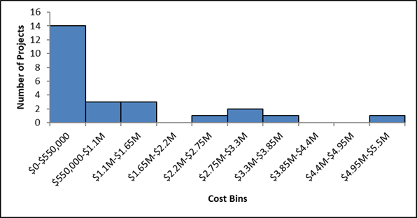
| Cost Bins | Number of Projects |
|---|---|
| $0-$550,000 | 14 |
| $550,000-$1.1M | 3 |
| $1.1M-$1.65M | 3 |
| $1.65M-$2.2M | 0 |
| $2.2M-$2.75M | 1 |
| $2.75M-$3.3M | 2 |
| $3.3M-$3.85M | 1 |
| $3.85M-$4.4M | 0 |
| $4.4M-$4.95M | 0 |
| $4.95M-$5.5M | 1 |
Project costs are skewed to the right with the majority of the projects costing less than $1 million each, and just two projects costing over $3 million. This cost range was taken into consideration when constructing the range of project costs in the analytical scenarios.
Twenty analytical scenarios were developed using three primary sources:
For the purposes of the analysis, it was assumed that the park and ride lots were used exclusively on work days (250 times per year), and that the useful life of the lots was twenty years. Additionally, it was assumed that travelers who utilized the park and ride lot reduced their LDV use by an average of 24 miles (twelve miles each way in the morning and afternoon). Finally, it was assumed that the transit vehicles already operated from the park and ride lot, and therefore no additional transit vehicle emissions were incurred.
Three inputs varied across the twenty scenarios (Table 8 ). The facility and utilization assumptions were based on projects publicized by State DOTs, transit agencies, and local governments.15 The cost data was based on publicized data as well as PAS data.
| Parameter | Value Range |
|---|---|
| Number of Spaces | 100 to 650 spaces |
| Utilization Rate | 40% to 100% |
| Days per Year | 250 days |
| Daily Miles Reduced (per Vehicle) | 24 miles |
| Project Lifetime | 20 years |
| Project Cost | $200,000 to $3.3M |
As an illustrative example, consider a scenario involving a new park and ride lot to encourage transfers from LDV to public transit.
In this scenario, the following assumptions were used:
Step One: Identify annual emissions impacts by multiplying per-trip emissions by the number of affected trips:
| Pollutant | LDV Emissions Reduced (grams/mile) | Daily VMT Reduction | Annual VMT Reduction | Annual Emission Benefit (grams) | Annual Emission Benefit (tons) |
|---|---|---|---|---|---|
| NOx | 0.369 | 9,000 | 2,250,000 | 829,622 | 0.915 |
| PM2.5 | 0.012 | 28,076 | 0.031 |
Step Two: Identify project-level emission impacts by multiplying each of the estimated annual emissions benefits by the project lifetime:
| Pollutant | Annual Emission Benefit (tons) | Project Lifetime (years) | Total Emission Impact (tons) |
|---|---|---|---|
| NOx | 0.915 | 20 | 18.290 |
| PM2.5 | 0.031 | 0.619 |
Step Three: Calculate cost-effectiveness estimates by dividing the project cost by the estimated project-level emission impacts:
| Pollutant | Total Emission Impact (tons) | Project Cost | Cost-effectiveness (dollars per ton) |
|---|---|---|---|
| NOx | 18.290 | $2,000,000 | $109,349 |
| PM2.5 | 0.619 | $3,231,141 |
The median cost-effectiveness estimates for the range of park and ride project scenarios are presented in Table 12 below:
| Project Type | PM2.5 | PM10 | CO | NOx | VOCs |
|---|---|---|---|---|---|
| Park and Ride | $2,660,225 | $732,201 | $7,986 | $90,028 | $131,848 |
Ridesharing projects encourage mode shift from single-occupant LDV to multiple-occupant vehicles (carpools and vanpools). Ridesharing projects may involve direct subsidies of drivers of shared vehicles, the purchase of vanpools and indirect support such as ride-matching services.
This analysis included the following steps:
The PAS contains 40 ridesharing projects identified for this analysis, with a wide variety of purposes: marketing and outreach, operation assistance, pooling of low emission vehicles, and vanpools startup and replacement. The distribution of project costs is shown in Figure 7 below. As mentioned in the previous section, ridesharing projects may involve direct subsidies of drivers of shared vehicles, the purchase of vanpools and indirect support such as ride-matching services. Restricting the subtypes from the PAS based on this definition, the average is about $431,000.
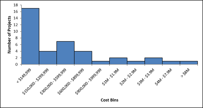
| Cost Bins | Number of Projects |
|---|---|
| < $149,999 | 17 |
| $150,000 - $299,999 | 4 |
| $300,000 - $599,999 | 7 |
| $600,000 - $899,999 | 4 |
| $900,000 - $999,999 | 1 |
| $1M - $1.9M | 2 |
| $2M - $2.9M | 1 |
| $3M - $3.9M | 2 |
| $4M - $7.9M | 1 |
| > $8M | 1 |
In addition, information on ridesharing projects was identified through a review of ridesharing project documentation.16 Using the 2019 operating and capital budget for the Ann Arbor Area Transit Authority's VanRide service as a representative example, vehicle replacement including components averages about $350,000 per year. This cost range was taken into consideration when constructing the range of project costs in the analytical scenarios.
Nine analytical scenarios were developed using the following sources:
For purposes of this analysis, it was assumed that the average reduction in single-occupant trips associated with each rideshare trip is eight (i.e. half of a van's capacity)17. The rideshare trip distance traveled was allowed to vary between 20-40 miles.
| Parameter | Value Range |
|---|---|
| Average reduction of single occupant trips associated with ridesharing | 8 trips |
| Average total distances associated with ridesharing | 160, 240, 320 miles |
| Workdays per Year | 250 days |
| Project Lifetime | 5 years |
| Project Cost | $350K, $400K, $450K |
As an illustrative example, consider a project involving a new ridesharing project.
In this scenario, the following assumptions were used:
Step One: Identify annual emissions impacts by multiplying per-trip emissions by the number of affected trips.
| Pollutant | Emissions Reduced (grams/mile) | Annual VMT Reduction | Annual Emission Benefit (tons) |
|---|---|---|---|
| NOx | 0.3716 | 960,000 | 0.393 |
| PM2.5 | 0.0126 | 0.013 |
Step Two: Identify project-level emission impacts by multiplying each of the estimated annual emission impacts by the project lifetime.
| Pollutant | Annual Emission Benefit (tons) | Project Lifetime (years) | Total Emission Impact (tons) |
|---|---|---|---|
| NOx | 0.393 | 5 | 1.97 |
| PM2.5 | 0.013 | 5 | 0.07 |
Step Three: Calculate cost-effectiveness estimates by dividing the project cost by the estimated project-level emission impacts.
| Pollutant | Lifetime Emission Benefit (tons) | Project Cost | Cost-effectiveness (dollars per ton) |
|---|---|---|---|
| NOx | 1.97 | 400,000 | $203,417 |
| PM2.5 | 0.07 | $6,010,024 |
The median cost-effectiveness estimates for the range of scenarios are presented in Table 17 below:
| Project Type | PM2.5 | PM10 | CO | NOx | VOCs |
|---|---|---|---|---|---|
| Ridesharing | $6,010,024 | $1,667,035 | $17,901 | $203,417 | $295,708 |
For purposes of this report and the CMAQ program, employee transit benefits are functionally identical to subsidized transit fares. Both programs reduce the cost of transit to incentivize its use, thereby diverting LDV trips to transit. Since employee transit benefits are a type of subsidized transit benefit and the methodologies for assessing the cost-effectiveness of such programs are essentially the same, please refer to the subsidized transit fares section of this report for the cost-effectiveness analysis.
Carsharing projects offer access to vehicles owned and maintained by third parties (e.g., cities) for intermittent trips best served by LDVs (LDVs). Shared vehicles provide alternatives to reduce household LDV, and in some cases enable households to own fewer cars, both of which may result in decreases in VMT through eliminating some discretionary trips and mode shift to public transit).
This analysis included the following steps:
The PAS contains eight carsharing projects prior to 2016 identified for analysis. The average was approximately $974,794. The distribution of project costs is shown in Figure 8 below.
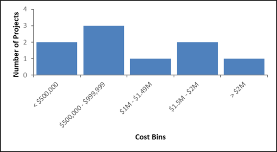
| Cost Bins | Number of Projects |
|---|---|
| < $500,000 | 2 |
| $500,000 - $999,999 | 3 |
| $1M - $1.49M | 1 |
| $1.5M - $2M | 2 |
| > $2M | 1 |
As shown above, the majority of projects cost between $900,000 and $1,500,000. In addition this, information on carsharing projects was identified through a review of carsharing project documentation and supporting literature.18
Nine analytical scenarios were developed using the following sources:
For purposes of this analysis, it was assumed that each shared vehicle is used by fifteen owners of light duty vehicles19, fleet size of 500, and each participant reduces net annual VMT by 2500 to 450020 with average travel speed of 35 mph. Additionally, the useful life of the project is assumed to be five years. Across the nine scenarios, two inputs varied: the annual VMT reduction per person and project costs.
| Parameter | Value Range |
|---|---|
| Number of Owners Sharing LDV | 11 |
| Number of LDV (Fleet Size) | 500 |
| Annual VMT Reduction per person (one way) | 2,500; 3,500; 4,500 |
| Travel Speed | 35 |
| Project Lifetime | 5 years |
| Project Cost | $1M, $1.5M; $2M |
As an illustrative example, consider a project involving a new carsharing project.
In this scenario, the following assumptions were applied:
Step One: Identify annual emissions impacts by multiplying per-miles emissions by the number of affected trips.
| Pollutant | Emission Rates (grams/mile) | Annual VMT Reduction | Annual Emission Benefit (grams) | Annual Emission Benefit (tons) |
|---|---|---|---|---|
| NOx | 0.372 | 27.5M | 10,220,222 | 11.27 |
| PM2.5 | 0.0126 | 27.5M | 345,916 | 0.38 |
Step Two: Each of the estimated annual emissions benefits is multiplied by the project lifetime to identify project-level emission impacts:
| Pollutant | Annual Emission Benefit (tons) | Project Lifetime (years) | Lifetime Emission Benefit (tons) |
|---|---|---|---|
| NOx | 11.27 | 5 | 56.3 |
| PM2.5 | 0.38 | 5 | 1.91 |
Step Three: Divide the project cost by the estimated project-level emission impacts to calculate cost-effectiveness estimates.
| Pollutant | Lifetime Emission Benefit (tons) | Project Cost | Cost-effectiveness (dollars per ton) |
|---|---|---|---|
| NOx | 56.3 | $1,000,000 | 19,020 |
| PM2.5 | 1.91 | $1,000,000 | 561,976 |
The median cost-effectiveness estimates for the range of scenarios are presented in Table 22 below:
| Project Type | PM2.5 | PM10 | CO | NOx | VOCs |
|---|---|---|---|---|---|
| Carsharing | $561,976 | $155,879 | $1,674 | $19,020 | $27,650 |
Bikesharing projects involve providing incentives to shift travel mode from LDV to bicycle for some trips (rather than reducing the number of cars owned by households), by offering access to bicycles owned and maintained by third parties (e.g., cities) for intermittent trips.
This analysis included the following steps:
The PAS contains ten bikesharing projects identified for analysis from 2016. The median project cost was $1,150,793. The distribution of project costs is shown in Figure 9 below.
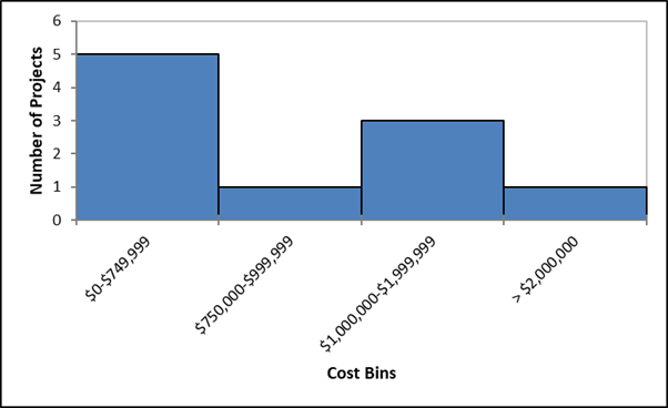
| Cost Bins | Number of Projects |
|---|---|
| $0-$749,999 | 5 |
| $750,000-$999,999 | 1 |
| $1,000,000-$1,999,999 | 3 |
| > $2,000,000 | 1 |
The project costs are slightly bimodal, with the majority of the projects costing less than $1 million and/or between $1-2 million.
Starting a bike share program requires substantial capital.21 Including the cost of fixed infrastructure such as docking stations, systems typically cost about $4,000 to $5,000 per bike. With a typical city funding up to 35 docking stations and about 350 bicycles, total capital investment can reach $1,575,000.22 This cost range was taken into consideration when building and analyzing cost-effectiveness scenarios.
Nine analytical scenarios were developed using the following sources:
For purposes of this analysis, it was assumed that annual ridership ranges from 1,000,000 to 2,000,000 (e.g., annual ridership for Capital Bikeshare in Washington DC is at the high end at 2,000,000)23 and that the average net impact of each trip by shared bicycle is a reduction in travel by light duty vehicle of two miles at 35 miles per hour.24 Additionally, useful life of the project is assumed at five years. Across the nine scenarios, two inputs varied: the number of trips per year via shared bicycle and project cost.
| Parameter | Value Range |
|---|---|
| Travel Length | 2 miles |
| Annual Ridership | 1,000,000; 1,500,000; 2,000,000 |
| Annual VMT Reduction | 200,000; 300,000; 400,000 |
| Project Lifetime | 5 years |
| Project Cost | $750,000; $1,000,000; $1,500,000 |
As an illustrative example, consider a project involving a new bikesharing project. In this scenario, the following assumptions were used:
Step One: Identify Annual Emission Benefit by multiplying per-trip emissions by the number of affected trips.
| Pollutant | Emission Rates (grams/mile) | Annual VMT Reduction | Annual Emission Benefit (grams) | Annual Emission Benefit (tons) |
|---|---|---|---|---|
| NOx | 0.3716 | 2,000,000 | 743,289 | 0.81934 |
| PM2.5 | 0.0126 | 2,000,000 | 25,158 | 0.02773 |
Step Two: Each of the estimated annual emissions benefits is multiplied by the project lifetime to identify project-level emission impacts:
| Pollutant | Annual Emission Benefit (tons) | Project Lifetime (years) | Lifetime Emission Benefit (tons) |
|---|---|---|---|
| NOx | 0.81934 | 5 | 4.09668 |
| PM2.5 | 0.02773 | 5 | 0.13866 |
Step Three: Divide the project cost by the estimated project-level emission impacts to calculate cost-effectiveness estimates.
| Pollutant | Lifetime Emission Benefit (tons) | Project Cost | Cost-effectiveness (dollars per ton) |
|---|---|---|---|
| NOx | 4.09668 | $750,000 | 183,075.18 |
| PM2.5 | 0.13866 | $750,000 | 5,409,021.27 |
The median cost-effectiveness estimates for the range of scenarios are presented in Table 27 below:
| Project Type | PM2.5 | PM10 | CO | NOx | VOCs |
|---|---|---|---|---|---|
| Bikesharing | $5,409,021.27 | $1,500,331.46 | $16,110.94 | $5,409,021.27 | $1,500,331.46 |
These projects involve the provision of electric vehicle charging infrastructure (EVCI) to support the use of electric vehicles in place of conventional LDVs. As with other CMAQ analyses, it was assumed that there are no operational emissions associated with the use of electric vehicles other than brakewear and tirewear as PM.
This analysis included the following steps:
Information on EVCI projects within the PAS was scant: seven EVCI projects were identified between 1992 and 2016. The median project cost was $312,287 (Figure 10 ). Note that this analysis does not differentiate between different electric-vehicle charging types (e.g., DC fast charging, Level 2), because information of different charging types was not available.
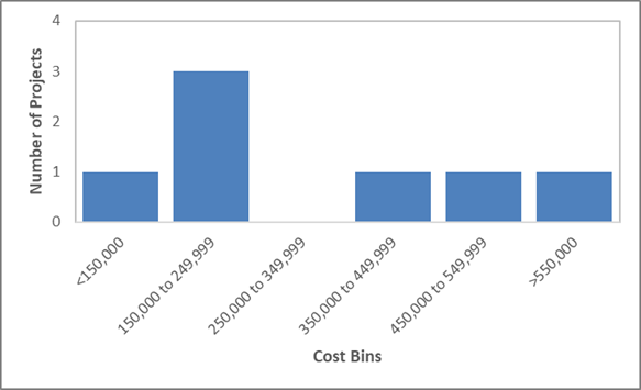
| Cost Bins | Number of Projects |
|---|---|
| < $150,000 | 1 |
| $150,000 - $249,999 | 3 |
| $250,000 - $349,999 | 0 |
| $350,000 - $449,999 | 1 |
| $450,000 - $549,999 | 1 |
| > $550,000 | 1 |
Project costs are slightly skewed to the left, with majority of the projects costing between $150,000 and $249,999. This range does not deviate far from the costs found in published EVCI projects where basic Level 2 charging stations costs $25,000 for the equipment, plus $15,000 installation cost.25 With an average of 5-6 charging stations per parking garage, the typical total cost would lie somewhere between $150,000 and $249,999. This cost range was considered when constructing cost-effectiveness scenarios.
Nine analytical scenarios were developed using the following sources:
For purposes of this analysis, it was assumed that trip length on average is twenty miles, with average travel speeds of 35 mph. Additionally, useful life of the project is assumed to be seven years.26 Different charging station types will be able to charge vehicles at different rates, different configurations will accommodate different numbers of vehicles, and project cost will correspondingly vary as well. Across the nine scenarios, two inputs varied: the number of trip offsets per day due to the presence of EVCI project, which varied between 75 to 150 trips per day; and project cost, which was allowed to vary between $150,000 and $250,000.
As an illustrative example, consider a new EVCI project.
In this scenario, the following assumptions were used:
Step One: Annual emissions benefits are identified by multiplying per-mile emission rates by the number of affected trips under the relevant travel speed, and subtracting the remaining brakewear and tirewear PM:
| Pollutant | Emissions Reduced (grams/mile) | Annual VMT Reduction | Annual Emission Benefit (grams) | Annual Emission Benefit (tons) | |
|---|---|---|---|---|---|
| NOx | 0.3577 | 1,000,000 | 357,665.68 | 0.3943 | |
| PM2.5 | 0.0048 | 1.20665E-5 | 1,000,000 | 7,267.94 | 0.008 |
Step Two: Multiply each of the estimated annual emission benefit by the project lifetime to calculate project-level emission impacts.
| Pollutant | Annual Emission Benefit (tons) | Project Lifetime (years) | Lifetime Emission Impact (tons) |
|---|---|---|---|
| NOx | 0.3943 | 7 | 2.7598 |
| PM2.5 | 0.008 | 7 | 0.0561 |
Step Three: Divide the project cost by the estimated project-level emission impacts to calculate cost-effectiveness estimates.
| Pollutant | Lifetime Emission Impact (tons) | Project Cost | Cost-effectiveness (dollars per ton) |
|---|---|---|---|
| NOx | 2.7598 | $200,000 | $72,468.71 |
| PM2.5 | 0.0561 | $200,000 | $3,566,287.73 |
The median cost-effectiveness estimates for the range of scenarios are presented in Table 31 below:
| Project Type | PM2.5 | PM10 | CO | NOx | VOCs |
|---|---|---|---|---|---|
| Electric Vehicle Charging Infrastructure | $3,566,287.73 | $2,628,699.98 | $6,742.11 | $72,468.71 | $106,381.99 |
Idle reduction strategy projects focus on providing technologies or instituting polices or procedures the reduce vehicle idling emissions. These strategies include truck stop electrification (TSE), retrofitting vehicle power management systems or otherwise upgrading vehicles, and instituting policies in traditionally high-idling areas, such as school or airport drop-off/pick-up areas. Emission impacts were identified as the product of idling emission rates, number of trucks impacted by the reduction strategies, and project lifetimes.
The analyses of scenarios were conducted using outputs from the FHWA CMAQ Emissions Calculator Toolkit, as well as project-level inputs from CMAQ projects and various State Departments of Transportation.27 Emissions benefits were determined using the CMAQ Toolkit. Note this project category and related analysis focus on heavy-duty trucks and do not address passenger vehicles.
This analysis included the following steps:
The PAS contains nine idle reduction strategy projects from 2013 through 2016.28 The median project cost was approximately $704,000. The distribution of projects costs are shown in Figure 11 below.
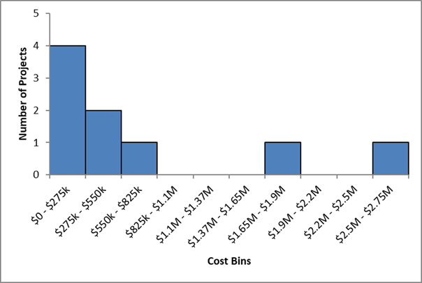
| Cost Bins | Number of Projects |
|---|---|
| $0 - $275k | 4 |
| $275k - $550k | 2 |
| $550k - $825k | 1 |
| $825k - $1.1M | 0 |
| $1.1M - $1.37M | 0 |
| $1.37M - $1.65M | 0 |
| $1.65M - $1.9M | 1 |
| $1.9M - $2.2M | 0 |
| $2.2M - $2.5M | 0 |
| $2.5M - $2.75M | 1 |
The small number of identified projects shows a slight skew to the right with the majority of projects costing less than $700,000. Two larger projects cost $1.9 million and $2.5 million respectively. This cost range was taken into consideration when constructing cost-effectiveness scenarios.
Twenty analytical scenarios were developed using three primary sources:
For the purposes of the analysis, it was assumed that the idle reduction strategies were used exclusively on work days (250 times per year), and that the useful life of the projects was ten years. Additionally, it was assumed that each project would impact a range of trucks, but that the primary power units impacted would use diesel fuel. The cost data was based on publicized data as well as PAS data.
| Parameter | Value Range |
|---|---|
| Number of Trucks Annually Impacted | Distributed Range: 150 to 1,000 |
| Project Lifetime | 10 years |
| Project Cost | $100,000 to $1.75M |
As an illustrative example, consider a scenario involving an idle reduction strategy that upgrades vehicles and reduces idle emissions rates.
In this scenario, we assume the following:
Step One: Identify annual emissions impacts by multiplying per-trip emissions by the number of affected trips.
| Pollutant | Idle Emissions Reduced (kilograms/day) | Annual Reduction | Annual Emission Benefit (kilograms) | Annual Emission Benefit (tons) |
|---|---|---|---|---|
| NOx | 389.007 | 400 Trucks | 97,251 | 107.202 |
| PM2.5 | 5.565 | 1,391 | 1.534 |
Step Two: Identify project-level emission impacts by multiplying each of the estimated annual emissions benefits by the project lifetime.
| Pollutant | Annual Emission Benefit (tons) | Project Lifetime (years) | Total Emission Impact (tons) |
|---|---|---|---|
| NOx | 107.202 | 10 | 1,072 |
| PM2.5 | 1.534 | 15 |
Step Three: Calculate cost-effectiveness estimates by dividing the project cost by the estimated project-level emission impacts:
| Pollutant | Total Emission Impact (tons) | Project Cost | Cost-effectiveness (dollars per ton) |
|---|---|---|---|
| NOx | 1,072 | $400,000 | $373 |
| PM2.5 | 15 | $26,082 |
The median cost-effectiveness estimates for the range of idle reduction strategy project scenarios are presented in Table 36 below:
| Project Type | PM2.5 | PM10 | CO | NOx | VOCs |
|---|---|---|---|---|---|
| Idle Reduction Strategies | $29,450 | $26,187 | $1,017 | $421 | $1,924 |
Bicycle and pedestrian projects provide infrastructure facilitating walking and bicycling in place of travel by LDVs. Sample projects include constructing sidewalks, crosswalks, on-street bikeways, and separated bicycle and walking paths. Cost-effectiveness estimate scenarios assumed no associated public transit service modifications and thus no emission impacts involving public transit: both additional public transit person-trips chained to new bicycle and walking trips and changes from transit to non-motorized trips were assumed to have a negligible effect on transit vehicle emissions.
This analysis included the following steps:
The PAS contains 354 bicycle and pedestrian projects identified for analysis from 2016. The median project cost was approximately $299,251. The distribution of project costs is shown in Figure 12 below.
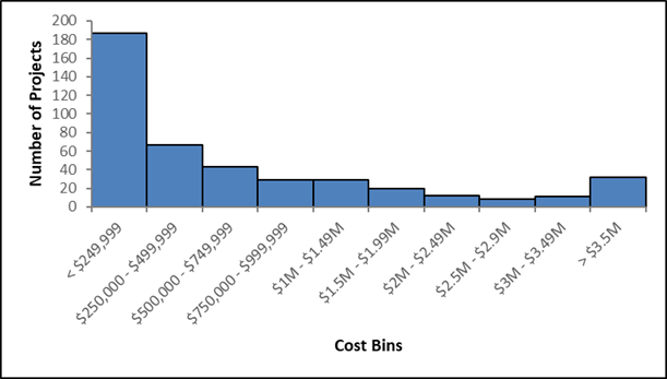
| Cost Bins | Number of Projects |
|---|---|
| < $249,999 | 187 |
| $250,000 - $499,999 | 67 |
| $500,000 - $749,999 | 43 |
| $750,000 - $999,999 | 29 |
| $1M - $1.49M | 29 |
| $1.5M - $1.99M | 20 |
| $2M - $2.49M | 12 |
| $2.5M - $2.9M | 8 |
| $3M - $3.49M | 11 |
| > $3.5M | 32 |
Project costs are skewed to the left, with the majority of the projects costing less than $250,000 each. This compares with national surveys of bicycle and pedestrian infrastructure costs, which find that the average cost of bicycle lanes and multiuse paths is $228,760 per mile.29 This cost range was taken into consideration when constructing cost-effectiveness scenarios.
Nine analytical scenarios were developed using the following sources:
For the purposes of this analysis, it was assumed that average travel speed is at 35 mph, the facilities are used about 250 times per year, and the useful life was at fifteen years. A single round-trip distance of 0.9 miles was assumed based on an analysis of the 2017 National Household Travel Survey (NHTS). 30 This value represents the mean one-way trip distance of the middle 50% of trips taken by walking or bicycling, multiplied by two. This method removed extreme outliers and provides a representative typical trip.
Three inputs varied across the nine scenarios. The daily volume of offset light-duty trips varied between 325, 375, and 425. The 2015 CMAQ assessment study reported an estimated average increase of 374 bike/walk trips per day due to infrastructure.31 Buehler and Pucher reported that modal shifts for 90 large cities in the US was 352 trips per day.32
| Parameter | Value Range |
|---|---|
| Trip shifts from LDV to Bike/Ped | 325; 375; 425 |
| Days Used Per Year | 250 |
| Typical Round-Trip Distance | 0.9 miles |
| Annual VMT Reduction | 162,500; 187,500; 212,500 |
| Travel Speed | 35 mph |
| Project Lifetime | 15 years |
| Project Cost | $200,000; $250,000; $300,000 |
As an illustrative example, consider a new bicycle lane along an existing roadway. In this scenario, the following assumptions were applied:
Step 1: Identify annual emission benefit by multiplying per-trip emissions by the number of affected trips.
| Pollutant | Emissions Reduced (grams/mile) | Annual VMT Reduction | Annual Emission Benefit (grams) | Annual Emission Benefit (tons) |
|---|---|---|---|---|
| NOx | 0.3716 | 84,375 | 31,357.5 | 0.0346 |
| PM2.5 | 0.0126 | 1061.3 | 0.0012 |
Step 2: Multiply each of the estimated annual emission benefit by the project lifetime to calculate project-level emission impacts.
| Pollutant | Annual Emission Benefit (tons) | Project Lifetime | Lifetime Emission Impact (tons) |
|---|---|---|---|
| NOx | 0.0346 | 15 | 0.5185 |
| PM2.5 | 0.0012 | 0.0176 |
Step 3: Divide the project cost by the estimated project-level emission impacts to calculate cost-effectiveness estimates.
| Pollutant | Lifetime Emission Impact (tons) | Project Cost | Cost-Effectiveness (dollars per ton) |
|---|---|---|---|
| NOx | 0.5185 | $250,000 | $482,173 |
| PM2.5 | 0.0176 | $14,245,981 |
The median cost-effectiveness estimates for the range of scenarios are presented in Table 41 below:
| Project Type | PM2.5 | PM10 | CO | NOx | VOCs |
|---|---|---|---|---|---|
| Bike and Pedestrian Projects | $14,245,981 | $3,951,490 | $42,432 | $482,173 | 700,938 |
Freight and intermodal projects focus on providing new options at port facilities for reducing heavy-duty truck trips and encouraging the transfer to rail or other modes, resulting in an emission reduction and also increased capacity and time-savings and more efficient port operations. Emission impacts were identified as the product of per-mile emission rates and activity totals across mitigated heavy-duty-vehicle trips and project lifetimes. Note that this analysis does not include the contribution of emissions from the new mode (e.g., rail or barge), in line with the 2015 cost-effectiveness study. The increase in rail miles or rail hours (or corresponding barge activity) from an intermodal project is difficult to estimate based on the CMAQ Public Access Database. Project sponsors typically report emissions benefits based solely on the number of truck trips diverted and do not subtract emissions from the replacement mode.
In addition, intermodal freight projects may use existing rail lines and vessels to move products and may not require purchase of a new locomotive or marine engine. Therefore, the amount of truck VMT diverted was assumed to provide a reasonable estimate of emission benefits for the analysis. This methodology can potentially be refined given more detailed CMAQ reporting data and mode shift data.
Heavy-duty truck vehicles simulated in this analysis are all assumed to use diesel fuel; on-road vehicle types simulated include both short- and long-haul single-unit and combination trucks. Total emissions and cost-effectiveness comparisons are based on total tonnage and dollars per ton bases.
This analysis included the following steps:
The CMAQ Public Access Database contains sixteen freight and intermodal projects from 2014 through 2016.33 The median project cost was approximately $3.1 million. Fifteen of the sixteen projects were under $7 million in total cost, and one large project was undertaken for $12.5 million. The distribution of projects costs are shown in Figure 13 below.
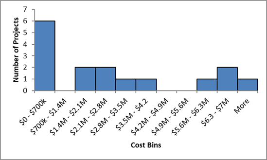
| Cost Bins | Number of Projects |
|---|---|
| $0 - $700k | 6 |
| $700k - $1.4M | 0 |
| $1.4M - $2.1M | 2 |
| $2.1M - $2.8M | 2 |
| $2.8M - $3.5M | 1 |
| $3.5M - $4.2 | 1 |
| $4.2M - $4.9M | 0 |
| $4.9M - $5.6M | 0 |
| $5.6M - $6.3M | 1 |
| $6.3 - $7M | 2 |
| More | 1 |
As shown above, project costs are slightly skewed to the right. While a number of projects were under $700,000, a wide range of projects exists. This is based on the wide range of activities within this project type, which range from crane rehabilitations to major infrastructure construction. This cost range was taken into consideration when building and analyzing the scenarios, which focused on rail infrastructure projects.
Twelve analytical scenarios were developed using three primary sources:
For the purposes of the analysis, it was assumed that the port facilities where the freight and intermodal projects occurred operate year round and the activity is therefore dispersed over 365 days. Additionally it was assumed that the useful life of the projects was twenty years.
Several inputs varied across the twenty scenarios (Table 42). The activity rate assumptions were based on anticipated port operations. The cost data was based on public data as well as PAS data.
| Parameter | Value Range |
|---|---|
| Annual Truck Trips Reduced | Distributed Range: |
| Annual Truck VMT Reduced | Distributed Range: |
| Days per Year | 250 days |
| Project Lifetime | 20 years |
| Project Cost | $800,000 to $1.9M |
As an illustrative example, consider a scenario involving a rail track and switch addition to a port that will encourage transfers from heavy-duty trucks to rail.
In this scenario, we assume the following:
Step One: Identify annual emissions impacts by multiplying per-trip emissions by the number of affected trips:
| Pollutant | Heavy-Duty-Vehicle Emission Mitigation (grams/mile) | Annual VMT Reduction | Annual Emission Impact (grams) | Annual Emission Impact (tons) |
|---|---|---|---|---|
| NOx | 5.605 | 1,500,000 | 8407823.915 | 8.807 |
| PM2.5 | 0.198 | 296328.9471 | 0.276 |
Step Two: Identify project-level emission impacts by multiplying each of the estimated annual emission impacts by the project lifetime:
| Pollutant | Annual Emission Impact (tons) | Project Lifetime (years) | Total Emission Impact (tons) |
|---|---|---|---|
| NOx | 8.807 | 20 | 184.871 |
| PM2.5 | 0.276 | 6.515 |
Step Three: Calculate cost-effectiveness estimates by dividing the project cost by the estimated project-level emission impacts (heavy-duty vehicle emissions reduced):
| Pollutant | Total Emission Impact (tons) | Project Cost | Cost-effectiveness (dollars per ton) |
|---|---|---|---|
| NOx | 184.871 | $1,000,000 | $5,409 |
| PM2.5 | 6.515 | $153,487 |
The median cost-effectiveness estimates for the range of freight and intermodal project scenarios are presented in Table 46 below:
| Project Type | PM2.5 | PM10 | CO | NOx | VOCs |
|---|---|---|---|---|---|
| Freight and Intermodal | $217,360 | $154,839 | $23,677 | $7,661 | $91,297 |
Subsidized transit fare programs seek to stimulate shifts to public transit at times of peak environmental need through the use of temporary discounts on fares, such as during periods with high ozone levels (e.g., ozone action days). The estimated emission impacts centered on travel shifts from LDV to transit. Emission impacts were identified as the product of per-mile emission rates and VMT totals across mitigated LDV trips (less additional bus emissions), and project lifetimes.
This analysis included the following steps:
The PAS contains 21 subsidized transit fare projects identified for analysis from 2016, with a median project cost of approximately $204,000 (Figure 14).34
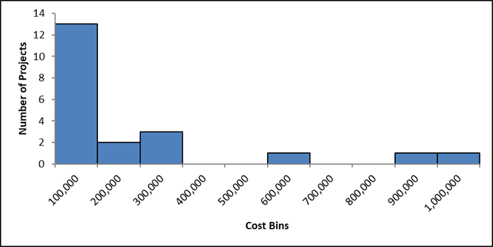
| Cost Bins | Number of Projects |
|---|---|
| 100000 | 13 |
| 200000 | 2 |
| 300000 | 3 |
| 400000 | 0 |
| 500000 | 0 |
| 600000 | 1 |
| 700000 | 0 |
| 800000 | 0 |
| 900000 | 1 |
| 1000000 | 1 |
Project costs are clearly skewed to the right, with the majority of the projects costing less than $200,000 each. Most fare subsidy programs are relatively low in cost compared to other transit projects. The determined cost range was taken into consideration when building and analyzing the scenarios.
Twenty analytical scenarios were developed using three primary sources:
For the purposes of the analysis, it was assumed that travelers who converted to transit reduced their LDV use by, on average, ten miles (five miles each way during the morning and afternoon commutes). Additionally, it was assumed that he programs were funded and operated for three years.
Across the twenty scenarios, three inputs were varied. The number of travelers who converted to transit varied between 4,000 and 6,250 riders. The program was assumed to operate ten days per year, and the project cost was assumed to vary between $50,000 and $900,000.
These assumptions were based on projects publicized by transit agencies (including TriMet and Los Angeles County MTA). Table 47 below shows the scenario parameters and value ranges.
| Parameter | Value |
|---|---|
| Daily Shift to Transit | 4,000 to 6,250 riders |
| Days per Year | 10 days |
| Daily Miles Reduced (per Vehicle) | 10 miles |
| Project Lifetime | 3 years |
| Project Cost | $50,000 to $900,000 |
As an illustrative example, consider a scenario involving a fare-free program for ozone action days.
In this scenario, the following assumptions were used:
Step One: Identify annual emissions benefits by multiplying per-trip emissions by the number of affected trips:
| Pollutant | Emissions Reduced (grams/mile) | Annual VMT Reduction | Annual Emission Benefit (grams) | Annual Emission Benefit (tons) |
|---|---|---|---|---|
| NOx | 0.369 | 398,230 | 146,836 | 0.162 |
| PM2.5 | 0.012 | 4,969 | 0.005 |
Step Two: Multiply each of the estimated annual emissions benefits by the project lifetime to calculate project-level emission impacts:
| Pollutant | Annual Emission Benefit (tons) | Project Lifetime (years) | Total Emission Impact (tons) |
|---|---|---|---|
| NOx | 0.162 | 3 | 0.332 |
| PM2.5 | 0.005 | 0.016 |
Step Three: Divide the project cost by the estimated project-level emission impacts to calculate cost-effectiveness estimates:
| Pollutant | Lifetime Emission Impact (tons) | Project Cost | Cost-effectiveness (dollars per ton) |
|---|---|---|---|
| NOx | 0.332 | $550,000 | $1,132,675 |
| PM2.5 | 0.016 | $33,469,232 |
Table 51 presents the median cost-effectiveness estimates for the range of subsidized transit fare project scenarios:
| Project Type | PM2.5 | PM10 | CO | NOx | VOCs |
|---|---|---|---|---|---|
| Subsidized Transit Fares | $36,926,797 | $10,163,738 | $110,850 | $1,249,687 | $1,830,196 |
Transit service expansion projects encourage mode shift to public transit by increasing the availability of transit service in a given region. Consistent with the full range of projects in the analysis, the entire range of relevant costs were considered when evaluating transit service projects, rather than focusing solely on the subset representing CMAQ funding. The estimated emission impacts reflect modal shifts from LDV to transit. Emission impacts were identified as the product of per-mile emission rates and VMT totals across mitigated LDV trips (less additional bus emissions), and project lifetimes.
This analysis included the following steps:
The PAS contains nine projects identified for analysis from 2016.35 The median project cost was approximately $1.8 million (Figure 15).
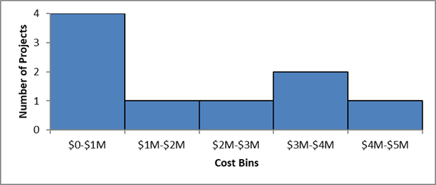
| Cost Bins | Number of Projects |
|---|---|
| $0-$1M | 4 |
| $1M-$2M | 1 |
| $2M-$3M | 1 |
| $3M-$4M | 2 |
| $4M-$5M | 1 |
Project costs are skewed to the right, with the majority of the projects costing less than $1 million each. However, despite the small sample there is a clear range of project costs, up to approximately $5 million. The determined cost range was taken into consideration when building and analyzing the scenarios.
Twenty analytical scenarios were developed using three primary sources:
For the purposes of the analysis, it was assumed that two types of service expansion projects occurred: new transit service bus routes, and increased capacity on existing transit service bus routes. In these scenarios, users would convert to transit exclusively on work days (250 times per year). Light rail projects were not included in the service expansion category.
Five inputs varied across the twenty scenarios (Table 52). For the ten new transit service bus route scenarios, the range of daily travelers shifting to transit was 3,000 to 6,600 riders. The assumed daily LDV miles traveled avoided was 25 miles. The assumed new daily transit bus vehicle miles traveled ranged from 250 to 400. The increase in transit bus vehicle emissions was subtracted from the avoided light-duty emissions. The assumed project lifetime that the expanded service would be funded and operated was five years. The assumed project costs ranged from $1 million to $3.2 million.
For the ten increased capacity scenarios, the range of daily travelers shifting to transit was 1,000 to 1,900 riders. The assumed daily LDV miles traveled avoided was twenty. The assumed project lifetime that the increased capacity would be funded and operated was three years. The assumed project costs ranged from $500,000 to $950,000.
These assumptions were based on projects publicized by State DOTs (including Louisiana DOT), transit agencies (including Nova Transit), and local governments (including Athens-Clarke County, Georgia).
| Parameter | Value |
|---|---|
| Daily Shift to Transit | 3,000 to 6,600 riders for new routes 1,000 to 1,900 riders for increased capacity |
| Days per Year | 250 days |
| Daily Miles Reduced (per Vehicle) | 25 miles for ne555w routes 20 miles for increased capacity |
| Daily New Bus VMT | 350 to 500 miles traveled for new routes 0 miles traveled for increased capacity |
| Project Lifetime | 5 years for new routes 3 years for increased capacity |
| Project Cost | $1M to $3.2M for new routes $500,000 to $950,000 for increased capacity |
As an illustrative example, consider a scenario involving the addition of a new transit route.
In this scenario, the following assumptions were used:
Step One: Identify gross annual emissions benefits by multiplying per-trip LDV emissions by the number of offset trips:
| Pollutant | Emissions Reduced (grams/mile) | Annual LDV VMT Reduction | Annual Emission Benefit (grams) |
|---|---|---|---|
| NOx | 0.369 | 16,592,920 | 6,118,157 |
| PM2.5 | 0.012 | 752,261 |
Step Two: Identify net annual emissions benefits by subtracting new annual bus emissions from the gross annual emissions benefits from Step One:
| Pollutant | Annual Emission Benefit (grams) | New Bus Emissions (grams/mile) | Annual New Bus VMT | Annual New Bus Emissions (grams) | Annual Net Emission Impact (tons) |
|---|---|---|---|---|---|
| NOx | 6,118,157 | 6.138 | 87,500 | 537,064 | 6.152 |
| PM2.5 | 752,261 | 0.154 | 13,487 | 0.213 |
Step Three: Calculate project-level emission impacts by multiplying estimated annual emissions benefits by the project lifetime:
| Pollutant | Annual Net Emission Impact (tons) | Project Lifetime (years) | Lifetime Emission Impact (tons) |
|---|---|---|---|
| NOx | 6.152 | 5 | 30,761 |
| PM2.5 | 0.213 | 1.067 |
Step Four: Estimate cost-effectiveness by dividing the project cost by the estimated project-level emission impacts:
| Pollutant | Lifetime Emission Impact (tons) | Project Cost | Cost-effectiveness (dollars per ton) |
|---|---|---|---|
| CO | 30.761 | $1,000,000 | $32,509 |
| NOx | 1.067 | $937,344 |
Table 57 presents the median cost-effectiveness estimates for the range of transit service expansion project scenarios analyzed:
| Project Type | PM2.5 | PM10 | CO | NOx | VOCs |
|---|---|---|---|---|---|
| Transit Service Expansion | $2,035,198 | $556,301 | $6,029 | $69,251 | $99,652 |
Transit facility and amenity improvement projects focus on enhancing the experience of transit users, in turn shifting travel demand to public transit. Emission impact scenarios modeled the substitution of LDV trips for transit. Emission impacts were identified as the product of per-mile emission rates and VMT totals across mitigated LDV trips (less the additional bus emissions), and project lifetimes.
This analysis included the following steps:
The PAS contains twenty transit amenity improvement projects from 2016, with project costs averaging approximately $24.9 million (Figure 16 ).36
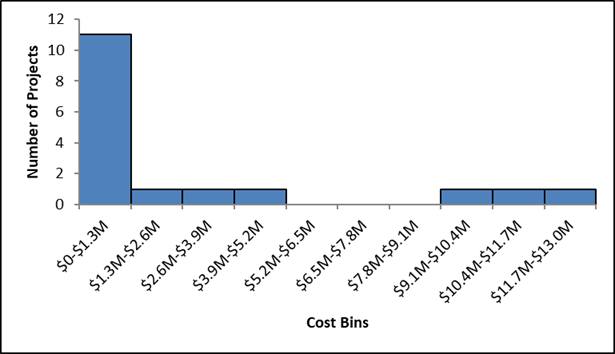
| Cost Bins | Number of Projects |
|---|---|
| $0-$1.3M | 11 |
| $1.3M-$2.6M | 1 |
| $2.6M-$3.9M | 1 |
| $3.9M-$5.2M | 1 |
| $5.2M-$6.5M | 0 |
| $6.5M-$7.8M | 0 |
| $7.8M-$9.1M | 0 |
| $9.1M-$10.4M | 1 |
| $10.4M-$11.7M | 1 |
| $11.7M-$13.0M | 1 |
Project costs are skewed to the right, with the majority of projects costing less than $1 million each. However, there is a very wide range of project costs, with several projects costing over $10 million and two projects costing over $100 million. The two large projects included major vehicle overhauls and installing bus rapid transit facilities. However, since typical amenity improvement projects are less ambitious and therefore cost less, these outliers were not considered when building and analyzing cost-effectiveness scenarios.
Fifteen analytical scenarios were developed using three primary sources:
For the purposes of the analysis, it was assumed that three types of amenity improvement projects occurred: bus stop rehabilitation, improved fare collection systems, and enhanced bicycle and pedestrian connections. These scenarios assume that users would convert to transit exclusively on work days (250 times per year), and that the useful life of the amenities was fifteen years.37 Additionally, it was assumed that travelers who converted to transit and utilized the amenities reduced their LDV use by an average of ten miles (five miles each way in the morning and afternoon).38 Finally, transit vehicles operating with the enhanced amenities were assumed to already be in use, and therefore incurred no additional emissions.
Across the fifteen scenarios, two input were varied: the number of users who shifted, on average, to transit and the project costs (Table 58). For the bus stop rehabilitation scenarios, it was assumed that a range of 100 to 200 users converted to transit per day, at a cost ranging from $140,000 to $500,000. For the improved fare collection systems scenarios, it was assumed that a range of 200 to 300 users converted to transit per day at a cost ranging from $500,000 to $1 million. For the enhanced bicycle and pedestrian connection scenarios, it was assumed that a range of 300 to 400 users converted to transit per day at a cost ranging from $750,000 to $1.4 million. These assumptions were based on available transit literature (Table 58).
| Parameter | Value |
|---|---|
| Daily Shift to Transit | 100 to 200 riders for bus stop rehabilitation 200 to 300 riders for improved fare collection 300 to 400 riders for enhanced connections |
| Days per Year | 250 days |
| Daily Miles Reduced (per Vehicle) | 10 miles |
| Project Lifetime | 10 years |
| Project Cost | $140,000 to $500,000 riders for bus stop rehabilitation $50,000 to $1M riders for improved fare collection $750,000 to $1.4M riders for enhanced connections |
As an illustrative example, consider a scenario involving the installation of a new traveler information system, which would improve users' abilities to time their transfers and make connections.
In this scenario, we assume the following details:
Step One: Identify Annual emissions benefits by multiplying per-trip emissions by the number of affected trips:
| Pollutant | Emissions Reduced (grams/mile) | Daily VMT Reduction | Annual VMT Reduction | Annual Emission Benefit (grams) | Annual Emission Benefit (tons) |
|---|---|---|---|---|---|
| NOx | 0.36872095 | 2,655 | 663,717 | 244,726 | 0.270 |
| PM2.5 | 0.01247836 | 8,282 | 0.009 |
Step Two: Identify project-level emission impacts by multiplying annual emissions benefits by the project lifetime:
| Pollutant | Annual Emission Benefit (tons) | Project Lifetime (years) | Total Emission Impact (tons) |
|---|---|---|---|
| NOx | 0.270 | 15 | 4.046 |
| PM2.5 | 0.009 | 0.137 |
Step Three: Divide the project cost by the estimated project-level emission impacts to calculate cost-effectiveness estimates.
| Pollutant | Total Emission Impact (tons) | Project Cost | Cost-effectiveness (dollars per ton) |
|---|---|---|---|
| NOx | 4.046 | $750,000 | $185,347 |
| PM2.5 | 0.137 | $5,476,783 |
Table 62 presents the median cost-effectiveness estimates for the range of transit amenity improvement project scenarios:
| Project Type | PM2.5 | PM10 | CO | NOx | VOCs |
|---|---|---|---|---|---|
| Transit Amenity Improvements | $5,476,783 | $1,507,431 | $16,441 | $185,347 | $271,445 |
This section reviews the analysis of projects involving improvements to intersections, namely reconstructed or repurposed lanes (i.e., adding left-turn lanes). These projects focus on the use of engineering approaches to improve the flow of traffic through intersections and along corridors. The analyses of scenarios were conducted using outputs from the FHWA CMAQ Emissions Calculator Toolkit and project-level inputs from CMAQ projects and various State departments of transportation.39 Emission rate data were determined using the CMAQ Toolkit.
Distinct to other project types, each of the intersection improvement scenarios involved a reduction in delay, generally improving by one level of service, from E to D or from F to E.40 All together, one hundred scenarios were included in the analysis.
This analysis included the following steps:
The PAS contains 27 intersection reconstruction projects identified for analysis from 2016.41 The identified projects included adding acceleration and deceleration lanes, turning lanes, curb and ramp facilities, diverging interchanges, and/or realignments. The median project cost was approximately $2.2 million. The distribution of projects costs are shown in Figure 12 below.
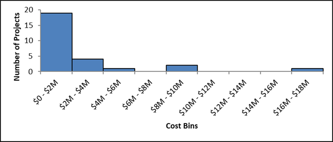
| Cost Bins | Number of Projects |
|---|---|
| $0 - $2M | 19 |
| $2M - $4M | 4 |
| $4M - $6M | 1 |
| $6M - $8M | 0 |
| $8M - $10M | 2 |
| $10M - $12M | 0 |
| $12M - $14M | 0 |
| $14M - $16M | 0 |
| $16M - $18M | 1 |
A majority of the funded intersection improvement projects were under $2 million and focused primarily on adding turn lanes or signals. The distribution skews right, as small number of projects consisted of large reconstruction and corridor-level improvements that included intelligent transportation technology.
One hundred analytical scenarios were developed using four primary sources:
Using the CMAQ Toolkit, a range of input values were needed to determine the scenarios. The range, and the proportion of each value used across the one hundred scenarios, is described in Table 63 below.
| Parameter | Value |
|---|---|
| Area Type | 33% Rural; 67% Urban |
| Business District | 50% Yes; 50% No |
| Peak Hours per Day | 4 hours |
| Existing Intersection Design | 50% Signalized; 50% Unsignalized; 1-3 lanes; No existing turn lanes |
| Average Annual Daily Travel | Distributed Range: 5,000 to 40,000 |
| Peak Hour Volume | Distributed Range: 500 to 3,500 |
| Truck Percentage | 6% |
| Existing Delay | 35 to 50 seconds per vehicle |
| Cycle Length | 90 Seconds |
| Improved Intersection Design | Left turn lanes and phases added; Right turn phases added |
| Project Lifetime | 20 years |
| Project Cost | Distributed Range: $400,000 to $2.8 Million |
As an illustrative example, consider a scenario involving improvements to an urban, single lane, signalized intersection.
In this scenario, the following assumptions were used:
Step One: Improving the average travel speed by adding turn lanes and phases would lead to the following reductions in emissions of NOx and PM2.5:
| Pollutant | Emissions Reduced (kilograms per day) | Lifetime Emission Impact (Tons) |
|---|---|---|
| NOx | 0.282 | 1.482 |
| PM2.5 | 0.021 | 0.111 |
Step Two: Divide the project cost by the estimated project-level emission impacts to calculate cost-effectiveness estimates.
| Pollutant | Lifetime Emission Impact (tons) | Project Cost | Cost-effectiveness (dollars per ton) |
|---|---|---|---|
| NOx | 1.482 | $920,000 | $620,876 |
| PM2.5 | 0.111 | $8,287,586 |
The median cost-effectiveness estimates for the range of intersection improvement scenarios are presented in Table 12 below:
| Project Type | PM2.5 | PM10 | CO | NOx | VOCs |
|---|---|---|---|---|---|
| Intersection Improvement | $13,255,774 | $12,130,195 | $447,858 | $993,075 | $3,685,105 |
These projects focus on the use of engineering approaches to improve the flow of traffic through intersections and along corridors through the construction of roundabouts... The analyses of scenarios were conducted using outputs from the FHWA CMAQ Emissions Calculator Toolkit and project-level inputs from CMAQ projects and various State departments of transportation.42 Emission rate data were determined using the Toolkit.
Similar to the intersection improvement project type, each of the roundabout scenarios involved a reduction in delay. In all, thirty scenarios were included in the analysis.
This analysis included the following steps:
The PAS contains eight roundabout-related projects identified for analysis from 2016.43 The identified projects included adding acceleration and deceleration lanes, turning lanes, curb and ramp facilities, diverging interchanges, and/or realignments. The median project cost was approximately $867,000. The distribution of project costs is shown in Figure 18 below.
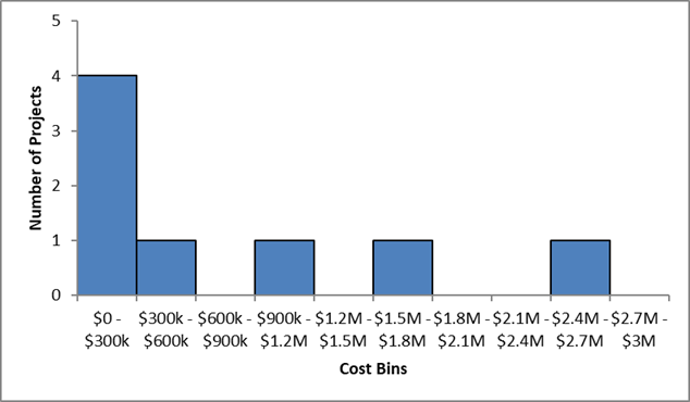
| Cost Bins | Number of Projects |
|---|---|
| $0 - $300k | 4 |
| $300k - $600k | 1 |
| $600k - $900k | 0 |
| $900k - $1.2M | 1 |
| $1.2M - $1.5M | 0 |
| $1.5M - $1.8M | 1 |
| $1.8M - $2.1M | 0 |
| $2.1M - $2.4M | 0 |
| $2.4M - $2.7M | 1 |
| $2.7M - $3M | 0 |
A majority of the funded roundabout projects were under $300,000 and focused primarily on modifying existing, signalized intersections. A small number of projects consisted of larger reconstruction of the existing intersections. Overall, there were only a few very expensive ($2M+) projects, i.e. the distribution is not very skewed. Many projects that included roundabouts also included other activities, which is why a limited number of roundabout only projects (eight total) were available to sample.
Thirty analytical scenarios were developed using four primary sources:
Using the CMAQ Toolkit, a range of input values were needed to determine the scenarios. The range, and the proportion of each value used across the thirty scenarios, is described in the table below.
| Parameter | Value |
|---|---|
| Area Type | 33% Rural; 67% Urban |
| Business District | 50% Yes; 50% No |
| Peak Hours per Day | 4 hours |
| Existing Intersection Design | 50% Signalized; 50% Unsignalized; 3-4 approaches |
| Existing Traffic Flow | Distributed Range: 15%-20% left turns, 25%-85% right turns |
| Average Annual Daily Travel | Distributed Range: 5,000 to 32,000 vehicles |
| Peak Hour Volume | Distributed Range: 400 to 1,700 |
| Truck Percentage | 6% |
| Existing Delay | 55-65 seconds per Vehicle |
| Improved Intersection Design | Distributed Range: 1-2 circulating roundabout lanes; 3-4 approaches |
| Project Lifetime | 20 years |
| Project Cost | Distributed Range: $250,000 to $2.6 million |
As an illustrative example, consider a scenario involving an urban, three-approach, signalized intersection, converted to being a roundabout.
In this scenario, the following assumptions were used:
Step One: Improving the average travel speed from fifteen miles per hour to twenty miles per hour would lead to the following per-mile reductions in emissions of NOx and PM2.5:
| Pollutant | Emissions Reduced (kilograms per day) | Lifetime Emission Impact (Tons) |
|---|---|---|
| NOx | 0.715 | 3.940 |
| PM2.5 | 0.262 | 1.445 |
Step Two: Divide the project cost by the estimated project-level emission impacts to calculate cost-effectiveness estimates.
| Pollutant | Lifetime Emission Impact (tons) | Project Cost | Cost-effectiveness (dollars per ton) |
|---|---|---|---|
| NOx | 3.940 | $1,250,000 | $317,258 |
| PM2.5 | 1.445 | $864,776 |
The median cost-effectiveness estimates for the range of roundabout scenarios are presented in Table 70 below:
| Project Type | PM2.5 | PM10 | CO | NOx | VOCs |
|---|---|---|---|---|---|
| Roundabouts | $1,091,411 | $5,098,858 | $188,255 | $417,433 | $1,549,013 |
This analysis involves the improvement of traffic flow attributed to projects involving traffic signal improvements and synchronization, namely adding traffic signals or synchronizing corridors across several signals. These projects focus on the use of engineering approaches to improve the flow of traffic through intersections and along corridors. The scenario analyses were conducted using outputs from the CMAQ Toolkit and project-level inputs from CMAQ projects and various State departments of transportation.44 Emission rate data were determined using the Toolkit.
Similar to the intersection improvement project type, each of the traffic signal synchronization scenarios involved a reduction in delay. In all, fifty scenarios were included in the analysis.
This analysis included the following steps:
The PAS contains 100 traffic signal-related projects identified for analysis from 2016.45 The identified projects included adding signals or installing a series of synchronized signals over the length of a corridor. The median project cost was approximately $825,000. The distribution of projects costs are shown in Figure 19 below.
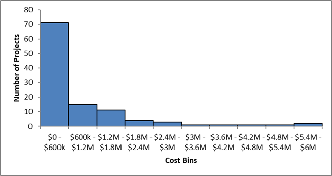
| Cost Bins | Number of Projects |
|---|---|
| $0 - $600k | 71 |
| $600k - $1.2M | 15 |
| $1.2M - $1.8M | 11 |
| $1.8M - $2.4M | 4 |
| $2.4M - $3M | 3 |
| $3M - $3.6M | 1 |
| $3.6M - $4.2M | 1 |
| $4.2M - $4.8M | 1 |
| $4.8M - $5.4M | 1 |
| $5.4M - $6M | 2 |
A majority of the funded signal synchronization projects were under $600,000 and focused primarily on modifying existing signals or adding one to two improved signals. A small number of projects consisted of larger reconstruction and corridor-level improvements that included broader intelligent transportation technology and a large number of signals, skewing the distribution to the right.
Fifty analytical scenarios were developed using four primary sources:
Using the CMAQ Toolkit, a range of input values were needed to determine the scenarios. The range, and the proportion of each value used across the fifty scenarios, is described in the table below.
| Parameter | Value |
|---|---|
| Area Type | 33% Rural; 67% Urban |
| Corridor Length | Distributed Range:2 to 5 |
| Peak Hours per Day | 4 hours |
| Existing Corridor Speed Limit | Distributed Range: 35 to 55 mph |
| Number of Signals | Distributed Range: 2 to 8 |
| Number of Lanes | Distributed Range 1 to 3 |
| Average Annual Daily Travel | Distributed Range: 20,000 to 75,000 (both directions) |
| Peak Hour Volume | Distributed Range: 1,200 to 6,600 (both directions) |
| Truck Percentage | 6% |
| Cycle Length | 90 Seconds |
| Project Lifetime | 20 years |
| Project Cost | Distributed Range: $500,000 to $2.9 million |
As an illustrative example, consider a scenario involving three new signals added along a two-mile urban corridor.
In this scenario, the following assumptions were used:
Step One: Improving the average travel speed by synchronizing the three signals would lead to the following reductions in emissions of NOx and PM2.5
| Pollutant | Emissions Reduced (kilograms per day) | Lifetime Emission Impact (Tons) |
|---|---|---|
| NOx | 0.111 | 0.611 |
| PM2.5 | -0.015 | -0.082 |
Step Two: Divide the project cost by the estimated project-level emission impacts to calculate cost-effectiveness estimates.
| Pollutant | Lifetime Emission Impact (tons) | Project Cost | Cost-effectiveness (dollars per ton) |
|---|---|---|---|
| NOx | 0.611 | $1,250,000 | $2,046,847 |
| PM2.5 | -0.082 | -$15,164,914 |
The median cost-effectiveness estimates for the range of traffic signal synchronization scenarios are presented in Table 74 below:
| Project Type | PM2.5 | PM10 | CO | NOx | VOCs |
|---|---|---|---|---|---|
| Traffic Signal Synchronization | $1,136,071 | $330,188 | $40,868 | $327,263 | $933,170 |
Incident management projects focus on providing equipment or personnel for the purpose of advising or re-routing drivers during incidents of non-recurring congestion. These activities can reduce emissions primarily through reducing the idle time associated with congestion. Emission impacts were identified as the product of per-mile emission rates and VMT totals across mitigated LDV trips, and project lifetimes.
This analysis included the following steps:
The PAS contains 59 incident management projects from 2014 through 2016.46 The median project cost was approximately $1.1 million. However, there were two outliers. While 57 of the incident management projects were under $3.9 million, the final two projects were $11.7 million and $16.6 million respectively. When removing these, two outliers, the median project cost was $648,000. The distribution of projects costs are shown in Figure 20 below.
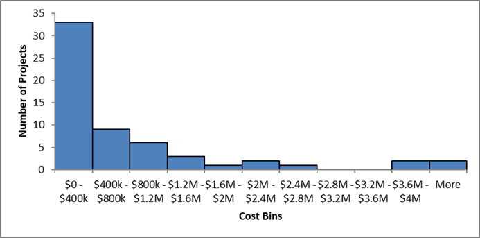
| Cost Bins | Number of Projects |
|---|---|
| $0 - $400k | 33 |
| $400k - $800k | 9 |
| $800k - $1.2M | 6 |
| $1.2M - $1.6M | 3 |
| $1.6M - $2M | 1 |
| $2M - $2.4M | 2 |
| $2.4M - $2.8M | 1 |
| $2.8M - $3.2M | 0 |
| $3.2M - $3.6M | 0 |
| $3.6M - $4M | 2 |
| More | 2 |
Project costs are skewed to the right with the majority of the projects costing less than $800,000 each. This cost range was taken into consideration when constructing cost-effectiveness scenarios.
25 analytical scenarios were developed using three primary sources:
For the purposes of the analysis, it was assumed that the incident management practices are applied to a range of 15 to 35 incidents per year, and that the useful life of the practices was ten years. Additionally, it was assumed that the idle hours reduced per incident ranged from 3,000 to 7,000 hours, across the entire roadway or corridor.47 Finally, it was assumed that the cost ranged from $20,000 to $860,000. The cost data was based on publicized data as well as PAS data.
Table 8 below shows the full range of the scenario parameters.
| Parameter | Value Range |
|---|---|
| Number of Incidents Mitigated per Year | Distributed Range: 15 to 35 |
| Delay Hours Reduced per Incident | Distributed Range: 3,000 to 7,000 |
| Project Lifetime | 20 Years |
| Project Cost | Distributed Range: $20,000 to $860,000 |
As an illustrative example, consider a scenario involving a new incident management system to reduce LDV idle time.
In this scenario, the following assumptions were used:
Step One: Identify annual emissions impacts by multiplying per-trip emissions by the number of affected trips:
| Pollutant | Emissions Reduced (grams) | Annual Idle Hours Reduced | Annual Emission Benefit (grams) | Annual Emission Benefit (tons) |
|---|---|---|---|---|
| NOx | 9.333 | 2,250,000 | 1,119,911 | 1.234 |
| PM2.5 | 0.682 | 81,886 | 0.090 |
Step Two: Identify project-level emission impacts by multiplying each of the estimated annual emissions benefits by the project lifetime:
| Pollutant | Annual Emission Benefit (tons) | Project Lifetime (years) | Total Emission Impact (tons) |
|---|---|---|---|
| NOx | 1.234 | 10 | 12.345 |
| PM2.5 | 0.090 | 0.903 |
Step Three: Calculate cost-effectiveness estimates by dividing the project cost by the estimated project-level emission impacts:
| Pollutant | Total Emission Impact (tons) | Project Cost | Cost-effectiveness (dollars per ton) |
|---|---|---|---|
| NOx | 12.345 | $300,000 | $24,302 |
| PM2.5 | 0.903 | $332,360 |
The median cost-effectiveness estimates for the range of incident management project scenarios are presented in Table 79 below:
| Project Type | PM2.5 | PM10 | CO | NOx | VOCs |
|---|---|---|---|---|---|
| Incident Management | $433,650.54 | $398,231.0068 | $32,994.79 | $31,707.72 | 175,407.00 |
These projects reduce emissions through the replacement of older, high-emission diesel vehicles with new, lower-emission vehicles. A basic example of a relevant vehicle replacement would be replacing an older (model year 2004) diesel truck with a new (model year 2019) truck. Not only would the MY2019 vehicle operate free of the effects of long-term engine wear and tear (unlike the MY2004 engine), but the MY2019 engine would also be designed under more rigorous emission standards for key pollutants such as PM and NOx.
This section replaces heavy-duty engine replacements, due to a lack of real world engine replacement projects funded by the CMAQ program. Within the CMAQ Public Access System from 2014 to 2016, there were only three engine replacement projects reported and 184 vehicle replacement projects. Engine replacements and vehicle replacements have the same emissions impact through the use of new engines and vehicle's with new engines. Note that the costs of a vehicle replacement are higher than an engine replacement, so the cost-effectiveness is lower than that of an engine replacement.
This analysis included the following steps:
The PAS contains 184 vehicle replacement projects from 2014 to 2016 that were identified for analysis. The median cost was approximately $7.4 million However, this median cost represents replacing multiple vehicles, which underscores a data limitation: the PAS reports the project costs but does not specify the number of vehicles replaced. As a result, the cost distribution from the PAS is not reproduced here. The scenarios, example calculations, and the cost-effectiveness values report the cost-effectiveness of replacing a single vehicle as drawn from other sources.
300 analytical scenarios were developed using the following sources:
Note this analysis considers the cost-effectiveness of an individual vehicle replacement, rather than the cost-effectiveness of a given CMAQ project. This analysis focuses on transit and school buses: 89% of the known project types in the PAS were related to school or transit bus replacement. School buses were assumed to all use diesel fuel, while transit buses may either use CNG or diesel. The analysis uses a national activity estimate, in this case VMT, from MOVES2014b for these vehicles. Prices for school buses, CNG transit buses, and diesel transit buses are all based on the literature review. Three replacement cycles are assumed for the vehicles; a low of ten years, a middle of fifteen years, and a high of twenty years.
| Parameter | Value Range |
|---|---|
| Replacement Cycle (years) | 10, 15, 20 |
| Vehicle year | 1999-2018 |
| VMT (annual, 2019) | 8,154, 36,985 |
| Vehicle types | School bus, Diesel transit bus, CNG transit bus |
| Costs | $190,000, $200,000, $300,000 |
As an illustrative example, consider a project involving a new vehicle replacement project (single vehicle).
In this scenario, the following assumptions were applied (on a per-vehicle basis):
Step One: The emissions from the 2019 model are subtracted from the 1999 model to represent the emissions reduction from the project. Annual emission impacts are identified by multiplying the per-mile emission rate mitigation by the representative VMT.
| Pollutant | Emission Rates (grams/mile) | Annual VMT | Annual Emission Benefit (grams) | Annual Emission Benefit (tons) |
|---|---|---|---|---|
| CO | 5.15 | 19,352 | 99,713 | 0.11 |
| PM2.5 | 0.36 | 19,352 | 7,024 | 0.01 |
| PM10 | 0.39 | 19,352 | 7,634 | 0.01 |
| NOx | 15.29 | 19,352 | 295,884 | 0.33 |
| VOCs | 1.42 | 19,352 | 27,456 | 0.03 |
Step Two: Each of the estimated annual emission impacts is multiplied by the project lifetime to identify project-level emission impacts:
| Pollutant | Annual Emission Benefit (tons) | Project Lifetime (years) | Lifetime Emission Benefit (tons) |
|---|---|---|---|
| CO | 0.11 | 20 | 2.2 |
| PM2.5 | 0.01 | 20 | 0.2 |
| PM10 | 0.01 | 20 | 0.2 |
| NOx | 0.33 | 20 | 6.6 |
| VOCs | 0.03 | 20 | 0.6 |
Step Three: The project cost is divided by the estimated project-level emission impacts to yield cost-effectiveness estimates:
| Pollutant | Lifetime Emission Benefit (tons) | Vehicle Cost | Cost-effectiveness (dollars per ton) |
|---|---|---|---|
| CO | 2.2 | $300,000 | $136,468 |
| PM2.5 | 0.2 | $300,000 | $1,937,270 |
| PM10 | 0.2 | $300,000 | $1,782,560 |
| NOx | 6.6 | $300,000 | $45,990 |
| VOCs | 0.6 | $300,000 | $4,187 |
The median cost-effectiveness estimates for the range of scenarios are presented in the table below:
| Project Type | PM2.5 | PM10 | CO | NOx | VOCs |
|---|---|---|---|---|---|
| Vehicle Replacement | $33,942,507 | $31,309,499 | $317,323 | $309,889 | $3,909,224 |
These projects reduce emissions by retrofitting the engines on older diesel vehicles with emissions reduction technologies. A basic example of a relevant diesel engine retrofit would be installing a diesel particulate filter on a MY2002 Combination Long-Haul truck. Diesel particulate filters (DPF) and other emissions technologies reduce some, but not all emissions by capturing them before they can fully exit the exhaust system of the vehicle.
This analysis included the following steps:
The PAS contains 27 diesel retrofit projects identified for analysis from 2014 to 2016. The median cost was approximately $1.4 million. The distribution of project costs shown in below is concentrated in the range between $100,000 and $3,000,000.
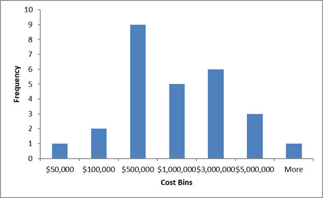
| Cost Bins | Number of Projects |
|---|---|
| $50,000 | 1 |
| $100,000 | 2 |
| $500,000 | 9 |
| $1,000,000 | 5 |
| $3,000,000 | 6 |
| $5,000,000 | 3 |
| More | 1 |
The majority of the projects cost under $1,000,000. In addition, information on diesel projects was validated through a review of engine retrofit project documentation and supporting literature. This cost range was taken into consideration when constructing cost-effectiveness scenarios.
252 analytical scenarios were developed using the following sources:
This analysis builds its scenario around a variety of buses and trucks. The analysis uses a national activity estimate, in this case VMT, from MOVES2014b for these vehicles. The types of retrofit and their mitigation factors are pulled from the CMAQ Toolkit. The range of years for retrofitted vehicles is 1999 to 2006. Note that model year 2007 and later heavy-duty engines are required to include emissions reductions technologies as standard48 and are omitted from this analysis. Vehicles from 2004 to 2006 already have Diesel Oxidization Catalysts (DOCs) and Exhaust Gas Recirculation (EGR) technologies, and thus do not receive those retrofits in any of the analysis' scenarios.
Prices for retrofitted devices reflect literature and EPA sources. Three different cost sources were consulted to build scenarios: an EPA report on the cost-effectiveness of diesel retrofit technology49, a report by the International Council on Clean Transportation50, and a fact sheet developed by the Manufacturers of Emission Control Association.51 The relevant service life for the retrofits depends on vehicle use. However, an analysis of the VMT values and literature yields estimates of five years for the Selective Catalytic Reduction (SCR) technology and eight years for all other technologies.
| Parameter | Value Range |
|---|---|
| Replacement Cycle (years) | 8, except for SCR + DCF (5) |
| Vehicle year | 1999-2006 |
| VMT (annual, 2019) | 5,103-84,649 |
| Vehicle types | Intercity Bus, Transit Bus, School Bus, Single Unit Long-Haul Truck, Combination Long-Haul Truck |
| Costs | DOC + DPF: $6,000 DOC: $750-$1500 DOC + CCV: $4,000 DPF: $5,000-$7,000 EGR + DPF: $18,000 SCR + DPF: $15,000 |
As an illustrative example, consider a project involving a retrofit project.
In this scenario, the following assumptions were used:
Step One: The emissions from the retrofitted vehicle are subtracted from the 2000 pre-retrofit vehicle to represent the mitigated emissions. Annual emission impacts are identified by multiplying the per-mile emission rate mitigation by the representative VMT.
| Pollutant | Emission Rates (grams/mile) | Annual VMT | Annual Emission Benefit (grams) | Annual Emission Benefit (tons) |
|---|---|---|---|---|
| CO | 3.17 | 11,492 | 36,430 | 0.0402 |
| PM2.5 | 0.54 | 11,492 | 6,258 | 0.0069 |
| PM10 | 0.59 | 11,492 | 6,802 | 0.0075 |
Step Two: Each of the estimated annual emission impacts is multiplied by the project lifetime to identify project-level emission impacts:
| Pollutant | Annual Emission Benefit (tons) | Project Lifetime (years) | Lifetime Emission Benefit (tons) |
|---|---|---|---|
| CO | 0.0402 | 8 | 0.322 |
| PM2.5 | 0.0069 | 8 | 0.055 |
| PM10 | 0.0075 | 8 | 0.060 |
Step Three: The project cost is divided by the estimated project-level emission impacts to yield cost-effectiveness estimates.
| Pollutant | Lifetime Emission Benefit (tons) | Project Cost | Cost-effectiveness (dollars per ton) |
|---|---|---|---|
| CO | 0.32 | $6,000 | $18,680 |
| PM2.5 | 0.05 | $6,000 | $108,723 |
| PM10 | 0.06 | $6,000 | $100,026 |
The median cost-effectiveness estimates for the range of scenarios are presented in the table below:
| Project Type | PM2.5 | PM10 | CO | NOx | VOCs |
|---|---|---|---|---|---|
| Diesel Retrofits | $165,130 | $151,919 | $14,671 | $22,133 | $53,831 |
The analysis of extreme-temperature cold-start (ETCS) technologies projects center on the use of technologies to mitigate the inefficiencies of starting vehicles at low temperatures; for the purposes of this analysis, the relevant temperature range was from -40 degrees to zero degrees Fahrenheit.
The most prevalent technology with supporting information useful for analysis was engine block heaters, which serve as the representative technology in the analysis. Engine block heaters are a plug-in device that warms engines above ambient temperature, resulting in vehicle start emissions comparable to starts under non-extreme conditions.
In the analysis, the effects of ETCS projects were investigated at the fleet-average level for a range of vehicle types, including:
The central emission information for the analysis came from MOVES runs, which reported emission rates for vehicles at startup (in grams per start), by vehicle type and ambient temperature (-40, -20 and zero degrees Fahrenheit), and estimates of the effectiveness of relevant technologies from Alaskan projects involving block heaters. National average fleet composition estimates by vehicle type were used to seed the analysis, to represent an assumption that users of block heaters would be distributed consistently with the composition of the national vehicle fleet. In all, 132 ETCS scenarios were analyzed.
Key variables to account for within the analysis include ambient (extreme cold) temperature and the amount of time vehicles are out of operation before starting (i.e., the soak time). Three alternative ambient temperatures were selected (in degrees Fahrenheit): 0, -20, and -40, the latter of which represents the lower bound of expected cold start conditions within the United States (i.e., winter in Fairbanks, Alaska). The upper bound of soak time (greater than 12 hours) was selected for the analysis, to represent cold starts following overnight parking. Estimates of emission reductions under the use of block heaters were identified by multiplying cold-start emission rates (per start) from MOVES by estimates of the number of cold starts per year and estimates of proportional reductions in emissions from cold-start technologies, as identified in a project involving the Municipality of Anchorage (reductions of up to 60%).
This analysis included the following steps:
The CMAQ Public Access Database contains 30 ETCS technologies from 1999 to 2016.52 The projects relating to ETCS technologies ranged from education and incentive programs, operating assistance, retrofitting, and installation of block heaters. As described in the previous section, we are only interested in engine block heater programs. The median project cost was approximately $448,000. The distribution of projects costs are shown in Figure 22 below.
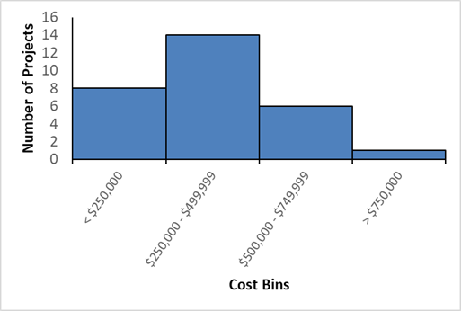
| Cost Bins | Number of Projects |
|---|---|
| < $250,000 | 8 |
| $250,000 - $499,999 | 14 |
| $500,000 - $749,999 | 6 |
| > $750,000 | 1 |
As shown above, project costs are slightly skewed to the left with the majority of the projects costing between $250,000 and $749,999. Four of the PAS entries have listed the quantity of engine block heaters being installed. Calculating per unit cost gives the range $250-$550. This per unit average found in the PAS does not deviate too far from the market average of $200 to $300.53 This cost range was taken into consideration when constructing cost-effectiveness scenarios.
The analysis relies on MOVES estimates of emission rates (in grams per start) for each of the pollutants in the study, by vehicle type and ambient temperature, using national-average travel profiles. The estimated annual impacts on pollutants were identified by multiplying the estimated effectiveness of ETCS technologies (e.g., a 50-percent reduction in PM2.5 emissions at startup) by the number of cold starts per year and the per-start emission rates by vehicle type and ambient temperature.
Lower- and upper-bound values for usage rates (60 and 120 annual cold starts), project lifetime (ten years), and project costs ($250, $500 and $750 per block heater) were used in effectiveness estimates.
To estimate individual cost-effectiveness for each vehicle type/ambient temperature combination in the analysis, the estimated cost for a given project was divided by the sum of estimated annual emission impacts across project lifetimes. Each estimated annual emission impact was identified as the product of the estimated change in a given emission rate (i.e., with the use of ETCS technology versus without) and the assumed annual volume of cold starts for vehicles. This yields a value of dollars per gram of pollutant abated over the project lifetime, which can then be converted to dollars per ton abated.
Thirty-two analytical scenarios were developed using three primary sources:
As an illustrative example, consider the use of a block heater for a passenger vehicle, making 120 starts in -40°F weather. In this scenario, we assume the following details:
Step One: Using a block heater during 120 -40 degree starts would lead to the following annual reductions in emissions of NOx and PM2.5:
| Pollutant | Emission Reduction from Block Heater | Baseline Idle Emission Rate (grams/start) | Annual Cold Starts | Annual Reduction in Emissions from Block Heater (grams) |
|---|---|---|---|---|
| NOx | 40% | 1.23616611 | 120 | 59.336 |
| PM2.5 | 40% | 0.90816188 | 120 | 43.592 |
Step Two: Each of the estimated annual emission impacts is multiplied by the project lifetime to identify project-level emission impacts:
| Pollutant | Annual Reduction in Emissions from Block Heater (grams) | Project Lifetime (years) | Lifetime Reduction in Emissions from Block Heater (tons) |
|---|---|---|---|
| NOx | 59.336 | 10 | 0.00065 |
| PM2.5 | 43.592 | 0.00048 |
Step Three: The project cost is divided by the estimated project-level emission impacts to yield cost-effectiveness estimates:
| Pollutant | Block Heater Cost | Lifetime Reduction in Emissions from Block Heater (tons) |
Cost-effectiveness (dollars per ton) |
|---|---|---|---|
| NOx | 250 | 0.00065 | $1,700,984.52 |
| PM2.5 | 250 | 0.00048 | $4,714,771.41 |
The median cost-effectiveness estimates for the range of extreme-temperature cold-start (ETCS) technologies projects scenarios are presented in the table below:
| Project Type | PM2.5 | PM10 | CO | NOx | VOCs |
|---|---|---|---|---|---|
| ETCS | $4,714,771.41 | $4,170,907.57 | $35,410.39 | $1,700,984.52 | $227,960.51 |
Dust mitigation projects make use of chemical stabilization for dust suppression on unpaved surfaces, or pave previously unpaved surfaces to reduce fugitive dust emissions. Though paving can reduce emissions for other pollutants, since both types are directed at dust emissions, this analysis only reports effects on PM2.5 and PM10. The analyses of scenarios were conducted using outputs from the FHWA CMAQ Emissions Calculator Toolkit and project-level inputs from CMAQ projects and various State Departments of Transportation.54 Emission rate data were determined using the CMAQ Toolkit. The tool was made available to the analysis team for this use only. Note that street sweeping was not considered in the dust mitigation analysis.
This analysis included the following steps:
The PAS contains nine dust mitigation projects identified for analysis involving chemical stabilization or dust suppression from 2014 to 2016.55 The median project cost was approximately $293,000. The distribution of projects costs are shown in Figure 23 below.
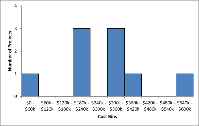
| Cost Bins | Number of Projects |
|---|---|
| $0 - $60k | 1 |
| $60k - $120k | 0 |
| $120k - $180k | 0 |
| $180k - $240k | 3 |
| $240k - $300k | 0 |
| $300k - $360k | 3 |
| $360k - $420k | 1 |
| $420k - $480k | 0 |
| $480k - $540k | 0 |
| $540k - $600k | 1 |
The limited number of chemical stabilization dust mitigation projects funded by the CMAQ program from 2014 to 2016 is fairly normally distributed. The average cost of $293,000 approximates the midpoint of the distribution reasonably well.
Ten analytical scenarios were developed using the following primary sources:
An average annual VMT on unpaved roads of 98,000 was determined based on the Wyoming LTAP study, which showed a mean average daily traffic count (ADT) of 269, or 98,000 annually.
Using the CMAQ Toolkit, a range of input values were needed to determine the scenarios. The range, and the proportion of each value used across the one hundred scenarios, is described in the table below.
| Parameter | Value |
|---|---|
| Annual VMT | Average of 98,000 |
| Vehicle Speed | Distributed Range: 20 mph to 39 mph (based on roadway type) |
| Unpaved Surface Silt Content | Gravel (6.4% Silt Content) or Dirt (11% Silt Content) |
| Unpaved Surface Moisture Content | Typical (1.1% Moisture Content) |
| Dust Control Type | Chemical Stabilization |
| Control Strategy Efficiency | Chemical Treatment (0.8 Efficiency Factor) |
| Project Lifetime | 5 years |
| Project Cost | Distributed Range: $100,000 to $550,000 |
As an illustrative example, consider a scenario involving chemical suppression of a rural, five mile, gravel roadway.
In this scenario, the following assumptions were used:
Step One: Applying chemical stabilization to a gravel roadway would lead to the following reductions in emissions of PM2.5 and PM10:
| Pollutant | Emissions Reduced (kilograms per day) | Lifetime Emission Impact (Tons) |
|---|---|---|
| PM2.5 | 7.95 | 16.02 |
| PM10 | 79.84 | 160.6 |
Step Two: Divide the project cost by the estimated project-level emission impacts to calculate cost-effectiveness estimates.
| Pollutant | Lifetime Emission Impact (tons) | Project Cost | Cost-effectiveness (dollars per ton) |
|---|---|---|---|
| PM2.5 | 16.02 | $250,000 | $15,623 |
| PM10 | 160.6 | $1,556 |
The median cost-effectiveness estimates for the range of dust mitigation scenarios are presented in the table below:
| Project Type | PM2.5 | PM10 | CO | NOx | VOCs |
|---|---|---|---|---|---|
| Dust Mitigation | $14,487 | $1,445 | - | - | - |
These projects involve the provision of natural gas fueling infrastructure (NGFI) projects. NGFI projects have hypothesized impacts on PM2.5, PM10 and VOCs, by encouraging shifts in heavy-duty vehicle travel from diesel-powered vehicles to lower-emission, natural-gas-fueled vehicles. Shifting travel to vehicles fueled by natural gas may lead to increases in NOx emissions, limiting the useful scope of NGFI projects to areas either without the need to curb NOx emissions or with projects with offsetting NOx reductions sufficient to offset NOx increases under NGFI.
This analysis included the following steps:
The PAS contains 66 NFGI projects from 2015 and 2016 identified for analysis. The median project cost was $2,071,942. The distribution of project costs is shown in Figure 24 below.
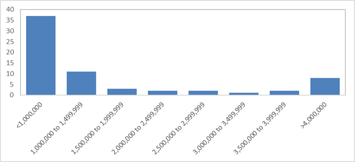
| Cost Bins | Number of Projects |
|---|---|
| <1,000,000 | 37 |
| 1,000,000 to 1,499,999 | 11 |
| 1,500,000 to 1,999,999 | 3 |
| 2,000,000 to 2,499,999 | 2 |
| 2,500,000 to 2,999,999 | 2 |
| 3,000,000 to 3,499,999 | 1 |
| 3,500,000 to 3,999,999 | 2 |
| >4,000,000 | 8 |
Project costs are skewed to the left, with majority of the projects costing between $1,000,000 and $4,000,000. This falls within the bounds identified in a literature review: costs for installing a CNG fueling station can range up to $1.8 million depending on the size and application, and constructing a liquefied natural gas (LNG) fueling site can cost between $1-4 million. This cost range was taken into consideration when constructing cost-effectiveness scenarios.
Nine analytical scenarios were developed using the following sources:
This analysis assumes that the average travel speed of CNG buses as 35 mph. Additionally, the useful life of the project is assumed to be twenty years.
Across the nine scenarios, three inputs varied: the number of transit buses switching from diesel to natural gas, miles traveled by NG buses per year and project cost.
As an illustrative example, consider a project involving a new natural gas fueling station, targeted at serving local buses.
In this scenario, the following assumptions were applied:
Step One: The annual emission impact per vehicle is identified by multiplying per-mile emission impacts per vehicle by the number of vehicles that switch to natural gas due to the project, and the number of miles traveled per vehicle per year:
| Pollutant | Emission Impact per Bus (grams/mile) | Annual VMT per Bus | Annual Number of Affected Trucks | Annual Emission Benefit (grams) | Annual Emission Benefit (tons) |
|---|---|---|---|---|---|
| PM2.5 | 0.036 | 40,000 | 20 | 28,802.5 | 0.03175 |
| PM10 | 0.0407 | 40,000 | 20 | 32,559 | 0.03589 |
Step Two: The estimated annual emission impact is multiplied by the project lifetime to identify project-level emission impacts:
| Pollutant | Annual Emission Benefit (tons) | Project Lifetime (years) | Lifetime Emission Benefit (tons) |
|---|---|---|---|
| PM2.5 | 0.03175 | 20 | 0.63499 |
| PM10 | 0.03589 | 20 | 0.7178 |
Step Three: The project cost is divided by the estimated project-level emission impact to yield the cost-effectiveness estimate:
| Pollutant | Lifetime Emission Benefit (tons) | Project Cost | Cost-effectiveness (dollars per ton) |
|---|---|---|---|
| PM2.5 | 0.63499 | 1.5 M | 2,362,257.45 |
| PM10 | 0.7178 | 1.5 M | 2,089,709.60 |
The median cost-effectiveness estimates for the range of CNG projects scenarios are presented in Table 4 below:
| Project Type | PM2.5 | PM10 | CO | NOx | VOCs |
|---|---|---|---|---|---|
| CNG | 1,866,475.02 | 1,651,128.57 | 9,413.00 | 19,701.68 | 128,388.44 |
23 U.S.C. 149(i)(2) (n.d.).
Aber, Judah. "Electric Bus Analysis for New York City Transit." Columbia University, 2016.
"About TheRide," n.d. https://www.theride.org/AboutUs.
"APTA Statistical Reports." American Public Transportation Association, 2017. https://www.apta.com/resources/statistics/Pages/OtherAPTAStatistics.aspx.
Battelle, and Texas A&M Transportation Institute. "Air Quality and Congestion Mitigation Measure Outcomes Assessment Study: Final Technical Report." Washington DC: US Federal Highway Administration, September 2014. https://www.fhwa.dot.gov/environment/air_quality/cmaq/research/outcomes_assessment/technical_report/index.cfm.
Beitsch, Rebecca. "Despite Popularity, Bike Share Programs Often Need Subsidies." Pew Charitable Trusts, March 24, 216AD. https://www.pewtrusts.org/en/research-and-analysis/blogs/stateline/2016/03/24/despite-popularity-bike-share-programs-often-need-subsidies.
"Benefit-Cost Analysis Guidance for Discretionary Grant Programs." Office of the Secretary, US Department of Transportation, December 2018.
Bliss, Laura. "Here's How Many Cars This Car-Sharing Service Killed." CityLab, July 20, 2016. https://www.citylab.com/transportation/2016/07/car2go-car-ownership-vmt-ghg/491825/.
Buehler, R, and J Pucher. "Cycling to Work in 90 Large American Cities: New Evidence on the Role of Bike Paths and Lanes." Transportation 39, no. 2 (2012): 409–32.
Bushell, Max, Bryan Poole, Charles Zegeer, and Daniel Rodriguez. "Costs for Pedestrian and Bicyclist Infrastructure Improvements." University of North Carolina - Chapel Hill: UNC Highway Safety Research Center, October 2013.
"Capital Bikeshare: System Data," n.d. https://www.capitalbikeshare.com/system-data.
"Certification Procedure for Light-Duty and Heavy-Duty Diesel Vehicles and Heavy-Duty Diesel Engines Using Selective Catalyst Reduction (SCR) Technologies." US Environmental Protection Agency, March 27, 2007. https://iaspub.epa.gov/otaqpub/display_file.jsp?docid=16677&flag=1.
Cervero, R, A Golub, and B Nee. "City CarShare: Longer-Term Travel Demand and Car Ownership Impacts." Transportation Research Record: Journal of the Transportation Research Board, 2007, 70–80.
Chang, Daniel, Daniel Erstad, Ellen Lin, Alicia Falken Rice, Chia Tzun Goh, and An-An Tsao. "Financial Viability Of Non-Residential Electric Vehicle Charging Stations." UCLA Luskin Center for Innovation, August 2012. https://luskin.ucla.edu/sites/default/files/Non-Residential%20Charging%20Stations.pdf.
"CMAQ Emissions Calculator Toolkit." US Federal Highway Administration, n.d. https://www.fhwa.dot.gov/environment/air_quality/cmaq/toolkit/.
"CMAQ Interim Program Guidance." US Department of Transportation Federal Highway Administration, November 2012.
"CMAQ Public Access System." US Federal Highway Administration, n.d. https://fhwaapps.fhwa.dot.gov/cmaq_pub/.
"Congestion Mitigation and Air Quality Improvement (CMAQ) Program." US Federal Highway Administration, n.d. https://www.fhwa.dot.gov/environment/air_quality/cmaq/.
"Congestion Mitigation and Air Quality Improvement (CMAQ) Program: Public Transportation." US Federal Highway Administration, October 4, 2014. https://www.fhwa.dot.gov/Environment/air_quality/cmaq/reference/cmaq_public_transportation/.
"Conversion Factors for Hydrocarbon Components." Washington DC: US Environmental Protection Agency Office of Mobile Sources, 1997.
Duranton, Gilles, and Matthew Turner. "The Fundamental Law of Road Congestion: Evidence from US Cities." American Economic Review 101, no. 6 (October 2011): 2616–52. https://doi.org/DOI: 10.1257/aer.101.6.2616.
Economic and Planning Systems, Inc. "Draft Report: City of Santa Monica Bicycle Sharing Analysis." The City of Santa Monica, CA, October 25, 2012. https://www.smgov.net/uploadedFiles/Departments/PCD/Plans/Bike-Action-Plan/SantaMonicaBikeShare%20cost%20and%20revenue%20estimates.pdf.
"Emissions Factors for Locomotives." Washington DC: US Environmental Protection Agency Office of Mobile Sources, 1997. https://nepis.epa.gov/Exe/ZyPDF.cgi/P1001Z8C.PDF?Dockey=P1001Z8C.PDF.
Energetics Incorporated, Clean Communities of Central New York, and Ithaca-Tompkins County Transportation Council. "Tompkins County Plug-in Electric Vehicle Infrastructure Plan." New York State Energy Research and Development Authority, November 2016. http://tompkinscountyny.gov/files2/itctc/projects/EV/Tompkins%20EVSE%20Site%20Suitability%20FINAL.pdf.
"Highway Capacity Manual: Level of Service Reference Table, Exhibit 21-2." AASHTO, 2010.
"Kitsap Transit: How Many People Does It Take to Form a Vanpool?" Kitsap Transit, n.d. http://www.kitsaptransit.com/faqs/vanpool-frequently-asked-questions/how-many-people-does-it-take-to-form-a-vanpool-this-is-not-a-joke.
Kubsh, Joseph. "Diesel Retrofit Technologies and Experience for On-Road and Off-Road Vehicles." International Council on Clean Transportation, 2017.
"Large Scale EV Charging Infrastructure." Freewire Technologies, February 2016. http://static1.squarespace.com/static/53685b5ce4b05a1adcd370dd/t/5706c48a37013ba79b1e3c34/1460061327999/FreeWire_Charging+Infrastructure+Guide.pdf.
Martin, Elliot, and Susan Shaheen. "The Impacts of Car2go on Vehicle Ownership, Modal Shift, Vehicle Miles Traveled, and Greenhouse Gas Emissions: An Analysis of Five North American Cities." Transportation Sustainability Research Center - UC Berkeley, July 2016. http://innovativemobility.org/wp-content/uploads/2016/07/Impactsofcar2go_FiveCities_2016.pdf.
"NHTS 2009." US Bureau of Transportation Statistics, n.d. https://nhts.ornl.gov/.
"NHTS 2009: Average Vehicle Occupancy by Mode and Purpose." US Bureau of Transportation Statistics, 2009. https://nhts.ornl.gov/tables09/fatcat/2009/avo_TRPTRANS_WHYTRP1S.html.
"Public Electric Vehicle Charging Infrastructure." Sustainable Jersey, June 2017. http://www.sustainablejersey.com/actions-certification/actions/?type=1336777436&tx_sjcert_action%5BactionObject%5D=521&tx_sjcert_action%5Baction%5D=getPDF&tx_sjcert_action%5Bcontroller%5D=Action&cHash=e136260b594094a98ecb6f78df43448a.
Smith, Margaret, and John Gonzalez. "Costs Associated With Compressed Natural Gas Vehicle Fueling Infrastructure." US Department of Energy, September 2014. https://afdc.energy.gov/files/u/publication/cng_infrastructure_costs.pdf.
Suutari, Amanda. "Flexcar: A Model of For-Profit Carsharing." The Eco-Tipping Point Project, 2006. http://www.ecotippingpoints.org/our-stories/indepth/usa-portland-flexcar-carsharing.html.
US Environmental Protection Agency. "Basic Information about Carbon Monoxide (CO) Outdoor Air Pollution | Carbon Monoxide (CO) Pollution in Outdoor Air | US EPA." Accessed August 7, 2018. https://www.epa.gov/co-pollution/basic-information-about-carbon-monoxide-co-outdoor-air-pollution.
---. "Basic Information about Ozone | Ozone Pollution | US EPA." Accessed August 7, 2018. https://www.epa.gov/ozone-pollution/basic-information-about-ozone.
---. "NOx: How Nitrogen Oxides Affect the Way We Live and Breathe." US Environmental Protection Agency Office of Air Quality, September 1998. https://web.archive.org/web/20080716063437/http:/www.epa.gov/air/urbanair/nox/noxfldr.pdf.
---. "Particulate Matter (PM) Basics | Particulate Matter (PM) Pollution | US EPA." Accessed August 7, 2018. https://www.epa.gov/pm-pollution/particulate-matter-pm-basics#PM.
"Volatile Organic Compounds Emissions." US Environmental Protection Agency, 2014. https://cfpub.epa.gov/roe/indicator_pdf.cfm?i=23.
1 Other programs, such as the EPA's Diesel Emissions Reduction Act (DERA) funding programs, also support projects that improve air quality by reducing diesel emissions. These other programs have also analyzed the effectiveness of projects similar to those funded by the CMAQ Program, using their own methods and data. As a result, they may have found different results. Readers are encouraged to consult the DERA Program for additional information: https://www.epa.gov/cleandiesel
2The 2013 Interim Guidance details project eligibility for the CMAQ program: "CMAQ Interim Program Guidance" (US Department of Transportation Federal Highway Administration, November 2012).
3 The median is a measure of central tendency; it is most appropriate to use when data is skewed (asymmetrical distribution) or contains outliers. The median is calculated as the middle value in a range of values ordered from smallest to largest. If there is an even number of observations, the median is the average of the two middle values. The median was chosen instead of the mean for the cost-effectiveness analysis, as many project type costs were skewed to the right or left. Skewedness can significantly distort the mean.
4 Note empty (white) cells in the table indicate that those pollutants do not apply to the particular strategy (e.g., empty cells for CO, NOx, and VOCs with dust mitigation projects). The table is divided into thirds to indicate strong, mixed, and weak overall cost-effectiveness (total median cost-effectiveness across all pollutants).
5 For example, for purposes of this analysis based on MOVES estimated emissions rates, a 2019 model year CNG transit bus produces 84% more kilograms per mile of CO and 33% more kilograms per mile of VOCs than a diesel bus. Conversely, the same CNG bus produces 76% fewer kilograms per mile of PM2.5.
6 Some projects eligible for CMAQ funding have the effect of reducing roadway congestion, such as incident management and intermodal freight facilities. However, 23 U.S.C 149 specifies that project eligibility is confined to transportation projects in non-attainment or maintenance areas that are likely to contribute to attainment or maintenance of a NAAQS.
7 "Benefit-Cost Analysis Guidance for Discretionary Grant Programs" (Office of the Secretary, US Department of Transportation, December 2018).
8 "NHTS 2009: Average Vehicle Occupancy by Mode and Purpose" (US Bureau of Transportation Statistics, 2009), https://nhts.ornl.gov/tables09/fatcat/2009/avo_TRPTRANS_WHYTRP1S.html.
9 Note that this analysis examined a three-legged roundabout, the representative median scenario based on PAS data.
10 "Congestion Mitigation and Air Quality Improvement (CMAQ) Program" (US Federal Highway Administration, n.d.), https://www.fhwa.dot.gov/environment/air_quality/cmaq/.
11 "CMAQ Public Access System" (US Federal Highway Administration, n.d.), https://fhwaapps.fhwa.dot.gov/cmaq_pub/.
12 For more information on the CMAQ Toolkit, please visit the Toolkit website: https://www.fhwa.dot.gov/environment/air_quality/cmaq/toolkit/
13 FHWA 2008, op. cit., p. 55.
14 2016 was chosen as it was the most recent year with full available data.
15 Agencies included Virginia DOT, Sound Transit (WA), the Delaware Transit Corporation, and the Lee County (FL) Board of County Commissioners.
16 "About TheRide," n.d., https://www.theride.org/AboutUs.
17 http://www.kitsaptransit.com/faqs/vanpool-frequently-asked-questions/how-many-people-does-it-take-to-form-a-vanpool-this-is-not-a-joke
18 R Cervero, A Golub, and B Nee, "City CarShare: Longer-Term Travel Demand and Car Ownership Impacts," Transportation Research Record: Journal of the Transportation Research Board, 2007, 70–80; Amanda Suutari, "Flexcar: A Model of For-Profit Carsharing" (The Eco-Tipping Point Project, 2006), http://www.ecotippingpoints.org/our-stories/indepth/usa-portland-flexcar-carsharing.html.
19 Laura Bliss, "Here's How Many Cars This Car-Sharing Service Killed," CityLab, July 20, 2016, https://www.citylab.com/transportation/2016/07/car2go-car-ownership-vmt-ghg/491825/.
20 Elliot Martin and Susan Shaheen, "The Impacts of Car2go on Vehicle Ownership, Modal Shift, Vehicle Miles Traveled, and Greenhouse Gas Emissions: An Analysis of Five North American Cities" (Transportation Sustainability Research Center - UC Berkeley, July 2016), http://innovativemobility.org/wp-content/uploads/2016/07/Impactsofcar2go_FiveCities_2016.pdf.
21 Rebecca Beitsch, "Despite Popularity, Bike Share Programs Often Need Subsidies" (Pew Charitable Trusts, March 24, 216AD), https://www.pewtrusts.org/en/research-and-analysis/blogs/stateline/2016/03/24/despite-popularity-bike-share-programs-often-need-subsidies.
22 Economic and Planning Systems, Inc., "Draft Report: City of Santa Monica Bicycle Sharing Analysis" (The City of Santa Monica, CA, October 25, 2012), https://www.smgov.net/uploadedFiles/Departments/PCD/Plans/Bike-Action-Plan/SantaMonicaBikeShare%20cost%20and%20revenue%20estimates.pdf.
23 "Capital Bikeshare: System Data," n.d., https://www.capitalbikeshare.com/system-data.
24 "NHTS 2009" (US Bureau of Transportation Statistics, n.d.), https://nhts.ornl.gov/.
25 "Public Electric Vehicle Charging Infrastructure" (Sustainable Jersey, June 2017), http://www.sustainablejersey.com/actions-certification/actions/?type=1336777436&tx_sjcert_action%5BactionObject%5D=521&tx_sjcert_action%5Baction%5D=getPDF&tx_sjcert_action%5Bcontroller%5D=Action&cHash=e136260b594094a98ecb6f78df43448a; Energetics Incorporated, Clean Communities of Central New York, and Ithaca-Tompkins County Transportation Council, "Tompkins County Plug-in Electric Vehicle Infrastructure Plan" (New York State Energy Research and Development Authority, November 2016), http://tompkinscountyny.gov/files2/itctc/projects/EV/Tompkins%20EVSE%20Site%20Suitability%20FINAL.pdf.
26 Daniel Chang et al., "Financial Viability of Non-Residential Electric Vehicle Charging Stations" (UCLA Luskin Center for Innovation, August 2012), https://luskin.ucla.edu/sites/default/files/Non-Residential%20Charging%20Stations.pdf.
27 CMAQ project data from the PAS was queried and analyzed. A sample of recent intersection improvement projects was collected from State DOTs through internet research. These data were used to calibrate the analytical scenarios tested.
28 2016 was chosen as it was the most recent year with full available data.
29 Max Bushell et al., "Costs for Pedestrian and Bicyclist Infrastructure Improvements" (University of North Carolina - Chapel Hill: UNC Highway Safety Research Center, October 2013).
30 Federal Highway Administration. (2017). 2017 National Household Travel Survey, U.S. Department of Transportation, Washington, DC. Available online: https://nhts.ornl.gov.
31 Battelle and Texas A&M Transportation Institute, "Air Quality and Congestion Mitigation Measure Outcomes Assessment Study: Final Technical Report" (Washington DC: US Federal Highway Administation, September 2014), https://www.fhwa.dot.gov/environment/air_quality/cmaq/research/outcomes_assessment/technical_report/index.cfm.
32 R Buehler and J Pucher, "Cycling to Work in 90 Large American Cities: New Evidence on the Role of Bike Paths and Lanes," Transportation 39, no. 2 (2012): 409–32.
33 2016 was chosen as it was the most recent year with full available data.
34 2016 was chosen as it was the most recent year with full available data.
35 2016 was chosen as it was the most recent year with full available data.
36 2016 was chosen as it was the most recent year with full available data.
37 "Minimal Asset Useful Life Standards for FTA Grants" (Virginia Department of Rail and Public Transportation, November 30, 2015), https://olga.drpt.virginia.gov/documents/forms/DRPT%20Asset%20Useful%20Life%20Chart.pdf.
38 This assumption relied on a similar analysis of the 2017 NHTS as used in the Bicycle and Pedestrian Improvement Projects section, focused instead on transit trips.
39 CMAQ project data from the PAS was queried and analyzed. A sample of recent intersection improvement projects was collected from State DOTs through internet research. These data were used to calibrate the analytical scenarios tested.
40 "Highway Capacity Manual: Level of Service Reference Table, Exhibit 21-2" (AASHTO, 2010).
41 2016 was chosen as it was the most recent year with full available data.
42 CMAQ project data from the PAS was queried and analyzed. A sample of recent traffic signal synchronization projects was collected from State DOTs through internet research. These data were used to calibrate the analytical scenarios tested.
43 2016 was chosen as it was the most recent year with full available data.
44 CMAQ project data from the PAS was queried and analyzed. A sample of recent traffic signal synchronization projects was collected from State DOTs through internet research. These data were used to calibrate the analytical scenarios tested.
45 2016 was chosen as it was the most recent year with full available data.
46 2016 was chosen as it was the most recent year with full available data.
47 Assumptions on hours reduced per incident derived from the SHRP2 Traffic Incident Management Responder Training Program Final Report: https://www.fhwa.dot.gov/publications/research/randt/evaluations/18038/18038.pdf
48 U.S. EPA's heavy-duty engine standards require use of emission control technologies for model years 2007 and later (40 CFR 86.007-11: Emission standards and supplemental requirements for 2007 and later model year diesel heavy-duty engines and vehicles).
49 U.S. EPA (2007). An Analysis of the Cost-Effectiveness of Reducing Particulate Matter Emissions from Heavy-Duty Diesel Engines Through Retrofits. https://nepis.epa.gov/Exe/ZyPDF.cgi/900N0800.PDF?Dockey=900N0800.PDF
50 International Council on Clean Transportation (2017). Diesel Retrofit Technologies and Experience for On-road and Off-road Vehicles. https://theicct.org/sites/default/files/publications/Diesel-Retrofits_ICCT_Consultant-Report_13062017_vF.pdf
51 Manufacturers of Emission Control Association (MECA). (2011). Diesel Retrofit Frequently Asked Questions http://www.meca.org/galleries/files/DieselRetrofitFAQ_0106.pdf
52 2016 was chosen as it was the most recent year with full available data.
53 https://community.cartalk.com/t/engine-block-heaters/88063/4
54 CMAQ project data from the PAS was queried and analyzed. A sample of recent dust mitigation projects was collected from State DOTs through internet research. These data were used to calibrate the analytical scenarios tested.
55 2016 was chosen as it was the most recent year with full available data.
56 Wyoming University Transportation Center (2019). Assessing the Cost-Effectiveness of Wyoming's CMAQ Unpaved Road Dust Suppression Program, Year 2. https://www.ugpti.org/resources/reports/downloads/mpc19-386b.pdf
U.S. EPA (2002). Estimating Statewide Vehicle Activity and Roadway Mileage for Unpaved Roads in California. https://ww3.arb.ca.gov/research/apr/reports/99-715.pdf

