Linking Transportation and Land Use
Mike McKeever, Sacramento Area Council of Governments
Bruce Griesenbeck, Sacramento Area Council of Governments
Introduction
Linking transportation and land use refers to the process of guiding development and expansion of communities with the goal of better coordination of land use and transportation that accommodates pedestrian and bike safety, mobility, enhances public transportation service, improves road network connectivity, and includes a multi-modal approach to transportation. Typically, this is accomplished through supporting land-use development patterns to create a variety of transportation options.
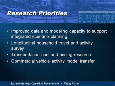
Under increasing pressure from population expansion, development of large tracks of open lands into residential subdivisions or strip-style commercial shops is occurring in communities throughout the United States. At the same time that roads are being widened and new roads are being constructed, the facets of transportation such as bike trails, sidewalks, and other facilities that link activities and users are lagging. The objective of linking transportation and land use is to define and manage this growth of communities in a fashion that balances land use and transportation needs. To achieve this objective, there are a number of important resources that need to be available to planners. The following discusses four priority areas where federal research is needed to support the linkage between transportation and land use.
Improved Data and Modeling Capacity to Support Integrated Scenario Planning
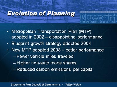
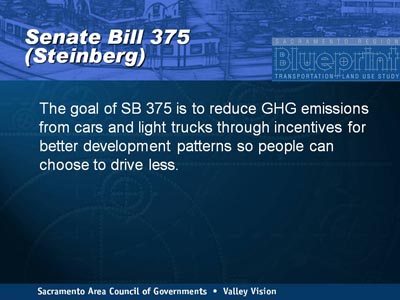
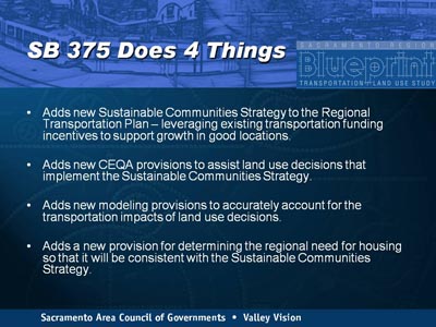
Metro, the Portland (Oregon) regional government, adopted a long-range growth vision in the mid 1990s1. That action spawned a number of regional-scale scenario planning exercises around the country, starting in Utah with Envision Utah, and most recently becoming a statewide Blueprint Planning program sponsored by the California Department of Transportation for all of the regions throughout that large state. The process became popular enough in California that this Fall the state legislature passed and the Governor signed SB375, a landmark law that requires regional planning agencies to integrate climate change, transportation, land use, and housing planning2. There are several initiatives to advocate for inclusion of some of the concepts in SB375 in the new Federal Transportation bill, which is just starting the re-authorization process. FHWA has actively encouraged Metropolitan Planning Organizations (MPOs) to engage in scenario planning activities that integrate transportation, land use, and air quality decisions.
Most of the regional scenario planning initiatives share the following characteristics:
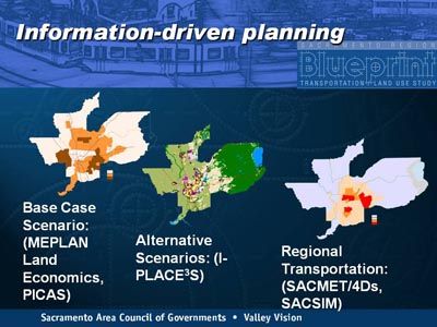
- They use more and more sophisticated data, models, and analysis to estimate the trade offs and impacts of growth decisions on a broadening array of variables, including travel behavior, air emissions, water quality, demand and supply, habitat and natural resources, agriculture, infrastructure costs, floodplains, environmental justice, affordable housing, economic development, and even health.
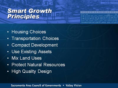
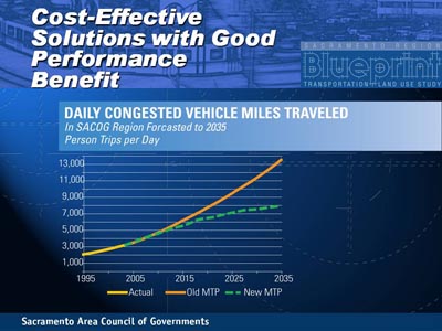
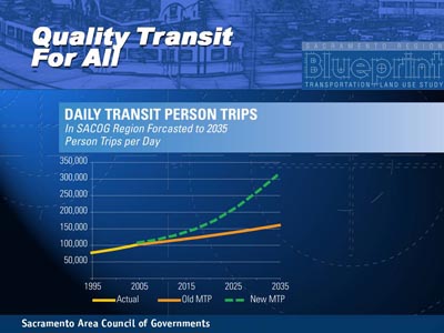
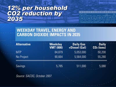
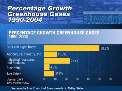
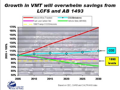
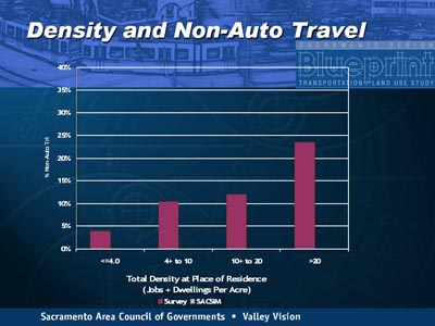
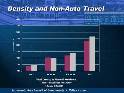
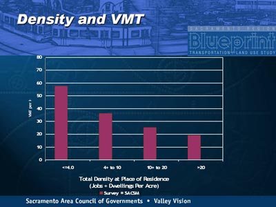
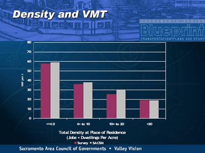
- They almost always result in adopted growth strategies that use compact development, mixed use, transit and pedestrian-oriented design, and other smart principles to reduce per capita vehicle miles traveled and air emissions (including greenhouse gases), increase non-auto trips (transit, walk, bike), and reduce the impact of urbanization on agricultural, habitat, and natural resource lands.
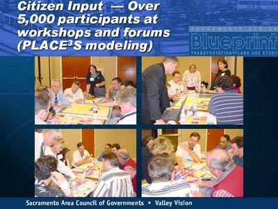
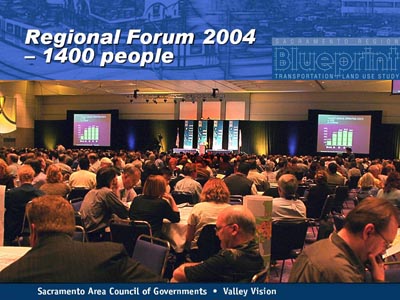
- The planning processes educate large numbers of citizens and stakeholders about complex technical planning issues, and engage the participants in hands-on, interactive mapping exercises (sometimes aided by the use of laptop computers “live” in public meetings) that help citizens understand the full range of impacts of planning choices and build consensus across usually disparate interests and groups.
The Metropolitan Planning Region (MPO) is the most cost-effective scale to build that data, and create modeling and analysis tools necessary to adequately support serious planning. The local level is too small and costly, the state level often is too big and unwieldy in the Western states and too small in the Eastern states. While the MPO is the right scale to build a parcel-level geographic information system, forecasting tools, scenario building models (including three-dimensional visualization capability), and travel and air emissions forecasting models, it still takes money and management-level commitment to make it happen. Many of the technical tools and methods should not be different from one region to another. Some standardization would help cut costs, increase the reliability of results, and support good inter-regional planning to address the cross-border impacts.
Longitudinal Household Travel and Activity Survey
Household travel surveys have advanced in recent years to include important information on the activities that people engage in during the course of the day. Additional data and collection procedures are needed to provide a robust dataset of the transportation and land-use characteristics that influence travel choices. The resulting data set will serve as a cost-effective basis to develop a transferable protocol for activity-based travel models throughout the country.
Traditionally, the surveys were concerned only with the number and location of vehicle and transit trips, then walk and bicycle trips were added. These surveys focused on the primary purpose of the trip as discrete decisions made by travelers, then linking trips into tours was examined to begin to understand how people and households decide on a set of activities and their relative importance.
The locations of trips traditionally was concerned only with the Travel Analysis Zone (TAZ) of the trip, then exact addresses and locations were collected as research pointed out that travel decisions for transit and non-motorized trips depended on very small units of distance and time (i.e., feet not miles, and small not large numbers of minutes).
The surveys traditionally did not collect any information about the location of trips other than TAZ, then research concluded that geographic information about each destination is important to understanding why that location was chosen. The land-use and travel-choice characteristics that influence location choices include street pattern, density and mix of surrounding uses, transit and pedestrian system characteristics, and safety and security among other features.
Originally, the surveys were conducted for only 1 or 2 days for each respondent, but household activities are often scheduled across a week or more for some important mandatory and discretionary trips. Only one survey (in the Puget Sound region) has conducted a multi-year longitudinal survey. By tracking changes in travel and activity over years the long-term behavioral patterns can be analyzed and incorporated into models.
Traditionally, no information was collected on the health of the respondents. More recently, the relationship between land use, transportation system, and health has been examined. Health data include the amount of physical activity, especially walking, exposure to air toxics from vehicles, and personal safety.
Conducting surveys has become more difficult for several reasons. People are more wary of surveys because telemarketers and criminals have used the primary recruitment for household surveys, which are telephone calls to the home. Also, cell phones are now a common, if not the predominate, communication device that makes random household selection within the survey area more difficult. With more attention to detailed spatial data have come concerns about privacy. The surveys have had a requirement that the person and household's private information was not released. Now that it is possible to know the exact address of each trip of each person, attaching the person's name and other vital information is more likely.
Revising the protocols for household travel surveys would address each of these issues in meeting its objectives of a comprehensive survey of urban travel behavior; such a study currently is being planned in California. Key features of the California study include:
- A five or more year survey, with a week of data collected from each respondent each year. The activity and travel data would be collected with both a diary format and with a handheld GPS unit with capability of menu-based data entry. An interview would be done each year that includes data on demographics (including health data), housing, economic information, and travel costs. Stated preference data would be collected on travel and activity choices that are related to options available but not chosen, such as alternate shopping and recreation locations, or travel response to different costs of travel.
- The survey would be repeated to the same households each year for 5+ years. A replacement protocol would be used for households that drop out of the survey.
- The survey would be conducted in 3-5 urban areas that represent a range of urban and suburban development patterns and transportation systems with at least 1,000 households per area.
- Each trip location would be examined for the land use and travel characteristics near it. Land-use density and mix, street pattern, transit service level, and pedestrian system data would be collected for ¼- and ½-mile radius around each location.
Transportation Cost and Pricing Research
An improved travel survey could be used in conjunction with activity-based travel models to better understand the long- and short-term impacts of costs in travel choices.
Part 1 – Exogenous Costs: Vehicle acquisition, disposition, and use study. Using the first wave or two of the longitudinal study described above, estimate model of vehicle acquisition, disposition, and use. This would make it possible to capture the full range of operating costs of different vehicle types, plus the intra-household dynamics of who uses what vehicle for what trips. This would make it possible to actually model the true costs of vehicle transportation (rather than single-point averages), and it would net significant data on vehicle activity by type of vehicle for use in emissions modeling.
Part 2 – Pricing Policy: Modifications to travel models to allow for evaluation of pricing (HOT lanes, toll roads, parking pricing, road pricing). Parts 1 and 2 together would provide the first comprehensive treatment of true transportation costs using an activity-based modeling system for household-based travel.Commercial Vehicle Activity Model Transfer
This would be a unique research effort focused on the transferability of a commercial vehicle/freight activity model from one region to another. The “donor” region would be Calgary, Alberta, Canada. Research would focus on model structural modification and calibration to fit in the Sacramento test region and any other test regions in the country. By implementing this model, SACOG would have the first true activity-based demand simulation model for both household- and commercial-based travel.
Workshop Presentation
1 2040 Growth Concept, Portland Regional Government Metro Council, 1995.
2 California Senate Bill 375, Signed into California Law September 30, 2008.