• Federal Highway Administration >
• Publications >
• Research Publications >
• 05083 >
• Appendd.Cfm
• Appendix D. Wind Tunnel Testing of Stay Cables

Previous | Table of Contents | Next

Appendix D. Wind Tunnel Testing of Stay Cables

EXECUTIVE SUMMARY

To clarify the dry cable galloping phenomenon and verify the instability data by Saito et al., a series of wind tunnel tests of a 2D sectional model of an inclined cable was conducted.⁽¹³⁾ The wind tunnel tests were performed in the propulsion wind tunnel at the Montreal Road campus of the NRC-IAR. The main findings of the current study can be summarized as follows:

• Limited-amplitude high-speed vortex shedding excitations have been observed under a variety of conditions.
• Motions that reached the limits of the test rig were observed at low damping for one case (i.e., 2C); it is possible that this was a divergent galloping instability.
• The limited-amplitude vibration was observed only in the limited wind speed range at different wind speed levels corresponding to the critical Reynolds number. The maximum amplitude of the response depends on the orientation angle of the cable.
• The limited-amplitude high-speed vortex excitation was easily suppressed by increasing structural damping.
• If wind blows along the cable, for cables with a vertical inclination angle θ ≤ 45°, the increase of surface roughness makes the unstable range shift to lower wind speeds.
• Since elastic bands were used to change the frequencies of the cable motion in the X- and Ydirections, which at the same time affects the system damping, no clear frequency ratio effect was identified from the test results. However, this parameter could be important for the aerodynamic behavior of the inclined dry cable, and thus is worthy of further investigation.
• The instability data for inclined cable vibration defined by Saito et al. is found to be more conservative than the results obtained from the current study. The instability defined by the current findings has a much steeper slope than that given by Saito.⁽¹³⁾
• The Reynolds number effect, which results from the model surface condition and the orientation angle, needs to be further explored.

INTRODUCTION

The focus of the test program was to examine the response of a dry cable (i.e., no rain/wind interaction) inclined at various angles to the wind. As discussed in the main text, various methods for suppressing rain/wind oscillations have been developed and appear to be effective, even though not all aspects of the excitation mechanism are fully understood. Therefore, tests on rain/wind excitation were concluded to be not at the top of the priority list. However, the question of oscillations of dry cables is still the subject of much debate. Some believe the only dry cable oscillations that occur are due to parametric excitation, in which the fluctuating aerodynamic forces acting on the deck and towers cause some oscillations of those components, which then feed energy into the cables causing them to develop much larger oscillations. Others believe wind action on the cables themselves, either involving Den Hartog-type galloping or a high-speed form of vortex excitation, is the source of oscillations. The aim of the test program was to investigate the direct action of wind on dry inclined cables with a view toward helping to resolve the debate. In particular, the tests would duplicate some of the conditions tested by Saito et al. and attempt to confirm or modify the criteria suggested in that paper for dry cable galloping.⁽¹³⁾

Since the wind speeds where oscillations have been observed and the typical stay cable diameters result in the cables being in a critical range of Reynolds number (where the aerodynamic parameters such as drag coefficient and Strouhal number undergo rapid transformations), it was important to undertake the testing in the same Reynolds number range as experienced in the field. The “model” scale was therefore selected to be approximately 1:1. A segment of cable with an overall diameter of 160 mm (6.3 inches) was selected (the outer PE sheath, without a spiral bead, being the same as that used for the Maysville Bridge). The test cable mass was selected to facilitate achieving realistic Scruton numbers. Also, it was important to use a wind tunnel with a speed range similar to the range of wind speeds seen on bridges. The propulsion wind tunnel at the NRC in Ottawa, Canada, was selected for this purpose, having a speed range of 0–39 m/s (0– 87 mi/h), and having working section dimensions of 6.1 m (20 ft) in the vertical direction and 3.05 m (10 ft) in the horizontal direction. The local assistance of Professor Hiroshi Tanaka and his graduate student S.H. Cheng at the University of Ottawa was also obtained for the running of the tests, data analysis, and assistance in report preparation. The testing also benefited from the advice and experience of NRC staff, including Dr. Guy Larose who had undertaken tests previously in Europe on cable vibration problems.

The dynamic test rig supporting the test cable was designed and constructed and shipped to Ottawa after initial shake down tests in Guelph. The contractor’;s staff also directed the test program. In designing the rig, use was made of the fact that, in the context of cable vibrations, wind does not know the difference between the vertical and horizontal directions. The only angle that matters as far as its interaction with a cable is concerned is the angle between the wind vector and the cable axis. This simplified the wind tunnel tests because it implied that the test cable could be maintained in a vertical plane aligned with the central axis of the wind tunnel. The only angle adjustment needed to cover the range of relative angles between wind and cable seen on a real bridge was the angle of the test cable to the horizontal. However, a cable on a bridge does have slightly different frequencies in the vertical plane and in lateral direction. Therefore, to the extent that this frequency ratio matters, it was felt that there should be the ability to alter the cable frequencies in two orthogonal directions on the model. This was made possible by having adjustable sets of orthogonal springs at each end of the test cable. The orientation of the test rig springs could be rotated to any angle about the test cable axis. This, combined with the adjustable angle between test cable and the horizontal axis of the wind tunnel, allowed various combinations of wind direction relative to the bridge axis and full scale cable angle relative to the horizontal to be simulated, covering most of the range of interest.

Other parameters of importance to cable vibrations, besides those already discussed, are the damping ratio, frequency ratio of vertical and horizontal cable frequencies, and the surface roughness. Therefore the test program included an examination of the influence of these parameters.

MODEL DESIGN

Cable Model

A 6.7-m (22-ft)-long full-scale cable model was used for the purpose of the current project. The cable, consisting of an inner steel pipe and outer smooth PE tube, has an outside diameter of 160 mm (6.2 inches). A 3/8–16 machine screw was put on at one end only during the initial setup stage to prevent the inner steel pipe sliding out of the PE tube. The weight of the cable itself is 356.4 kg (785 lb), i.e., 53.2 kg/m (35.7 lb/ft). The model is supported on a rig designed and manufactured by RWDI. When the cable vibrates, the effective cable mass should include that of the steel shaft at the pipe ends, and one-third of the spring mass on the supporting rig. Thus, the total active dynamic mass of the cable is 407.4 kg (896 lb), and the effective mass per cable length is 60.8 kg/m (40.8 lb/ft).

Angle Relationships Between the Cable and Mean Wind Direction

As shown in figure 38, the orientation of the cable with respect to the mean wind direction can be represented by two angles. If the wind blows with a horizontal angle of β to the bridge axis, the projection of the cable on the horizontal plane makes a horizontal yaw angle β with the wind vector. Also, if the cable is assumed to be in a vertical plane parallel to the bridge axis, it has a vertical inclination angle θ.

Figure 38. Drawing. Angle relationships between stay cables and natural wind (after Irwin et al.).⁽²⁷⁾

The relative angle Φ between the wind direction and cable axis has the relationship with θ and β as shown in equation 39:

(39)

The direction of cable motion is normal to both the wind direction and the cable axis, and can be represented by the vector θβ´ given in figure 41. θβ´ has an angle α with respect to its horizontal projection θβ. This angle α also has a relationship with the orientation angles θ and β, given by equation 40:

(40)

Supporting Rig

The cable supporting rig was designed and built for the current project by the contractor. For the purpose of the test, there are a number of requirements for the design of the rig:

• To allow the vibration of a 6.7-m (22-ft)-long, 356.4-kg (784.1-lb) full-scale cable model at the natural frequency of 1–2 Hz.
• To allow the convenient change of cable orientation angles for exploring more different setup cases.
• This setup of the cable model allowed for approximately 6.0-m (19.7-ft) of the 6.7-m (22-ft) cable in the wind flow and maintained the upwind support out of the wind flow.
• To keep the inherent structural damping of the whole system as low as possible, so that the level of damping for controlling dynamic behavior can be examined by supplying additional damping.
• To be able to simulate a slight difference between the horizontal and vertical frequencies as it is expected of in the case of real stay cables.

The designed test rig meets all these requirements. It consists of the upper and bottom parts to support both ends of the cable model, as shown in figures 39 and 40. There are two pairs of springs set in two perpendicular directions on each part of the rig. Both springs are in the plane perpendicular to the cable axis. The adjustment of the spring stiffness controls the change in cable frequencies in the spring direction. The total mass of the springs is 60 kg (132 lb). The vertical spring constant is 4.99 kN/m (342 lb/ft), and the horizontal one is 4.78 kN/m (328 lb/ft) (when one of them is placed horizontally).

Figure 39. Photo. Cable supporting rig: Top.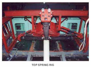

Figure 40. Photo. Cable supporting rig: Bottom.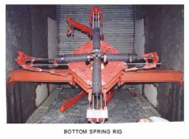

Because of the size of the cable model and the limitation in the dimension of the wind tunnel facility, the simulation of real cable orientation angles, θ and β, for the range of interest is difficult to reproduce. Thus, the simulation of the corresponding wind-cable relative angle Φ and cable motion direction angle α are considered instead.

The cable model is setup in the wind tunnel with its upper wind end protruding through the tunnel ceiling and supported by the upper part of the rig. One panel of the wind tunnel ceiling was cut out to allow the cable to go through. The downwind end of the model is supported by the bottom part of the rig, which is supported on a horizontal H-shaped frame. Two sides of the frame are fixed on the wind tunnel wall. The distance from the tunnel floor to the plane of the frame can be adjusted by fixing the two sides of the frame at different heights on the tunnel wall. By doing so, different wind-cable relative angle Φ can be modeled. The cable model is in a similar orientation as the tests performed by Saito et al. by this setup.⁽¹³⁾

In the present study, an aerodynamic instability is explored that is not a function of the gravitational force but of the inertial mass in the direction of motion. The two parts of the test rig can support the gravitational force of the cable model. Further, an axial cable is attached from the building frame to the upper end of the model to provide more support. The two pairs of springs at both ends can be rotated about the central axis of the cable model. Consequently, the horizontal and vertical vibration planes of the cable are rotated, and the ground plane is effectively being rotated. By rotating the ground plane, the direction of cable motion is changed, thus a different cable motion direction angle α can be achieved. According to equations 39 and 40, by choosing appropriate combinations of Φ and α, the desired orientation angles θ and β of stay cables in real cable-stayed bridges can be modeled in the wind tunnel tests.

For the initial setup, one pair of springs at each end was set along the horizontal direction, while another pair was set perpendicular to it (spring rotation angle Φ = 0°). In this report, the direction coinciding with the initial horizontal spring is defined as X-direction, while that coinciding with the initial vertical spring is defined as Y-direction. The definition of X and Y directions is kept consistent in this report even in the cases where the spring rotation angle was other than 0°.

WIND TUNNEL TESTS

Wind Tunnel Facilities

The propulsion wind tunnel at the Montreal Road Campus of NRC-IAR was used to carry out a series of tests for the project. It is an open circuit wind tunnel of the blowing type with fan at the entry. The flow enters the test section through a contraction cone, which accelerates the flow and improves the uniformity of the flow velocity. Figures 41 and 42 show the longitudinal section and cross section of the tunnel respectively. There is a removable cap 3.7 m (12 ft) long at the tunnel roof. An overhead traveling crane with a 15-ton capacity is available to lift the roof cap and install the model. The floor of the working section can be raised up to 0.46 m (1.5 ft) to facilitate work on model installations, to simulate varying ground effects, or to modify floor boundary layer characteristics. The wind tunnel working section is 12 m (39 ft) long, 3 m (10 ft) wide, and 6 m (20 ft) high.

By using the electric drive in the tunnel, the maximum wind speed can reach 39 m/s (128 ft/s). The nonuniformities of the working section velocity are generally less than 0.5 percent of mean wind velocity, and flow direction is within 1° of tunnel axis over most of the working section. Because the tunnel is an open-circuit type, the quality of the working section flow depends somewhat on the external wind conditions.

Figure 41. Drawing. Longitudinal section of the propulsion wind tunnel.

Figure 42. Drawing. Cross section of the working section of propulsion wind tunnel.

Data Acquisition System

The tests were conducted within the LabVIEW environment. Seven channels were recorded simultaneously to collect the response data. The sampling frequency was 100 Hz. The setup of the data acquisition system is shown in figure 43.

Figure 43. Photo. Data acquisition system.

At each end of the model, two noncontact type laser displacement sensors (Model ANR 1226) and controllers (Model ANR 5141) were installed to measure the displacements along the X and Y directions. They were placed within the spring/damper housings and are protected from any influence of the flow. The range of the sensors is ±150 mm (5.9 inches) with the linear error of less than 0.4 percent.

Two Pitot tubes were mounted separately on the two sides of the tunnel walls. They were placed upwind at the two-thirds points of the model to give a representative mean pressure over the full length of the cable (i.e., at 2.07 m (6.8 ft) from the inlet and 3.61 m (11.8 ft) above the tunnel floor). The pressure was read by a sensitive high differential pressure transducer Druck LPM 9381. The average pressure obtained from these two Pitot tubes was used for the calculation of wind tunnel speed.

The description of the input channels are given as:

• Channel 1: Downwind-end X-direction displacement.
• Channel 2: Downwind-end Y-direction displacement
• Channel 3: Upwind-end X-direction displacement.
• Channel 4: Upwind-end Y-direction displacement.
• Channel 5: Pitot tube #1.
• Channel 6: Pitot tube #2.
• Channel 7: Temperature.

The real-time viewer of the collected response data contains three plots:

• Plot 1: X-direction displacements versus time at each end from laser sensors 1 and 3 (two lines).
• Plot 2: Y-direction displacements versus time at each end from laser sensors 2 and 4 (two lines).
• Plot 3: Mean X- and Y-direction displacements versus time (i.e., (Laser 1 + Laser 3)/2 and (Laser 2 + Laser 4)/2) (two lines).

The measured real-time wind pressure in the tunnel given by Pitot tubes #1 and #2, the corresponding mean wind speed calculated based on the readings from these two Pitot tubes, and the instantaneous tunnel temperature were also displayed.

For each testing case, the collected data from those seven channels were saved in two files. The first file was a time history file. It contained the X- and Y-direction displacements at the two ends of the model recorded by the four laser sensors. The second file contained the summary statistics of the data collected from the seven channels, as well as the mean X-displacement ((Laser1 + Laser3)/2), mean Y-displacement ((Laser2 + Laser4)/2), mean angle in terms of mean, RMS, maximum, and minimum, respectively.

The convention of the filenames allowed the identification of each individual testing case. It contains the following parameters:

As an example, for the testing case of a smooth pipe, with model inclination angle 45°, spring rotation angle 0°, wind speed 18 m/s (59 ft/s), structural damping 0.6 percent of critical, soft excitation, third trial of the same case, the filenames would be:

• A_450018006_s03.tms for the time history file.
• A_450018006_s03.sta for the statistical summary file.

A monitor that was linked to a video camera installed outside the window of the wind tunnel was setup in the control room, the cable motion under different wind velocity levels during the tests could be monitored. Once the instability behavior of the cable motion was observed, it would be recorded on videotape.

Control of the Damping Level: Airpot Damper

The effect of damping level on the inclined dry cable vibration was examined. The airpot damper, as shown in figure 44, was initially suggested to be used for supplying additional damping to the cable system at each end of the cable support (two airpot dampers installed along the directions of the two perpendicular springs). A cross-sectional view of the airpot damper is given in figure 45.

Figure 44. Photo. Airpot damper.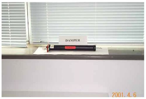

Figure 45. Drawing. Cross section of airpot damper.

The airpot damper uses the ambient air as the damping medium. The force to be damped is transmitted through the airpot piston rod, which moves the piston within the cylinder. The orifice setting and the diametric clearance between the piston and cylinder control the rate of air transfer. As the piston moves in response to the force exerted, there will be a change in volume and pressure in the airpot, causing ambient air to enter or leave the cylinder. The rate of airflow can be controlled to provide the exact degree of damping required by a simple adjustment of the orifice.

However, as the tests were prepared, it was found that the frictional damping between the piston and the cylinder wall inside the airpot damper had a significant impact on the small-amplitude motion, which suppressed the hand-excited cable vibration in just a few cycles. Finally, the airpot damper was only used in the cases of very high level damping with the order of 1 percent of critical, while for the intermediate- and high-level damping cases, elastic bands were used along the spring coils to increase the system damping (figure 46). By adjusting the number and locations of the elastic bands to be installed on the spring coils, the desired structural damping levels were achieved.

Figure 46. Photo. Elastic bands on the spring coils.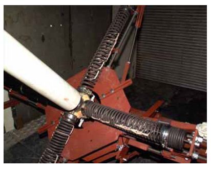

Surface Treatment

To explore the surface roughness effect on the cable oscillation, a kind of liquid glue was sprayed on the windward side of the model surface to simulate the accumulation of dirt and salt on the real cable.

Frequency Ratio

One distinguishing response characteristic of cable galloping is that the motion follows an elliptical trajectory. In the current model setup, the stiffness of the two pairs of perpendicular springs will affect the amplitude of motion in these two directions, and thus the resultant oscillation path of the cable. By properly adjusting the spring stiffness of these two directions, the associated in-plane and out-of-plane vibration frequencies are changed. If the frequencies are close enough, the motions in these two directions would become resonant, which form an elliptical shape of the motion path. Thus, the impact of the frequency ratio between the two perpendicular directions on the cable behavior of interest is worth studying.

Outline of Test Cases

The aerodynamic behavior of the inclined cable model has been investigated in this wind tunnel testing by different combinations of model setup, damping level, and surface roughness as described in Tables 11, 12, and 13, respectively.

Figures 47 through 49 show the model setups of the investigated cases in the wind tunnel tests, and figure 50 shows a picture of the inclined cable setup in the wind tunnel.

Figure 47. Drawing. Side view of setups 1B and 1C.

Figure 48. Drawing. Side view of setups 2A and 2C.

Figure 49. Drawing. Side view of setups 3A and 3C.

Figure 50. Photo. Cable setup in wind tunnel for testing.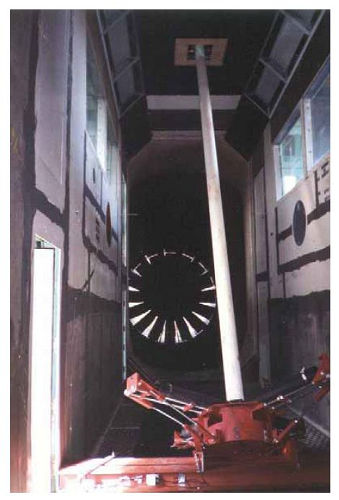

RESULTS AND DISCUSSION

General Procedures for a Given Test Setup

For a given case with its specific setup, the general procedures of the wind tunnel test are as follows:

• In still air, take tare case of the model.
• Measure the system structural damping in X- and Y-directions by hand exciting the model along these two directions respectively. Once the desired amplitude level is reached, stop the hand excitation and let the model undergo free vibration. The structural damping of the system and the vibration frequency can thus be identified.
• Start at the low wind speed (for the setup that is tested for the first time, take 7 m/s (23 ft/s), while for other cases, the starting value can be determined based on previous trials), increase in 2-m/s (6.5-ft/s) increments. When the wind speed approaches the expected unstable range, increase the speed by 1 m/s (3.3 ft/s) until unstable vibrations occur.
• In reality, some external effects such as wind turbulence and motions of the deck may help to initiate cable vibrations. Thus, during the tests, if no unstable vibration occurs within the expected wind speed range, hand excitation will be used to help initiate the unstable motion of the model and see if the motion decays or grows.
• If the unstable behavior is observed, add additional damping to the system. Repeat the above procedure for different damping levels until the unstable motion is eliminated.
• For the low damping level (no additional damping added), change the surface roughness and repeat the same procedure.

Characteristics of Cable Motion

Both the divergent type of cable vibration and the limited-amplitude cable motion at a certain wind speed range have been observed in the current study.

Divergent Type of Motion

Motions of the cable that resembled divergence were observed only in setup 2C. For this setup, the model has a vertical angle of Φ = 60°, and the spring rotation angle of α = 54.7°. This is equivalent to the full-scale cable orientation of the vertical inclination angle θ = 45° and horizontal yaw angle β = 45°.

The relationships between the system structural damping and response amplitude were obtained by hand exciting the model in X- and Y-directions, respectively. The maximum amplitude of the hand excitation was about 35 mm (1.4 inches). The free vibration immediately following the hand excitation was recorded for 15 minutes. The amplitude-dependent structural damping as a percentage of critical values in X- and Y-directions are given in figure 51. The vibration frequency in the X-direction is 1.400 Hz, and that in the Y-direction is 1.415 Hz.

The wind-induced response of setup 2C is given in figure 52. The test started at a low wind speed of 10 m/s (30 ft/s). When wind speed reached 32 m/s (105 ft/s), the motion became more organized and the amplitude in the Y-direction was built up steadily from ±20 to ±80 mm (±0.8 to ±3.1 inches) within 3 minutes. As shown by figures 53–57, which are the time histories in the X- and Y-motion at both ends of the model and the motion trajectory, the predominant motion occurs in the Y-direction. The motion had the tendency of growing further, but it had to be manually suppressed because of the clearance for the model setup at the wind tunnel ceiling. The recorded peak-to-peak amplitude was about 1D, where D is the cable diameter.

Limited-Amplitude Motion

The limited-amplitude unstable motion of the inclined cable model has been observed at certain wind speed levels under setups 2A, 1B, 1C, and 3A. The full-scale cable orientation angles, the model setup angles, and the unstable wind speed ranges corresponding to each individual case are given in table 14.

Figures 58–87 show the time histories at both ends of the model as well as the trajectory of the motion for those four different setups when unstable behavior of the cable was observed.

Three sets of time histories are given in figures 58–69 for setup 2A. The first and second set describe the time history and trajectory of the cable motion at wind speed of 18 m/s (59 ft/s) during the first and second 5 minutes, whereas the third set describes the time history and trajectory of the motion when wind speed increased to 19 m/s (62 ft/s). It can be clearly seen from these three sets that the vibration amplitude in the X-direction increases from about ±20 to about ±50 mm (±0.8 to ±2 inches) within the first 5 minutes of U = 18 m/s (59 ft/s), then increases a little bit to ±60 mm (±2.3 inches) and stays steadily at that level during the second 5 minutes of U = 18 m/s (59 ft/s). Once the wind speed increases to 19 m/s (62 ft/s), the vibration amplitude in the X-direction starts reducing slowly.

The relationship between the wind speed and response of these four setups are given in figures 88–91. The unstable ranges are clearly indicated by the peaks in the response curves.

Based on observations, this limited-amplitude cable motion looks more like vortex shedding excitation rather than galloping. The characteristics of the motion are summarized as follows:

• The amplitude of the motion is limited. As given in table 13, the largest amplitude observed is in setup 2A. When wind speed is 19 m/s (62 ft/s), the amplitude of the cable motion reaches 67 mm (2.6 inches).
• The vibration was observed only in the limited wind speed range at different wind speed levels. The reduced wind velocities corresponding to these ranges are approximately the multiples of 20.
• The maximum magnitude of the vibration depends on the orientation angle of the cable. It is larger with a greater vertical inclination angle, as given in table 14. In setup 3B, which represents the full-scale cable with a very shallow inclination angle of 20° and yaw angle of 29.4°, no unstable motion was observed within the wind speed range of 8–34 m/s (26–111.5 ft/s). Figure 92 gives the response of the cable with respect to wind speed in setup 3B. It can be seen that the amplitude of the motion stayed at less than 5 mm (0.2 inch).
• At the wind speed range where the cable motion was observed, there are two types of response: one is an organized harmonic motion, another is with a regular beating, which is similar to what Matsumoto described as the case of 3D Karman vortex shedding excitation.⁽¹⁶⁾ He explains that this regular beating is caused by the aerodynamic interaction between the axial vortices along the inclined cable surface and the ordinary Karman vortices in the wake of the cable. The Karman vortex shedding is amplified intermittently by the axially produced vortices and induces the beating type motion of the inclined cable.
• In some of the setups when the spring rotation angle is not 0°, which is equivalent to the wind horizontally oblique to the cable, an elliptical motion of the cable was observed, which correlates well with the field observation.⁽⁶⁾
• The critical Reynolds number at which the sudden decrease in the drag coefficient occurs is influenced both by surface roughness and flow turbulence. The critical Reynolds number range for a smooth circular cylinder under uniform flow is 2~4×10⁵, as shown in figure 93.⁽²⁸⁾ From the Reynolds numbers listed in table 13, it is interesting to observe that for the current study, all of these instabilities occurred more or less at wind speeds corresponding to this critical Reynolds number range.

Damping Effect

Four different levels of damping (i.e., low, intermediate, high, and very high damping) have been used in the tests to investigate the impact of structural damping on the aerodynamic behavior of the inclined cable.

A comprehensive set of damping tests was carried out with the model setup 1B, which represents the cable vertical inclination angle of 45° and horizontal yaw angle of 0° in full-scale bridge cables. No additional damper was applied for the low damping case. For the intermediate and high damping cases, the elastic bands were used to bind the spring coils together to increase the system damping, as shown previously in figure 46. The achieved damping level depends on the number and locations of the elastic bands. To obtain the intermediate level of damping, 16 elastic bands were used on each sway spring in the X-direction; while for the high damping level, 28 elastic bands were used on each spring in both X- and Y-directions. The very high damping level was achieved by installing the airpot dampers at both ends of the model with 1.25 dial turn.

The relationship between the critical damping ratio and the sway amplitude corresponding to these four levels of damping are given in figure 94. Figure 95 gives the wind-induced response of the cable model with setup 1B under those four levels of damping. As clearly shown in the figure, when the damping is increased, the response is significantly reduced, but the position of the unstable wind speed range does not change. This set of results indicates that this limitedamplitude unstable motion can be suppressed by increasing the damping of the cable.

Surface Roughness Effect

The cable model has been tested under both smooth and rough surface conditions. For the rough surface case, a kind of liquid glue was sprayed on the windward side of the model to simulate the accumulation of dirt and salt on the real cable.

Figures 96–98 describe the response of the model cable with setups 3A, 1B, and 2A under both smooth and rough surface conditions. These three cases are equivalent to wind blowing along the cable in full-scale situation. The vertical inclination angles θ are 35°, 45°, and 60°, respectively.

It can be seen from these three figures that for setups 3A and 1B, of which the inclination angle θ ≤ 45°, the increase of cable surface roughness makes the unstable response range shift to lower wind speed. For setup 2A, there are two peaks in the sway response curve of the smooth surface case: one is around 19 m/s (62 ft/s), and another is at about 34 m/s (111.5 ft/s). However, in the rough surface case, only one peak is identified, which is in the range of 31–32 m/s (101.7–105 ft/s). No clear peak shift phenomenon can be found for this setup. Since the inclination angles of these three setups are different, the difference in the responses given by those three figures not only include the surface roughness effect, but the influence of the orientation of the cable as well. Therefore, although the increase of cable surface roughness makes the unstable response range shift to lower wind speed for the cases of θ ≤ 45°, the conclusion regarding the surface roughness effect is still inconclusive from the present study alone.

The difference between the surface roughness would affect the flow separation point of the cable model, which changes the critical Reynolds number. This is likely to alter the lift and drag forces acting on the inclined cable, and thus changes its aerodynamic behavior. Further, a recent study shows that the change of orientation angle of the smooth cylinder will also affect the Reynolds number.⁽²⁹⁾ To better understand the mechanism of the unstable motion of the inclined cable and develop methods to eliminate or mitigate the instability, it is very important to further explore this Reynolds number effect.

Frequency Ratio Effect

In real cable-stayed bridges, the horizontal and vertical frequencies of the stay cables are slightly different. The design of the cable model and supporting rig in the current project faithfully reproduced this characteristic. Results obtained from the tested cases show that for the vibration of the cable model, the predominant motion was always in the direction of higher frequency. To investigate the impact of frequency ratio on the aerodynamic behavior of inclined dry cable, efforts were made to change the frequency ratio between the horizontal and vertical motions. Tests were conducted for three different frequency ratios with setup 2A:

• Case 1: ƒ_s = 1.477 Hz, ƒ_v = 1.452 Hz, ƒ_s/ƒ_v= 1.017.
• Case 2: ƒ_s = 1.460 Hz, ƒ_v = 1.448 Hz, ƒ_s/ƒ_v= 1.008.
• Case 3: ƒ_s = 1.428 Hz, ƒ_v = 1.432 Hz, ƒ_s/ƒ_v= 0.997.

where ƒ_s is the sway frequency in the X-direction, and ƒ_v is the vertical frequency in the Y-direction. All three cases were done with the smooth surface condition. For cases 1 and 2, 28 elastics bands were applied on each spring. In case 1, the elastic bands were placed such that they not only bound the spring coils into several groups, but touched the steel rods inside the spring coils as well. In case 2, only half number of the elastic bands touched the rods. To get higher frequency in the Y-direction in case 3, the elastic bands on the sway springs were removed, and those kept on the vertical springs did not touch the steel rod.

Figures 99–102 show the damping records and responses corresponding to these three cases. In figure 99, which is the damping of the motion in the X-direction, case 3 has a much lower damping ratio within the same amplitude range as compared with case 1 and 2. This is because in case 3, the elastic bands on the sway springs were removed, which reduced the system damping in the X-direction. The larger sway response of case 3 shown in figure 101 correlates well with this fact.

From the response curves shown in figures 101–102, no clear effect of the frequency ratio can be identified. This could be that the differences between the frequencies of those three cases are too small. Also, by using elastic bands to change the frequencies, the system damping was also affected. To further explore this frequency ratio effect, it will be a better approach to get different frequencies by adjusting the stiffness of the springs. Therefore, other effects, such as the change in the system damping, can be kept as small as possible.

Comparison with Other Studies

A limited number of experimental studies on inclined cables have been conducted, many of these in Japan. Saito et al. defined an instability criterion for the inclined cable motion based on three different model setups.⁽¹³⁾ Two of them are exactly the same as setup 1B and 2A in the current study. Miyata et al. investigated the inclined dry cable motion with one model setup, which corresponds to setup 2C in the present series of tests.⁽¹⁷⁾ To make comparison, these two sets of results, as well as the results obtained from the current study are shown together in figure 103. Among the results from current findings, only the one corresponding to setup 2C exhibited signs of divergent galloping motion, whereas the others are all high-speed vortex shedding excitation. The Scruton number is defined as Sc = mζ/ρD² , where m is cable mass per unit length, ζ is the logarithmic decrement, ρ is the air density, and D is the cable diameter. As can be seen from the figure, the boundary for instability defined by Saito et al.⁽¹³⁾ is much more conservative when compared with the results given by Miyata et al.⁽¹⁷⁾ and the current study. In addition, the similar instability criterion that could be defined by current findings would have much steeper slope than that given by Saito et al.⁽¹³⁾, which implies that with the increase of the cable structural damping, the instability range of the inclined cable motion will be shifted to even higher wind speed level, or the motion would be effectively eliminated.

Figure 51. Graph. Amplitude-dependent damping (A, sway; B, vertical) with setup 2C (smooth surface, low damping).

Figure 52. Graph. Divergent response of inclined dry cable (setup 2C; smooth surface, low damping).

Figure 53. Graph. Lower end X-motion, time history of setup 2C at U = 32 m/s (105 ft/s).

Figure 54. Graph. Top end X-motion, time history of setup 2C at U = 32 m/s (105 ft/s).

Figure 55. Graph. Lower end Y-motion, time history of setup 2C at U = 32 m/s (105 ft/s).

Figure 56. Graph. Top end Y-motion, time history of setup 2C at U = 32 m/s (105 ft/s).

Figure 57. Graph. Trajectory of setup 2C at U = 32 m/s (105 ft/s).

Figure 58. Graph. Lower end X-motion, time history of setup 2A at U = 18 m/s (59 ft/s) in the first 5 minutes.

Figure 59. Graph. Top end X-motion, time history of setup 2A at U = 18 m/s (59 ft/s) in the first 5 minutes.

Figure 60. Graph. Lower end Y-motion, time history of setup 2A at U = 18 m/s (59 ft/s) in the first 5 minutes.

Figure 61. Graph. Top end Y-motion, time history of setup 2A at U = 18 m/s (59 ft/s) in the first 5 minutes.

Figure 62. Graph. Lower end X-motion, time history of setup 2A at U = 18 m/s (59 ft/s) in second 5 minutes.

Figure 63. Graph. Top end X-motion, time history of setup 2A at U = 18 m/s (59 ft/s) in second 5 minutes.

Figure 64. Graph. Lower end Y-motion, time history of setup 2A at U = 18 m/s (59 ft/s) in second 5 minutes.

Figure 65. Graph. Top end Y-motion, time history of setup 2A at U = 18 m/s (59 ft/s) in second 5 minutes.

Figure 66. Graph. Lower end X-motion, time history of setup 2A at U = 19 m/s (62 ft/s).

Figure 67. Graph. Top end X-motion, time history of setup 2A at U = 19 m/s (62 ft/s).

Figure 68. Graph. Lower end Y-motion, time history of setup 2A at U = 19 m/s (62 ft/s).

Figure 69. Graph. Top end Y-motion, time history of setup 2A at U = 19 m/s (62 ft/s).

Figure 70. Graph. Lower end X-motion, time history of setup 1B at U = 24 m/s (79 ft/s).

Figure 71. Graph. Top end X-motion, time history of setup 1B at U = 24 m/s (79 ft/s).

Figure 72. Graph. Lower end Y-motion, time history of setup 1B at U = 24 m/s (79 ft/s).

Figure 73. Graph. Top end Y-motion, time history of setup 1B at U = 24 m/s (79 ft/s).

Figure 74. Graph. Lower end X-motion, time history of setup 1C at U = 36 m/s (118 ft/s).

Figure 75. Graph. Top end X-motion, time history of setup 1C at U = 36 m/s (118 ft/s).

Figure 76. Graph. Lower end Y-motion, time history of setup 1C at U = 36 m/s (118 ft/s).

Figure 77. Graph. Top end Y-motion, time history of setup 1C at U = 36 m/s (118 ft/s).

Figure 78. Lower end X-motion, time history of setup 3A at U = 22 m/s (72 ft/s).

Figure 79. Top end X-motion, time history of setup 3A at U = 22 m/s (72 ft/s).

Figure 80. Graph. Lower end Y-motion, time history of setup 3A at U = 22 m/s (72 ft/s).

Figure 81. Graph. Top end Y-motion, time history of setup 3A at U = 22 m/s (72 ft/s).

Figure 82. Graph. Trajectory of setup 2A at U = 18 m/s (59 ft/s), first 5 minutes.

Figure 83. Graph. Trajectory of setup 2A at U = 18 m/s (59 ft/s), first 5 minutes.

Figure 84. Graphic. Trajectory of setup 2A at U = 19 m/s (62 ft/s).

Figure 85. Graphic. Trajectory of setup 1B at U = 24 m/s (79 ft/s).

Figure 86. Graphic. Trajectory of setup 1C at U = 36 m/s (119 ft/s).

Figure 87. Graph. Trajectory of setup 3A at U = 22 m/s (72 ft/s).

Figure 88. Graph. Wind-induced response of inclined dry cable (setup 2A; smooth surface, low damping).

Figure 89. Graph. Wind-induced response of inclined dry cable (setup 1B; smooth surface, low damping).

Figure 90. Graph. Wind-induced response of inclined dry cable (setup 1C; smooth surface, low damping).

Figure 91. Graph. Wind-induced response of inclined dry cable (setup 3A; smooth surface, low damping).

Figure 92. Graph. Wind-induced response of inclined dry cable (setup 3B; smooth surface, low damping).

Figure 93. Graph. Critical Reynolds number of circular cylinder (from Scruton).⁽²⁷⁾

Figure 94. Graph. Damping trace of four different levels of damping (setup 1B; smooth surface).

Figure 95. Graph. Effect of structural damping on the wind response of inclined cable (setup 1B; smooth surface).

Figure 96. Graph. Surface roughness effect on wind-induced response of dry inclined cable (setup 3A; low damping).

Figure 97. Graph. Surface roughness effect on wind-induced response of dry inclined cable (setup 1B; low damping).

Figure 98. Graph. Surface roughness effect on wind-induced response of dry inclined cable (setup 2A; low damping).

Figure 99. Graph. Amplitude-dependent damping in the X-direction with setup 2A (frequency ratio effect).

Figure 100. Graph. Amplitude-dependent damping in the Y-direction with setup 2A .

Figure 101. Graph. Wind-induced response of inclined cable in the X-direction with setup 2A (frequency ratio effect).

Figure 102. Graph. Wind-induced response of inclined cable in the Y-direction with setup 2A (frequency ratio effect).

Figure 103. Graph. Comparison of wind velocity-damping relation of inclined dry cable.

Previous | Table of Contents | Next