• Federal Highway Administration >
• Publications >
• Research Publications >
• 05083 >
• Chap3.Cfm >
• Chapter 3. Analysis, Evaluation, and Testing

Previous | Table of Contents | Next

Chapter 3. Analysis, Evaluation, and Testing

MECHANICS OF WIND-INDUCED VIBRATIONS

There are a number of mechanisms that can potentially lead to vibrations of stay cables. Some of these types of excitation are more critical or probable than others, but all are listed here for completeness:

• Vortex excitation of an isolated cable or groups of cables.
• Rain/wind-induced vibrations of cables.
• Wake galloping of groups of cables.
• Galloping of single cables inclined to the wind.
• Galloping of cables with ice accumulations.
• Aerodynamic excitation of overall bridge modes of vibration involving cable motion.
• Motions caused by wind turbulence buffeting.
• Motions caused by fluctuating cable tensions.

All of these mechanisms are discussed in detail in appendix C. Vortex excitation, rain/wind, wake galloping of groups of cables, and galloping of single dry inclined cables all require careful consideration by the designer and are summarized later in this section.

The following parameters are relevant to these wind-induced vibrations.

Reynolds Number

A key parameter in the description of compressible fluid flow around objects (such as wind around stay cables) is the Reynolds number. The Reynolds number is a measure of the ratio of the inertial forces of wind to the viscous forces and is given by equation 1:⁽¹⁰⁾

(1)

Strouhal Number

The Strouhal number is a dimensionless parameter relevant to vortex excitation (equation 2):

(2)

The Strouhal number remains constant over extended ranges of wind velocity. For circular cross section cables in the Reynolds number range 1×10⁴ to 3×10⁵, S is about 0.2.

Scruton Number

The Scruton number is an important parameter when considering vortex excitation, rain/wind-induced vibrations, wake galloping, and dry inclined cable galloping (equation 3):

(3)

This relationship shows that increasing the mass density and damping of the cables increases the Scruton number. Most types of wind-induced oscillation tend to be mitigated by increasing the Scruton number.

Vortex Excitation of an Isolated Cable and Groups of Cables

Vortex excitation is probably the most classical type of wind-induced vibration. It is characterized by limited-amplitude vibrations at relatively low wind speeds. Vortex excitation of a single isolated cable is caused by the alternate shedding of vortices from the two sides of the cable when the wind is approximately perpendicular to the cable axis. The wind velocity at which the vortex excitation frequency matches the natural frequency (N_r) is found in equation 4 by using the Strouhal number S:

(4)

The amplitude of the cable oscillations is inversely proportional to the Scruton number S_c. Increasing the mass and damping of the cables increases the Scruton number and therefore reduces oscillation amplitudes.

Inherent cable damping ratios can range anywhere from 0.0005 to 0.01, and an accurate value is difficult to predict. The lower end of this range is typical of very long cable stays without any grout infill, while the upper end of this range is more typical of shorter cable stays with grouting and perhaps some external damping. A realistic estimate of inherent cable damping ratios on inservice bridges is in the range from 0.001 to 0.005. (See chapter 3 for field measurements.)

For example, a cable consisting of steel strands grouted inside the cable pipe and with a damping ratio (ζ) of 0.005 has a Scruton number of about 12, and the amplitude of oscillation is only about 0.5 of a percent of the cable diameter. During construction and before grouting, the damping ratio of stay cables can be extremely low (e.g., 0.001), and the amplitude could conceivably increase to about 4 percent of the cable diameter, which is still small. Therefore, vortex shedding from the cables is unlikely to be a major vibration problem for cable-stayed bridges. By adding a small amount of damping, vortex excitation will be suppressed effectively.

Rain/Wind-Induced Vibrations

The combination of rain and moderate wind speeds can cause high-amplitude cable vibrations at low frequencies. This phenomenon has been observed on many cable-stayed bridges and has been researched in detail.

Rain/wind-induced vibrations were first identified by Hikami and Shiraishi on the Meiko-Nishi cable-stayed bridge.⁽¹¹⁾ Since then, these vibrations have been observed on other cable-stayed bridges, including the Fred Hartman Bridge in Texas, the Sidney Lanier Bridge in Georgia, the Cochrane Bridge in Alabama, the Talmadge Memorial Bridge in Georgia, the Faroe Bridge in Denmark, the Aratsu Bridge in Japan, the Tempohzan Bridge in Japan, the Erasmus Bridge in Holland, and the Nanpu and Yangpu Bridges in China. These vibrations occurred typically when there was rain and moderate wind speeds (8–15 m/s (18–34 mi/h)) in the direction angled 20° to 60° to the cable plane, with the cable declined in the direction of the wind. The frequencies were low, typically less than 3 Hz. The peak amplitudes were very high, in the range of 0.25 to 1.0 m (10 inches to 3 ft), violent movements resulting in the clashing of adjacent cables observed in several cases.

Wind tunnel tests have shown that rivulets of water running down the upper and lower surfaces of the cable in rainy weather were the essential component of this aeroelastic instability.^(11,12) The water rivulets changed the effective shape of the cable and moved as the cable oscillated, causing cyclical changes in the aerodynamic forces which led to the wind feeding energy into oscillations. The wind direction causing the excitation was approximately 45° to the cable plane. The particular range of wind velocities that caused the oscillations appears to be that which maintained the upper rivulet within a critical zone on the upper surface of the cable.

Some of the rain/wind-induced vibrations that have been observed on cable-stayed bridges have occurred during construction when both the damping and mass of the cable system are likely to have been lower than in the completed state, resulting in a low Scruton number. For the Meiko-Nishi Bridge, the Scruton number was estimated at 1.7. The grouting of the cables adds both mass and damping, and often sleeves of visco-elastic material are added to the cable end regions, which further raises the damping. The available circumstantial evidence indicates that the rain/wind type of vibration primarily arises as a result of some cables having exceptionally low damping, down in the ζ = 0.001 range.

Since some bridges have been built without experiencing problems from rain/wind-induced vibration of cables, it appears probable that, in some cases, the level of damping naturally present is sufficient to avoid the problem. The rig test data of Saito et al., obtained using realistic cable mass and damping values, are useful in helping to define the boundary of instability for rain/wind oscillations.⁽¹³⁾ Based on their results it appears that rain wind oscillations can be reduced to a harmless level using the following criteria in equation 5 for the Scruton number:⁽¹⁾

(5)

This criterion can be used to specify the amount of damping that must be added to the cable to mitigate rain/wind-induced vibrations.

Since the rain/wind oscillations are due to the formation of rivulets on the cable surface, it is probable that the instability is sensitive to the surface roughness. Several researchers have tried using small protrusions on the cable surface to solve the problem. Flamand has used helical fillets 1.5 mm (0.06 inch) high on the cables of the Normandie Bridge.⁽⁸⁾ The technique has proven successful, with a minimal increase in drag coefficient. This type of cable surface treatment is becoming a popular design feature for new cable-stayed bridges, including the Leonard P. Zakim Bunker Hill Bridge (Massachusetts), U.S. Grant Bridge (Ohio), Greenville Bridge (Mississippi), William Natcher Bridge (Kentucky), Maysville-Aberdeen Bridge(Kentucky), and the Cape Girardeau Bridge (Missouri).

Wake Galloping for Groups of Cables

Wake galloping is the elliptical movement caused by variations in drag and across-wind forces for cables in the wake of other elements, such as towers or other cables. This occurs at high wind speeds and leads to large amplitude oscillations. These oscillations have been found to cause fatigue of the outer strands of bridge hangers at end clamps on suspension and arch bridges. Similar fatigue problems are a theoretical possibility on cable-stayed bridges, but to date none have been documented.

The Scruton number is an important parameter with regard to wake galloping effects. An approximate equation for the minimum wind velocity U_CRIT above which instability can be expected due to wake galloping effects has been proposed.^(1,14,15) It is given by equation 6:

(6)

For circular sections, the constant c has an approximate median value of 40. For cable-stayed bridges, this constant depends on the clear spacing between cables, and the following range of values based on the cable spacing is commonly used:

• c = 25 for closely spaced cables (2D to 6D spacing).
• c = 80 for normally spaced cables (generally 10D and higher).

Due to the level of uncertainty associated with practical applications, it is recommended that these values be applied conservatively, exercising engineering judgment.

The critical wind velocity may be low enough to occur commonly during the life of the bridge. Wake galloping therefore has the potential to cause serviceability problems. The equation for U_CRIT suggests several possibilities for mitigation. By increasing the Scruton number or natural frequency, the cables will be stable up to a higher wind velocity. However, increasing the frequency is far more effective in raising U_CRIT due to the square root manifestation of S_c in equation 6. The Scruton number increases with additional damping. The natural frequency may be increased by installing spacers or crossties along the cables to shorten the effective length of cable for the vibration mode of concern.

It should be noted that wake galloping is not a major design concern for normal, well-separated cable arrangements. For unusual cases, however, it is recommended that some attention be paid to the possibility of wake galloping.

Galloping of Dry Inclined Cables

Galloping of single dry inclined cables is a theoretical possibility. Results from one experimental study seem to suggest that this could be a concern for cable-stayed bridges.⁽¹³⁾ Theoretical formulations predict that this galloping may occur at high wind speeds with possible large-amplitude vibrations and that many existing cable-stayed bridges are susceptible, but there is no evidence of their occurrence in the field.

Single cables of circular cross section do not gallop when they are aligned normal to the wind. However, when the wind velocity has a component that is not normal to the cable axis, anninstability with the same characteristics as galloping has been observed. For a single inclined cable the wind acts on an elliptical cross section of cable. An ellipticity of 2.5, corresponding to an angle of inclination of the cable of approximately 25°, can occur in the outermost cables of long-span bridges. (Ellipticity is defined as the maximum width divided by the minimum width; for example, a circle has an ellipticity of 1.0.) There is the potential for galloping instability if the level of structural damping in these cables is very low.

Saito et al. conducted a series of wind tunnel experiments on a section of bridge cable mounted on a spring suspension system.⁽¹³⁾ Their data suggest an instability criterion given approximately by the following (this general relation was given in a different form in equation 6 for wake galloping, with c = 40):

(7)

This data was for cases where the angle between the cable axis and wind direction was 30° to 60°. The above criterion is a difficult condition to satisfy, particularly for the longer cables of cable-stayed bridges with a typical diameter of 150 to 200 mm (6 to 8 inches). Further experimental research was necessary to confirm the results of Saito et al. and to extend the range of conditions studied.⁽¹³⁾ All of their experiments used low levels of damping, so it was important to investigate whether galloping of an inclined cable is possible at damping ratios of 0.005 and higher.

Based on existing information, it was apparent that galloping of dry inclined cables presented the biggest concern and biggest unknown for wind-induced vibration mitigation. The project team therefore focused the wind tunnel test program on this subject, as described in chapter 3 of this report.

WIND TUNNEL TESTING OF DRY INCLINED CABLES

Introduction

From the information reported on the various types of cable vibrations due to wind loads, it was determined that galloping of dry inclined cables was the most critical issue requiring further experimental research. The wind tunnel data of Saito et al. showed evidence of dry inclined cable oscillations with some of the characteristics of galloping, and stability criteria were suggested in their paper.⁽¹³⁾ However, based on their criteria, many existing cable-stayed bridges would have shown more evidence of dry cable galloping than has actually been observed. To clarify the dry cable galloping phenomenon and evaluate the stability criteria proposed by Saito et al., the research team conducted a series of wind tunnel tests of a full-size 2D sectional model of an inclined cable in the propulsion wind tunnel at the Montreal Road campus of the National Research Council Canada Institute for Aerospace Research (NRC-IAR).⁽¹³⁾ A full description of the testing is included in appendix D.

The objectives of this study were to:

• Investigate the existence of dry inclined cable galloping.
• Clarify the mechanisms of this type of vibration.
• Determine the effects of the following parameter—wind speed, structural damping, surface roughness, and wind direction.
• Refine the stability criterion proposed by Saito et al.⁽¹³⁾

The following section summarizes the test program and its results.

Testing

The model was developed to be similar to that used in the test carried out by Saito et al.⁽¹³⁾ A 6.7-m (22-ft)-long cable consisted of an inner steel pipe covered with a smooth polyethylene (PE) tube with an outside diameter of 160 mm (6.3 inches). The effective mass per cable length was 60.8 kg/m (40.9 lb/ft). The end supports at the upwind end were maintained out of the wind flow above the wind tunnel, and at least 5.9 m (19.2 ft) of the 6.7-m (22-ft) length of the cable was directly exposed to the wind tunnel flow.

Testing was performed for various levels of structural damping, cable frequency ratios, and surface roughness, and at various angles of wind flow. The cable model orientation was changed against the mean wind flow direction for several configurations. The model was supported in the wind tunnel with the angles Φ and α being adjustable to represent different θ and β combinations. Figure 38 in appendix D shows the relationship of these angles to the cable and wind direction. Similar to the Japanese studies, θ and β represent the angle between the horizontal plane and the cable, and the yaw angle between the wind direction and the longitudinal bridge axis, respectively.⁽¹³⁾ The orientation of the 2-degree-of-freedom springs(perpendicular to the cable longitudinal axis) could be rotated about the cable axis through an angle α. Φ is the angle between the wind tunnel floor and the cable. The angle is only important when the vertical and horizontal frequencies of the cable are tuned to different frequencies. In the wind tunnel, this led to testing with an adjustable virtual ground plane. The relationship between the cable and the mean wind direction is represented by equations 8 and 9:

(8)

(9)

The aerodynamic behavior of the inclined cable model was investigated with different combinations of model setup, damping level, and surface roughness as described in tables 1, 2, and 3.

Results Summary

Limited-amplitude oscillations were observed under a variety of conditions. The limited-amplitude vibrations occurred within narrow wind speed ranges only, which is characteristic of vortex excitation of the high-speed type described by Matsumoto.⁽¹⁶⁾ For the typical cable diameters and wind speeds of concern on cable-stayed bridges, the Reynolds number (defined in chapter 3) is in the critical range where large changes in the airflow patterns around the cables occur for relatively small changes in Reynolds number. The excitation mechanism is thus likely to be linked with these changes. The maximum amplitude of the response depended on the orientation angle of the cable. For wind blowing along the cable, for cables with a vertical inclination angle θ~45°, the increase of surface roughness made the unstable range shift to lower wind speeds.

The results of this testing showed a deviation from the criteria described in the introduction. While significant oscillations of the cable occurred (double amplitudes up to 1D), it is not conclusive that this was dry inclined cable galloping. In fact, as indicated above they had similar characteristics to Matsumoto’s high-speed vortex excitation.⁽¹⁶⁾ Divergent oscillations only occurred for one test setup at very low damping, and the vibrations had to be suppressed since the setup only allowed for amplitudes of 1D. Large vibrations were only found at the lowest damping ratios (ζ < 0.001). Above a damping ratio of 0.003, no significant vibrations (>10 mm(0.4 inch)) were observed.

Figure 1 shows the results of this experiment as compared with the instability line determined by Saito et al.⁽¹³⁾ The graph presents reduced wind velocity (Ur) versus the Scruton number (equation 10):

(10)

The bold points indicate cable motions with amplitudes from ±10 mm (±0.4 inch) to ±80 mm (±3.1 inches). Note the test rig would not allow for motions greater than ±80 mm (±3.1 inches). However, only one test case reached this limit and is denoted by the triangular point. One point from Miyata et al. is also shown.⁽¹⁷⁾

Conditions with oscillations less than ±10 mm (±0.4 inch) are denoted with an open circle. Many of these points lie in the region denoted as unstable based on the instability line of Saito et al.⁽¹³⁾ It is suggested that this line can be redefined based on the dashed line denoted as the FHWA instability line.

Figure 1. Graph. Comparison of wind velocity-damping relation of inclined dry cable.

This testing suggests that if even a low amount of structural damping is provided (ζ > 0.003), then vortex shedding and inclined cable galloping vibrations are not significant. This damping corresponds to a Scruton number of approximately 3, which is less than the minimum of 10 established for suppression of rain/wind-induced vibrations (discussed in chapter 3). Therefore dry cable instability should be suppressed by default if enough damping is provided to mitigate rain/wind-induced vibrations. A complete report of the wind tunnel testing by the project team on dry inclined cables is given in appendix D.

A second phase of testing was conducted on a static model to verify the findings of the initial study, using the same orientations where the large amplitude oscillations occurred. Pressure taps were added to record aerodynamic force measurements. The objectives of this phase were to clarify the mechanism of dry inclined cable galloping and investigate the differences between galloping and high-speed vortex shedding. The test report was not available as of the production of this document.

OTHER EXCITATION MECHANISMS

Effects Due to Live Load

This study was carried out by the project team to assess the amount of vibration caused by live loading and determine if this movement is significant as compared with wind vibration. To address this problem a computer model of a real bridge was subjected to a moving train load, and the vibrations of an individual cable were analyzed. A moving train has a greater effect on cables than passing trucks or random traffic. The cable tensions, displacements, and anchorage rotations obtained from the dynamic time history analysis were compared with an analysis ignoring all dynamic effects as well as the results obtained from influence line calculations, which are normally carried out during design. A summary of this work is given in this section, and the complete report is included in appendix H.

A 3D computer model of the Rama 8 Bridge in Bangkok, Thailand, was created for this analysis. The bridge has a single tower and a 300-m (984-ft) main span. The third longest cable (M26), with an unstressed length of 299.1 m (981 ft), was studied to determine the effects of live loading.

A static live load analysis was first conducted as a baseline using a five-car transit train, neglecting the dynamic properties of the train. Influence line analyses were performed to determine the maximum and minimum effects due to live load. For dynamic analysis, the transit train was modeled as a mass on damped springs and moved across the bridge at a speed of 80km/h (50 mi/h), taking into account the dynamic interaction between the train and the structure. The tension in cable M26 is plotted in figure 2 to compare the dynamic effects with the static effect. Note that the increase in maximum cable tension due to dynamic effects is less than 10 percent.

Figure 2. Graph. Cable M26, tension versus time (transit train speed = 80 km/h (50 mi/h)).

The results of this study indicated the following:

• A stay cable which is discretized with 20 elements accurately predicts the free vibration characteristics of a stay cable.
• Once the cable is modeled as part of the real structure with the tower and the deck providing realistic end conditions, the cable frequencies only change slightly but the mode shapes become spatial rather than being purely in-plane or out of plane.
• The cable tensions, displacements, and end rotations are dominated by the "static" deformation response associated with the passing of the moving load. Subsequent dynamic oscillations are typically an order of magnitude smaller than the static maximum.
• It appears that the dynamic response of the cable, during the train passage and in the subsequent free vibration phase, is driven by the vibration of the bridge deck.

Deck-Stay Interaction Because of Wind

Measurements of both deck and stay movements were taken at the Fred Hartman Bridge during the passage of a storm. For this specific record, figures 3 and 4 show the time histories (first 5 minutes) and power spectral densities (PSD) of vertical deck acceleration at midspan and of the adjacent stay cable AS24, respectively. Cable AS24 has a length of 198 m (650 ft) and a natural frequency of approximately 0.59Hz. Figure 5 shows the wind speed at deck level.

Figure 3. Graph. Time history and power spectral density (PSD) of the first 2 Hz for deck at midspan (vertical direction).

Figure 4. Graph. Time history and power spectral density (PSD) of the first 2 Hz for cable at AS24 (in-plane direction) deck level wind speed.

Figure 5. Deck level wind speed.

Figures 3 and 4 show a dominant frequency of vibration at approximately 0.58 Hz. It is important to note that this frequency corresponds quite closely to the third symmetric vertical mode of the superstructure, and is also close to the first mode of the stay cable AS24. This is an interesting and important observation since the first-mode vibrations of a cable at this level of acceleration are generally associated with large displacements. In fact, by integrating the acceleration time history, the displacement amplitude (peak to peak) was estimated to be approximately 1 m (3 ft).

Furthermore, by observing the time histories, the significant vibrations are initially observed at the deck instead of the cable. This observation, as well as the similarity of modal frequencies, suggests that the deck is driving the cable to vibrate with large amplitude in its fundamental mode. Vortex-induced vibration of the deck is thought to be the driving mechanism for this motion. Further studies are continuing to identify additional occurrences of this behavior for corroboration, and to better understand the underlying mechanisms and their consequences. These findings are not complete at the time of production of this report.

This appears to be a rare event; very few occurrences of this nature have been identified.

STUDY OF MITIGATION METHODS

The development of recommended design approaches was based on previous and current research focusing on cable aerodynamics, dampers, and crossties. Theories on the behavior of linear and nonlinear dampers and crosstie systems were developed and compared with field measurements on the Fred Hartman Bridge, Leonard P. Zakim Bunker Hill Bridge, Sunshine Skyway Bridge, and Veterans Memorial Bridge. Basic findings are discussed below, and more detailed discussions are found in appendix F and in the technical papers listed in appendix E.

Linear and Nonlinear Dampers

To suppress the problematic vibrations of stay cables, dampers are often added to the stays near the anchorages (because of practical limitations of installation). Although the mechanisms that induce the observed vibrations may still not be completely understood, dampers have had relatively widespread use and their effectiveness has been demonstrated. However, criteria for damper design are not well established. Current recommendations for required damping levels to suppress rain/wind-induced vibrations were developed using relatively simplified wind tunnel models, and it is not clear whether these guidelines are adequate or appropriate for vibration suppression in the field.⁽¹⁾ In addition, it is important to note that vibrations can occur in more than one mode of the cable, and little has been done to address the question of required damping levels for each mode. The anticipated widespread application of dampers for cable vibration suppression justifies further research aimed at better understanding the resulting dynamic system and refinement of design guidelines. An example of a damper provided to a cable anchorage is shown in figure 6.

Figure 6. Photo. Damper at cable anchorage.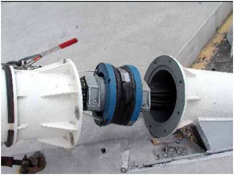

Linear Dampers

Free vibrations of a taut cable with an attached linear viscous damper were investigated in detail. In designing a damper for cable vibration suppression, it is necessary to determine the levels of supplemental damping provided in the first several modes of vibration for different values of the damper coefficient and different damper locations. Previous investigations of linear dampers have focused on vibrations in the first few modes for damper locations near the end of the cable. However, damper performance in the higher modes is of particular interest, as full-scale measurements indicate that vibrations of moderate amplitude can occur over a wide range of cable modes. This study investigates the dynamics of a taut cable damper system in higher modes and without restriction on the damper location (see figure 7).

Figure 7. Drawing. Taut cable with linear damper.

An analytical formulation of the complex eigenvalue problem for free vibration was used to derive an equation for the eigenvalues that is independent of the damper coefficient. This "phase equation" reveals the attainable modal damping ratios ζ_i and corresponding oscillation frequencies for a given damper location l /L, affording an improved understanding of the solution characteristics and revealing the important role of damper-induced frequency shifts in characterizing the response of the system. For damper locations, such as near the end of the stay, resulting in small frequency shifts, the following relationship can be derived in equations 11 and 12:

(11)

(12)

In figure 8, the normalized damping ratio ζ/(l /L) has been plotted against the nondimensional damping parameter,κ, for the first five modes for a damper location of l/L = 0.02, and it is evident that the five curves collapse very nearly onto a single curve in good agreement with the theoretical approximation.

Because the mode number is incorporated in the nondimensional damping parameter κ, the optimal damping ratio can be achieved in only one mode of vibration. This is a potential limitation for linear dampers because it is currently unclear how to specify, a priori, the mode in which optimal performance should be achieved for effective suppression of stay cable vibration, and designing a damper for optimal performance in a particular mode may potentially leave the cable susceptible to vibrations in other modes.

Figure 8. Graph. Normalized damping ratio versus normalized damper coefficient: Linear damper.

Nonlinear Dampers

The dynamic behavior of a taut cable with a passive, nonlinear, power law damper attached at an intermediate point was investigated. Recent studies indicated that a nonlinear damper may potentially overcome the limitation in performance of a linear damper whereby optimal damping performance can only be achieved in one mode of vibration.

The exact formulation of the complex eigenvalue problem for a taut cable with a linear damper was extended to develop a single-mode approximation for the amplitude-dependent effective damping ratios for the power law damper. An asymptotic approximate solution revealed a nondimensional grouping of parameters κ that was used to extend the universal estimation curve for the linear damper to the case of a nonlinear damper. For a damping exponent of β = 1 (linear damper), the expression for κ is the same as the previous equation derived for a linear damper. The shape of the curve is slightly different for each value of damping exponent, β, but for a given damping exponent the curve is nearly invariant with damper location and mode number over the same range of parameters as the universal estimation curve for the linear case (figure 9).

Figure 9. Graph. Normalized damping ratio versus normalized damper coefficient (β = 0.5).

Because the nondimensional damping parameter κ depends on both the amplitude and mode number of oscillation, the optimal damping performance will be achieved, in general, at different amplitudes of vibration in each mode. An "optimal" value for the damper coefficient can be determined by specifying a design amplitude of oscillation in a given mode at which the optimal performance is desired. Therefore, a nonlinear damper has the potential to allow optimal damping performance over a wider range of modes than would a linear damper.

In the special case of β = 0.5 (a square-root damper), it was observed that the damping performance is independent of mode number and depends only on the amplitude of vibration. In designing a square-root damper it is sufficient to specify only the amplitude, A_opt, and the optimal damping performance is achieved at the same amplitude in each mode. These features suggest that nonlinear dampers may offer some advantages over linear dampers for cable vibration suppression, while retaining the advantages of economy and reliability offered by a passive mitigation strategy.

Field Performance of Dampers

This investigation seeks to evaluate the effectiveness of passive linear dampers installed on two stays on a cable-stayed bridge by comparing response statistics before and after the damper installation and by investigating in detail the damper performance in a few selected records corresponding to different types of excitation.

Viscous dampers (dashpot type) were installed on two stays (A16 and A23) on the main span of the Fred Hartman Bridge (figure 10), a twin-deck, cable-stayed bridge over the Houston Ship Channel, with a central span of 380 m (1,250 ft) and side spans of 147 m (482 ft). The deck is composed of precast concrete slabs on steel girders with four lanes of traffic, carried by a total of 192 cables in four inclined planes, spaced at 15-m (50-ft) intervals.

Figure 10. Photo. Fred Hartman Bridge.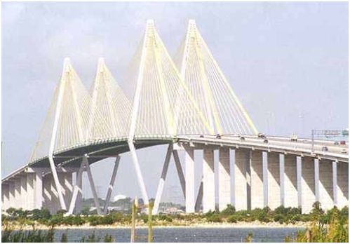

Properties of the two stays and the dampers that have been installed on these stays are given in table 4. Commercially available dampers were selected for the application.

Data have been collected for almost 3 years after the damper installation. The dampers were designed for optimal performance in the fundamental mode of vibration, which should provide adequate damping in the first several modes to suppress rain/wind-induced vibration. Wind speed is reported at deck level. Wind direction is measured in degrees clockwise from the bridge axis, with zero degrees corresponding to wind approximately from the north, directly along the bridge axis. Acceleration data are reported from transducers installed on the stays usually about 6 m (20 ft) vertically above deck level.

Results before damper installation show patterns that are consistent with other field and wind tunnel observations (see appendix F for additional details):

• A high density of points is seen near the abscissa, which generally corresponds to vortexinduced vibration in a variety of modes and low-level buffeting response of the stay to random excitations.
• Multiple points over a wide range of wind speeds are of high amplitude (RMS acceleration > 0.5 g), indicating the characteristic signature of rain/wind oscillation.
• One-minute mean wind speeds at deck level reached 15 m/s (34 mi/h) before the dampers were installed, and almost 18 m/s (40 mi/h) in the period after installation. This latter value corresponds to a 1-min average wind speed of 27 m/s (60 mi/h) at the top of the tower, recorded during a thunderstorm.
• The dependence on wind direction is also clear, with A16 showing its peak responses between 90° and 160°, and A23 over a narrower range between 90° and 135°.

Results after installation of the dampers suggest the following:

• Amplitudes are significantly reduced across all recorded wind speeds (up to 18 m/s (40 mi/h) at deck level) with maximum RMS acceleration amplitudes of around 0.5 g.
• The dependence on wind direction has been altered significantly, the largest responses now nearer to a 90° angle of incidence.
• Based on the measured forces in the dampers, they are functioning and providing dissipative force to the stays as intended.

In conclusion, the benefits of adding dampers are evident. Dampers can potentially be attached unobtrusively near the stay anchorage at the deck or tower, and thus detract minimally from the aesthetics of the structure.

Crosstie Systems

One possible method to counteract undesired oscillations is to increase the in-plane stiffness of stays by connecting them together with a set of transverse secondary cables, defined as crossties. From a dynamic perspective, the properties of the single cables are modified by the presence of the lateral constraints that influence their oscillation characteristics. Similarly, a connection of simple suspended elements is transformed into a more complex cable network. Figure 11 shows an example of cable crosstie systems applied to a bridge.

Figure 11. Photo. Cable crosstie system.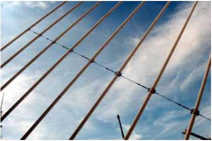

Detailed studies of crossties and interconnected cable systems are not well reported, and most of the recommendations that are currently followed seem to be linked to practice or previous experience. A fundamental study to better understand the behavior was therefore necessary.

Such study has shown that crossties potentially work by increasing the generalized mass and therefore Scruton number in the lower modes, and by raising frequencies and localizing the vibration in higher modes. They are also likely to increase the effective damping of a cable through the friction at crosstie connections and by providing a mechanism to transfer energy from one cable to another. However, these statements are difficult to quantify reliably using analytical methods.

The Dames Point Bridge (figure 12) in Jacksonville, FL, is an example of the effective use of crossties on an older bridge designed before the discovery of rain/wind-induced vibrations. Although some wind-induced oscillations were observed during construction before grouting and crosstie installation, no problematic cable vibrations have been reported on this bridge since it was completed in 1989.

Figure 12. Photo. Dames Point Bridge.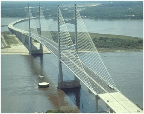

There is also the potential to combine cable crossties and dampers into a single device.⁽¹⁸⁾ This could provide an efficient system where a damper at one location provides damping to a system of cables through the crossties. The method could be highly effective as the damping would be provided at a point significantly into the cable length, but issues of aesthetics and serviceability need to be further addressed.

Analysis

An alternative analytical method was developed to examine cable crosstie networks and was used to study the Fred Hartman Bridge cable system.

Limited study of in-plane vibrations of complex cable networks has usually been performed by means of finite element methods because of the number of cable elements that are involved and the variability of the global characteristics of the system. An analytical method and efficient numerical procedure was developed that models the behavior of a set of interconnected cables. The analytical method is an alternative procedure for the derivation of the equation of motion (free-vibration problem) of a network, based on the taut cable theory. This approach offers a number of advantages over the finite element method and provides a tool that is useful in the design and optimization of such systems for practical application.

The initial problem formulation is depicted in figure 13. The example shows a simplified network, defined by a set of two taut cables connected by means of a vertical rigid rod (to be relaxed later). (See appendix F for the formulation of the analytical method for this system.)

Figure 13. Chart. General problem formulation.

The free-vibration analysis method was applied to the study of a cable network that was modeled after the Fred Hartman Bridge. The investigated system corresponds to the south-tower centralspan portion, a set of 12 stays with a three-dimensional arrangement (figure 14). Stay 24S is

Figure 14. Chart. General problem formulation (original configuration).

assumed as a reference element; all other stay quantities are normalized with respect to this element. The transverse connectors, an "eight-loop" steel wire rope system, are located in accordance with the existing system. The three-dimensional cable network was reduced to an equivalent two-dimensional problem. The definition of the modal frequencies and mode shapes of the network (free-vibration analysis) was performed through the study of the roots of the determinant of the system matrix as a function of the reduced frequency of the structure.

Figures 15 and 16 depict the eigenfunctions for modes 1 and 5 of the model, normalized so that the resulting modal mass of the network is unitary. A careful study of the solution patterns showed two categories of roots:

• Global modes, where the whole set of cables is involved in the oscillation (e.g., mode 1).
• Local modes, where the maximum amplitudes are located in the intermediate segments of specific cables. The overall characteristics of these modal forms can be different from the solution for individual cables, and influenced by the presence and the location of the transverse connectors. The wavelength of these modes is essentially governed by the distance between two consecutive connectors (e.g., mode 5).

Figure 15. Graph. Eigenfunctions of the network equivalent to Fred Hartman Bridge: Mode 1.

Figure 16. Graph. Eigenfunctions of the network equivalent to Fred Hartman Bridge: Mode 5.

In figure 17, the natural frequencies (Hz) are plotted as a function of the mode number and compared with the individual cable behavior. Solutions are shown for three comparative cases (NET_3C, original configuration; NET_3RC perfectly rigid transverse links; NET_3CG modified nonrigid configuration with ground restrainers). For practical purposes, the connectors in the original configuration can be considered as effectively rigid since the two graphics (NET_3C, NET_3RC) essentially overlap.

From figure 17, it can be seen that the sequence of fundamental global modes is followed by a high-density solution pattern, corresponding to the localized modes. An upper and lower limit frequency can be detected, in this case 1.9 and 2.7 Hz, respectively. Both limits are connected by the frequency of antisymmetric second modes in the individual stays. The upper value is directly related to the frequency of shorter cables, while the lower value is influenced by a combination of the stays in the central part of the structure (presence of pseudosymmetric components). Thehigh density of frequencies suggests a potential sensitivity to forced oscillations, exciting the network within this range, in which the dynamics can be influenced by a combination of these modal forms. Beyond this upper limit the situation reverts to a set of higher network modes and thereafter, a second plateau appears in the frequency range coincident with high-order antisymmetric individual segment modes. This pattern of consecutive "steps" defines a typical pattern for the behavior.

Figure 17. Graph. Comparative analysis of network vibration characteristics and individual cable behavior: Fred Hartman Bridge.

Field Performance

Field measurements of the Fred Hartman Bridge were compared with analysis results to validate the analysis approach for crosstied systems. A long-term ambient vibration survey was conducted to monitor stay cable vibration and to better understand the overall performance of the structure and its modal characteristics. More than 10,000 trigger files were recorded during a period of 3 years and continued thereafter. An algorithm was designed for the automatic processing of the records.

The methodology was applied to the study of the side-span unit of the south tower of the bridge (see figure 18). The cable network is configured by means of three transverse restrainers. The data set was extracted from the records of four in-plane and out-of-plane accelerometers, placed along stays AS1, AS3, AS5, and AS9 at a height of approximately 7 m (22 ft) from the deck level. The correspondence between the predicted modal characteristics and the real behavior was carried out by simultaneous spectral analysis of the in-plane acceleration record database of the four locations. The analysis was founded on the simultaneous identification of the same dominant in-plane frequency on all the four investigated cables.

Figure 18. Chart. Fred Hartman Bridge, field performance testing arrangement.

The investigation considered the presence of cable network behavior along with individual cable and, eventually, global (deck) structure modes. The fundamental frequencies of each stay were identified through field measurements and were adopted as input data in the numerical procedure to allow for a consistent comparison of the results with the real situation. The results of the simulation are summarized in table 5, in which the frequencies of the modes between 0 and 4 Hz are indicated. The subdivision into global and local network modes is indicated along with information about the general characteristics of the modal shape.

The computed frequency of NM1 (0.926 Hz) is close to the 10^th bending mode of the bridge (0.924 Hz), which suggests a potential susceptibility to interaction of the deck-stay system in this range. Low-density values of frequency can be seen up to 2.4 Hz (NM5) and beyond 3 Hz (NM30). The plateau behavior was detected between 2.4 and 3.0 Hz, associated with local behavior and a high density of solutions (NM5–NM29).

The results of the field data analysis showed consistent similarities with the predicted values. They also indicated the potential presence of some of the "new" modal forms in frequency ranges in which modal characteristics from other sources (individual stays, global structure, etc.) were often excluded. NM1 was clearly identified in one occasion only for a continuous time interval of about 15 min, corresponding to an extremely rare occurrence in terms of ambient-induced vibration. This event was mainly driven by the high-amplitude motion of the deck due to vortex shedding and related to a strong wind with direction almost perpendicular to the bridge axis.

Considerations for Crosstie Systems

This analysis shows that careful consideration must be given to the design of crossties. The general frequency increment in the fundamental modes that is usually attained by the introduction of transverse connectors must be balanced with the potential undesirable behavior of the local modes. A set of considerations for the improvement of the response of a cable network is proposed:

• Keep the location of the first plateau as high as possible, distant from the fundamental modes, so that the antisymmetric individual cable modes (2^nd mode) that mostly contribute to the network modal shape are those of the shorter cables. Symmetric configurations of the restrainers with respect to intermediate-length cables is preferred to increase the frequency interval (lower limit in particular) corresponding to local modes since they minimize the longest segment length.
• Relative stiffness of the transverse restrainers does not seem to play a significant role in the definition of the modal characteristics. Rather, the frequency ratio among different stays (related to the reference cable frequency) seems to be responsible for the network mode sequence. A good compromise between small frequency ratios (shorter stays) and high values (longer stays) is preferred for the optimization of the system. Unfortunately, this aspect is not connected to the crosstied configuration but to the existing setup of the bridge.
• A cable network cannot be designed to withstand all possible excitations; the best thing that can be done is to select some sources of vibrations and "tune" the network not to respond to them since the behavior becomes complex because of the presence of the plateau. Localizedmodes are practically unmanageable since they mainly concern internal elements of thsystem, although in these cases the vibration is confined to a selected portion of the structure and the potential implications for long-term structural sensitivity (fatigue damage) are less relevant.
• A network, combined with additional mechanical dampers, connected to the deck at specific locations might be seen as an efficient way of vibration reduction. The presence of pseudosymmetric behavior should be carefully assessed: it generates "nondampable" modes (half of the structure is at rest). This behavior is enhanced by the presence of ground connectors. It might be possible to use a ground restrainer in the proximity of the shortest cable, close to the tower in combination with dampers on the segments on the right side of the longest cables closest to the deck. In fact, the first pseudosymmetric modes (in this model) are those related to the unconstrained regions of the network, and the presence of adamper in this position might become efficient. Such an opportunity must be balanced with the fact that, when the addition of these devices is necessary, the high inclination of the shortcables might make them difficult to install.
• Crossties may be less effective at controlling out-of-plane oscillations. This further suggests the importance of using dampers in coordination with crosstie systems.
• Finally, the optimal design of a network should be based not only on structural performance considerations but also on cost provisions (e.g., installation, maintenance). In this way, the preferred solution should be suggested perhaps through a more extended optimization technique.

Cable Surface Treatment

The effectiveness of different surface modifications is determined from wind tunnel tests. No accepted methodology exists for the design of these elements. All major cable suppliers provide cable pipes that include surface modifications to mitigate rain/wind-induced vibrations. Several types of cable surface treatments are shown in figure 19. Extensive research has been done in the past, and these surface treatments have been shown to be effective for mitigation of rain/windinduced vibration.

Figure 19. Drawing. Types of cable surface treatments.

The double-helix spiral bead formations are the most common on new bridges, such as the Leonard P. Zakim Bunker Hill Bridge (Massachusetts), U.S. Grant Bridge (Ohio), Greenville Bridge (Mississippi), William Natcher Bridge (Kentucky), Maysville-Aberdeen Bridge (Kentucky), and Cape Girardeau Bridge (Missouri). As a manufacturer proprietary item, test data demonstrating their effectiveness is generally available from the cable suppliers (figure 20).

Figure 20. Graph. Example of test data for spiral bead cable surface treatment.

FIELD MEASUREMENTS OF STAY CABLE DAMPING

Leonard P. Zakim Bunker Hill Bridge (over Charles River in Boston, MA)

FHWA performed measurements during construction of the Leonard P. Zakim Bunker Hill Bridge (figure 21), a cable-stayed bridge with inverted Y-shaped towers and a main span of 227 m (745 ft). The bridge is 56 m (183 ft) wide with 10 lanes (two cantilevered lanes). The cables are ungrouted and arranged in a single plane for the back spans and two inclined planes for the main span. External visco-elastic dampers at the roadway level, cable crossties, and a double helical fillet cable surface treatment were applied to mitigate cable vibrations. Measurements were taken before and after installation of dampers and crossties.

Figure 21. Photo. Leonard P. Zakim Bunker Hill Bridge.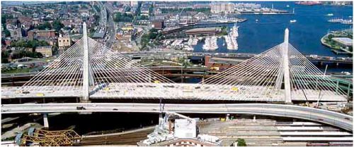

Preliminary results available as of this writing (private communication—reported data has not been independently verified by the study team) demonstrate the effectiveness of these mitigation methods. Table 6 shows the fundamental frequencies and damping ratios for the longest cables of the bridge before and after damper installation. In general, results show that the addition of dampers increases the frequency (by about 10 percent) and significantly increases the damping of the cables. Further evaluation of the measurements may be necessary, particularly since the data indicate that a few cables have smaller damping ratios after addition of dampers. In general, the damping ratio of ungrouted cables without external dampers appear to vary from 0.10 to 0.36 percent, with an average of 0.20 percent. The external dampers raise the cable damping to an average of 0.37 percent.

Figures 22, 23, and 24 show the time histories of decay of manually excited cables before installation of dampers and crossties, after damper installation, and after crosstie installation, respectively. The preliminary results demonstrate the effectiveness of not only the dampers, but also the cable crossties in raising the level of effective damping of the cable system. As the test method consisted of exciting one cable and recording the decay of its oscillations, some energy transferred from the excited cable to the adjoining cables through the crossties. Thus the reported damping with crossties may reflect values higher than the actual damping in the global system.

Figure 22. Graph. Sample decay: No damping and no crossties.

Figure 23. Graph. Sample decay: With damping and no crossties.

Figure 24. Graph. Sample decay: With damping and crossties.

Sunshine Skyway Bridge (St. Petersburg, FL)

The Sunshine Skyway Bridge (figure 25) has been in service since 1982 and has not had reported problems with cable vibrations. The bridge has a main span of 366 m (1,200 ft) between two single-mast towers and 84 cables in a single cable plane. The cables are provided with external viscous dampers (figure 26), but no crossties or surface treatment.

Figure 25. Photo. Sunshine Skyway Bridge.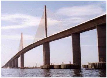

Figure 26. Photo. Stay and damper brace configuration.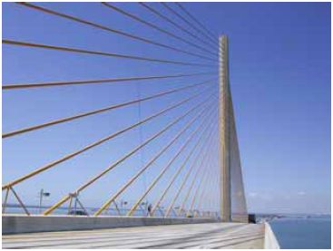

Field measurements on the cables of the Sunshine Skyway Bridge were taken to study damping in multiple modes of vibration. This data provides a baseline for comparison of future measurements to evaluate cable damping performance of other cable-stayed bridges. Table 7 contains preliminary frequency and damping estimates from the ambient data (private communication).

What also makes this set of data interesting is that the cables on the Sunshine Skyway Bridge are all installed with two inclined struts that are each connected to three viscous dampers. This type of configuration enables the dampers to provide supplemental damping in two directions, unlike the case of the dampers on the Fred Hartman Bridge, which are oriented in the in-plane direction only. In fact, no excessive cable vibrations have been reported for the Sunshine Skyway Bridge, even though it is located in a region full of frequent wind and rain, while for the cables of the Fred Hartman Bridge there were still cases of some reported large-amplitude vibrations in the lateral direction that could not be suppressed by the damper.

BRIDGE USER TOLERANCE LIMITS ON STAY CABLE VIBRATION

Field records from the large amplitude cable vibrations typical of rain/wind-induced vibration episodes have noted that such vibrations can have the effect of alarming bridge users and general observers on the safety of the structure. In reality, however, even for extreme cases, such vibrations have only produced limited damage to nonstructural cable anchorage components. In closer examination, even these failures of the secondary elements can generally be traced to fatigue prone or other unsuitable details. There is little field evidence to indicate permanent structural damage to the cables or other primary load carrying members as a result of rain/windinduced vibrations on the affected bridges. A detailed examination of the level of stress generated in the primary elements caused by these oscillations may generally indicate that the amplitude of dynamic stresses are not high enough to be a serious fatigue issue for cable strands or other bridge components either.

While the design displacements based on fatigue (or other design criteria) can be readily obtained through proper engineering calculations, there is little information in the literature to determine what level of cable oscillations can be permitted based on user tolerance to such displacements. In some cases, it can be expected that the displacement limits based on user acceptance may govern over those based on direct stress evaluation. The user acceptability threshold for a rural high-level crossing where the observer is the motorist could be much less critical than that for an urban bridge where the public may be able to observe the bridge in close proximity. Detailed determinations of such limits are both complex and somewhat subjective. Thus, at least a preliminary identification of these human comfort thresholds was deemed important in developing design guidelines.

A design criteria set forth by these factors would be independent of those required by the structural effects involved, similar in nature to existing codes limiting deflection in bridges or drift in tall buildings. The human mechanism of perception of stay cable vibration is quite different from, say, the perception of building or floor movement by an occupant. The former is purely visual, whereas the latter is mostly physical feel. If a building occupant is near a window, some visual aspects of building movement with respect to fixed features of the landscape may become apparent. However, buildings rarely may exhibit such levels of movement and it is likely that other design criteria may prohibit a building design this flexible. Building occupant comfort is typically ensured by limiting acceleration and jerk (rate of change of acceleration). For torsional movements of tall buildings, however, there are some limits based on visual perception that may have some level of similarity to the case under study. The parameters may be:

• User proximity (rural versus urban setting).
• Cable diameter.
• Cable displacement.
• Mode shape.
• Cable length.
• Velocity.

Focusing on typical cable sizes and typical vibration frequencies applicable to practical situations can further condense these parameters.

The study of user tolerance limits described in appendix I was an attempt to establish some preliminary criteria on user perception of stay cable vibrations. In this study, user perception was determined with vibration mode shape, velocity, and vibration amplitude as variables.

The two most important factors affecting user comfort were found to be the amplitude of the vibration and the velocity. As the frequency range is somewhat limited, it would stand to reason that the comfort criteria could be based on the amplitude. The study indicated that a reasonable recommendation of a limit on vibration amplitude (single) would be 1 cable diameter. Ideally, further reducing this to 0.5 diameters or below has the effect of making the vibrations virtually unnoticeable.

This study is preliminary and based on a relatively small sample size. Therefore, further investigation should be performed to refine any design criteria based on user comfort.

Previous | Table of Contents | Next