• Federal Highway Administration >
• Publications >
• Research Publications >
• Hydraulics Publications >
• 03052 >
• 05c.Cfm >
• Field Observations and Evaluations of Streambed Scour At Bridges

Field Observations and Evaluations of Streambed Scour At Bridges

CHAPTER 5: LOCAL SCOUR AT PIERS, continued

Table 7. Summary of weighted and unweighted regression results using basic variables.

Figure 14. Box plot illustrating the effect of pier shape on relative depth of scour.

Figure 15. Box plot illustrating the effect of pier shape on the depth of scour with the effects of pier width, velocity, depth, and bed material removed by linear regression.

Relative Velocity

Through a series of laboratory experiments, Chiew found relative scour depths (y_s/b) were less for ripple-forming sediments than for nonripple-forming sediments at relative velocities (V_o/V_c) ranging from 0.6 to 2.⁽⁴⁴⁾ He determined that this reduction in scour depth was caused by the roughness and sediment transport associated with the formation of ripples near incipient motion. Ripple-forming sediments are those with a D₅₀ less than about 0.6 mm. Figure 16 shows that the upper envelope of the field data generally fits the curves that Chiew developed.⁽⁴⁴⁾ A few measurements with ripple‑forming sediments exceed the envelope. The maximum depth of scour observed in the field does not appear to be strongly affected by whether the sediment is ripple forming or nonripple forming. The scatter of data below the envelope curves indicates that the relation between relative depth of scour and relative velocity developed in the laboratory does not adequately explain the scour processes in the field. Nonuniformity of the bed material and variable flow depth in the field probably cause some of the scatter.

Baker also did laboratory investigations of the effect of bed material properties on the relation between relative scour depths and relative velocity, using nonuniform bed material characterized by the coefficient of gradation.⁽⁴⁵⁾He found that as the coefficient of gradation increased, the relative depth of scour was reduced, and the maximum scour occurred at a relative velocity greater than one. The field data categorized by the coefficient of gradation are shown in figure 17 with hand-drawn envelope curves for the four categories of gradation. The effect of gradation has no consistent pattern in the relation between normalized scour depth and relative velocity for the field observations.

Baker changed the gradation while maintaining a constant D₅₀ during his experiments.⁽⁴⁵⁾ To simulate a constant D₅₀ in the field data, Mueller used partial residuals to remove the effect of D₅₀from the field data.⁽⁵⁾ This approach did not improve the comparison between the field data and Baker's laboratory observations.⁽⁴⁵⁾

Figure 17. Effect of gradation and relative velocity on relative depth of scour for field data, with hand-drawn envelope curves for selected gradation classes.

Bed Material Parameters

The scale of laboratory experiments prevents the effect of relative sediment size (b/D₅₀) on relative scour depth from being directly compared with field conditions. The maximum relative sediment size obtained in the laboratory was about 800. In the laboratory, ripple-forming sediments had lower relative scour depths than nonripple-forming sediments for relative sediment sizes ranging from 100 to 800. The field data do not contain ripple-forming sediments with a relative sediment size less than 900 (figure 18); therefore, there is insufficient overlap between laboratory and field data to make a valid comparison. The field data show a cluster of ripple-forming sediments near a relative sediment size of 1,000 that is below the maximum scour for nonripple-forming sediments; however, the maximum relative depth of scour for ripple-forming sediments with relative sediment sizes of 4,000 exceeds the nonripple-forming sediments.

Figure 18. Effect of relative sediment size on relative depth of scour for field data.

Figure 19. Effect of the coefficient of gradation on relative depth of scour for field data with hand-drawn envelope curves of ripple- and nonripple-forming sediments.

Depth of Approach Flow

Most researchers agree that for constant velocity intensity, local pier scour increases as depth of flow increases, but as the depth of flow continues to increase, the scour depth becomes almost independent of flow depth. (See references 44, 47, 69, 73, 74, 75, and 76.) Chiew⁽⁴⁴⁾ plotted data that he collected along with experimental data from Shen et al.,⁽⁹⁾ Ettema,⁽⁴⁷⁾ and Chee⁽⁷⁶⁾ and concluded that the flow depth does not affect scour if the depth is greater than four times the pier width. From this research, Melville and Sutherland developed the K_y factor in their prediction equation (table 3).⁽²⁾ The relation between relative flow depth and relative scour depth for the field data is shown in figure 20. Although the curve for the K_y factor envelops the data to the right, the data do not follow the trend of the curve. Most laboratory data are collected at or near incipient motion. To better compare the field data with the laboratory data, field data with sediment transport conditions near incipient motion (0.8 < V_o/V_c <1.2) were selected and plotted in figure 21. Again, the field data do not follow the trend observed in the laboratory data; they indicate that the relative depth of scour tends to increase with increasing relative flow depth.

DEVELOPMENT OF SCOUR PREDICTION METHODOLOGY

Assessment of Basic Variables

Logically, pier width, pier shape, flow depth, approach velocity, and bed material characteristics are important variables in determining the depth of scour; however, most of the design equations presented in table 3 do not contain all of these variables. The Mississippi equation, which was one of the top equations (table 5), is based on only pier width and flow depth. Therefore, it is important to evaluate the significance of each variable on the depth of scour and the potential interaction among the variables. A combination of scatter plots and multiple regression analysis will be used for this evaluation.

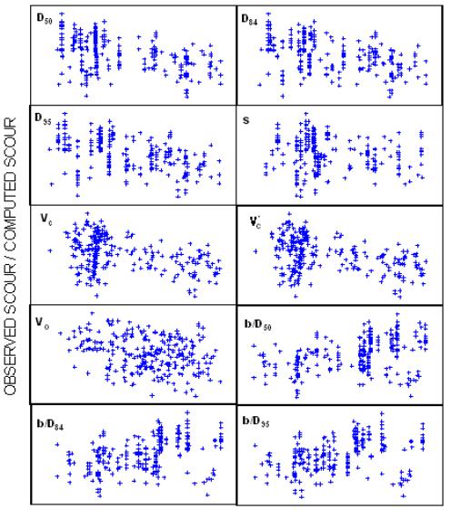
The effect of an individual variable on the depth of scour in the field is complicated by the interactive response of the variables to the dynamic conditions. Evaluating the effect of a particular variable on the depth of scour in the laboratory is easier than in the field. In the laboratory, all variables can be held constant and one variable changed; in the field, all of the variables interact and adjust to the changing flow conditions.

Figure 22 shows a scatterplot matrix of basic variables reported in the field data with a linear least squares smooth through the data. Drainage area, slope, and pier width appear strongly correlated with scour depth. Pier width directly affects the strength of the vortex system, which erodes the material from around the base of the pier. Correspondingly, pier width shows the strongest correlation with scour depth. It is surprising that drainage area and slope have a stronger correlation with the scour depth than do approach depth or approach velocity. This strong correlation appears to be caused by the correlation of the pier width and approach depth with drainage area and slope (figure 22); thus, for these data, drainage area or slope may represent a combined effect of pier width and approach depth. There is also a positive correlation between depth of scour, approach depth, and approach velocity; however there is significant scatter in the data, indicating that these variables are less significant than pier width. The size and distribution of the bed material also affects the depth of scour, but the slope of the linear smooth is small and the scatter of the data indicates a low correlation with the depth of scour. The bed material size is well correlated with the approach velocity and slope, which is what would be expected; coarse bed streams have higher slopes and higher velocities. The bed material size classes are strongly correlated with each other, but are not linearly correlated with the gradation coefficient. The strong linear correlation between bed material sizes could cause colinearity problems in the results of multiple linear regression if different bed material size variables are included in the same equation.

Weighted multiple linear regression analysis was used to assess the importance of each variable on the depth of scour, while accounting for the interaction between variables. Bed material sizes were evaluated in separate equations because of their strong colinearity. All variables were transformed logarithmically to improve the linearity and distribution of the data. Weighted multiple linear regression computes coefficients and exponents that minimize the sum of squares of the residuals while taking into account weights assigned to each observation. If the weights for all observations are equal, approximately one-half of the data are underestimated and about one-half are overestimated (figure 23). This approach, while yielding a combination of variables that fits the middle of the data, is not appropriate for design. An envelope curve is more appropriate for design. To fit an envelope curve, the regression was completed with equal weights, then the weights were adjusted so that more weight was applied to those points that were underestimated and defined the upper boundary of the data (figure 23). The weighting function (w), shown in equations 38 and 39, was determined by trial and error to produce a reasonable envelope curve.

Figure 23. Example of difference between unweighted regression and weighted regression in developing a design curve.

for residuals > 0

(38)

for residuals < 0

(39)

It was observed that small adjustments in the weighting function significantly change the sum of squared errors, the number of observations underestimated, and the statistical significance of each of the variables in the equation formulation. Therefore, the equations developed from this weighted regression approach should not be treated as the optimal envelope equation for these data, but serve as indicators as to which variables should be considered in the development of design methodology.

Regression analysis showed that the inclusion of bed material size characteristics in the equation improved the sum of squared errors (table 7). Unweighted regression indicated that only the bed material size was important and the gradation of the bed material was not statistically significant at the 0.1 level. The equation using the D₈₄ sediment size resulted in the lowest sum of squared errors. It is surprising that when the bed material was removed from the equation the approach velocity was not statistically significant in the unweighted regression. It is also interesting that there is reasonable consistency in the exponents for pier width and approach depth, but the exponents on velocity vary by a factor of 10.

The weighted regression analysis produced different results than did the unweighted analysis. As with the unweighted regression, the equations containing bed material characteristics all produced lower sum of squared errors than did the equations without bed material characteristics. For the weighted analysis, all of the variables in each analysis were significant, and the equation using D₅₀ produced the lowest sum of squared errors. While these equations may not be the optimal approach to predicting the depth of scour, they clearly show that bed material characteristics are important in determining the depth of scour.

Assessment of Current Methodology

A K₄ factor was added to the HEC-18 pier scour equation in the third edition of HEC-18 to account for bed material size characteristics.⁽⁶⁾ FHWA derived the relation for that version of K₄ from preliminary laboratory data provided by Molinas, and it was intended as an interim adjustment factor until more detailed analyses were available (see HEC-18-K4 equation in table 3). Table 5 indicates that the sum of squared errors was only reduced from 822 to 791 by the inclusion of the K₄ term presented in the third edition of HEC-18.

Mueller developed a relationship for K₄ based on field data (see HEC-18-K4Mu in table 3).⁽⁵⁾ Mueller used the Chinese equation for determining the approach velocity for incipient motion (equation 2) at the pier for the median grain size, but extended it to the D₉₅ size fraction. The fourth edition of HEC-18 adopted Mueller's K₄ but restricted the lower limit to 0.4 and required a value of 1 if D₅₀ were less than 2 mm, or D₉₅ less than 20 mm. These restrictions were applied to the evaluation of this factor in table 5 (HEC-18-K4Mu). Table 5 indicates that Mueller's K₄ factor as adopted in the fourth edition of HEC-18 reduces the sum of squared errors significantly from 822 to 448. Although Mueller's 1996 K₄ factor worked quite well for the field data available for evaluation, the formation of the equation causes it to be indeterminate for some situations and behave contrary to logic in others. The equation becomes indeterminate if the velocity for incipient motion of the D₅₀ grain size is smaller than the approach velocity needed to scour the D₉₅ grain size at the pier. The equation behaves contrary to logic if the D₅₀ grain size is held constant and only the D₉₅ is varied. In this situation, K₄ increases as D₉₅ increases. In the field, variables tend to change together as a system, whereas in the laboratory selected variables can be held constant and other variables can be changed arbitrarily. For the field data used by Mueller to develop the K₄ factor, an increase in D₉₅ always corresponded to an increase in D₅₀ (figure 22).⁽⁵⁾Under these conditions, the velocity intensity term proposed by Mueller provides a reasonable envelope curve, but it can produce unexpected results due to the arrangement of the variables.⁽⁵⁾

Table 7. Summary of weighted and unweighted regression results using basic variables.

SSE-sum of squared errors

N.S.-not significant at 0.1 level

- -no value

Figure 24 .Relation between the ratio of the observed depth of pier scour to the depth of pier scour computed by the HEC-18 equation (idealized K4) and the K4 proposed by Mueller(5)as adopted by the fourth edition of HEC-18.(77)

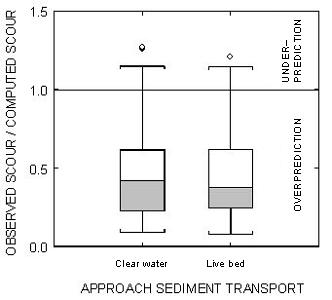
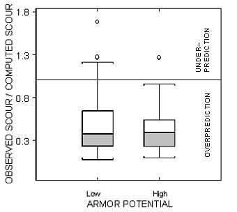
Mueller's K₄, as adopted by the fourth edition of HEC-18, is compared with the expanded data set presented in this report in figure 24.⁽⁵⁾ The equation envelops the data, with the exception of five points. Four of the points underpredicted the observed scour by less than 5 percent. Of the five points lying above the envelope curve in figure 24, four observations are from streams in Ohio. The bridge scour data sets from Ohio contained extensive bed material data, which were collected annually during low flow at most sites. These data included composite samples collected at the bridge and in the approach cross sections and local samples collected at each pier (inside the scour hole, if one were present). The bed material size reported with the scour measurement was usually the sample collected at the pier for the low flow preceding the scour measurement. All four observations for Ohio plotted below the envelope curve if the composite samples were used.

Molinas derived a new correction to the HEC-18 equation from his final laboratory data set.⁽¹⁾ Although several of the terms are similar to those used by Mueller and Jones,⁽⁷⁸⁾ Molinas redefined the equations for computing the incipient motion velocity and the approach velocity causing incipient motion at the pier (see table 3). Although this new correction provided a significant decrease in the sum of squared errors (from 822 to 495), it also significantly increased the number of observations that were underpredicted (from 13 to 65). Figure 13 showed that most of these underpredictions occurred at D₅₀ less than 2 mm. If the correction developed by Molinas is only applied to D₅₀ greater than 2 mm, its performance was enhanced greatly. The sum of squared errors rose to 609, but the number of observations underpredicted dropped from 65 to 21, and the sum of squared errors for the underpredictions was reduced from 17 to 2.47.

Development of New Methodology

Patterns in the performance of the HEC-18 equation clearly show the need for a K₄ term to correct the depth of scour, particularly for coarse bed materials. The HEC-18 equation showed no difference in its performance for clear water or live bed conditions (figure 25). Armoring of the scour hole could cause overpredictions by the HEC-18 equation for coarse bed material. The ability of the flow to transport the D₉₅ sediment size at the pier (estimated using equation 2) was used to determine whether an armor layer would form in the scour hole and limit the depth of scour. Figure 26 shows that there is little difference in the idealized K₄ term (observed depth of scour/HEC-18 computed depth of scour) for conditions where the armoring potential is high. Mueller observed the HEC-18 equation consistently overpredicted scour in coarse bed materials.⁽⁵⁾ Figure 27 clearly shows that for this data set, the magnitude of the overprediction increases with the median bed material size. A wide variation in the depth of scour for sand is indicated by the long whiskers in the box plot.

The K₄ term was developed by evaluating both the whole data set and only the portion with median grain sizes coarser than sand. Figure 28 shows that the depth of scour computed from the HEC-18 equation overpredicts by a larger ratio as the bed material size increases. It is interesting that there is also a negative trend in the approach velocity; this trend would indicate that the HEC-18 equation may have too high an exponent on velocity. The K₄ term should be dimensionless to maintain the dimensional homogeneity of the HEC-18 equation. Numerous combinations of variables were investigated, and the best correlation was found with the median size of the sediment relative to the pier width (b/D₅₀). The equation for the envelope curve using this variable combination is:

(40)

Figure 25 .Box plot of the variation in the ratio of the observed depth of pier scour to the depth of pier scour computed by the HEC-18 equation (idealized K4) for clear water and live bed conditions.

Figure 26. Box plot of the variation in the ratio of the observed depth of pier scour to the depth of pier scour computed by the HEC-18 equation (idealized K4) for low and high armor potential conditions.

Figure 27. Box plot of the variation in the ratio of the observed depth of pier scour to the depth of pier scour computed by the HEC-18 equation (idealized K4) for sediment size classes.

Figure 28. Relation between the ratio of the observed depth of pier scour to the depth of pier scour computed by the HEC-18 equation (idealized K4) and selected variables.

Figure 29 shows the envelope curve for K₄ developed from the b/D₅₀ ratio. This curve is applicable for all grain sizes and appears to explain some of the underprediction for the HEC-18 equation for the sand sizes. If this correction is applied to all observations, the 13 observations that HEC-18 originally underpredicted (table 5) are corrected, but the sum of squared errors increases to over 2,800. The large increase in the sum of squared errors is caused by the large scatter below the curve for values of K₄ above 1. If the correction is limited to reducing the depth of scour (K₄<1), the sum of squared errors is reduced to 611, but 14 observations are underpredicted. The sum of squared errors for the 14 observations underpredicted is 2.16, the same as the HEC-18 equation before this correction (table 5). Use of only bed material size to develop a dimensionally dependent equation reduced the sum of squared errors to 520; this reduction does not seem sufficient to justify the use of a dimensionally dependent equation to compute a K₄ term.

Although the K₄ based on b/D₅₀does not perform as well as the HEC-18-K4Mu equation in table 5, the basis for this new approach is supported to an extent by the work of Sheppard, who found that b/D₅₀ was an important parameter based on his laboratory research.⁽⁶⁴⁾

Figure 29. Relation between relative errors in computed scour using the HEC-18 equation and relative bed material size.

Importance of Sampling Bed Material

The four observations from Ohio above the envelope curve in figure 24 could be reduced or eliminated by use of the grain sizes associated with a composite sample or an average of all available composite samples. While this analysis highlights the sensitivity of Mueller's 1996 K₄ to the bed material samples, it also illustrates the importance of and uncertainty associated with determining bed material characteristics for field conditions.

The potential variability associated with characterizing the bed material can be illustrated using the Ohio bridge scour data sets. These data sets contain 419 samples of bed material, of which 149 represent composite samples for an entire cross section and the rest are point samples near the piers. Table 8 shows that individual samples can vary greatly; the average coefficient of variation is just over 1.0 for all samples, including the composite samples. If only the composite samples are considered, the variability is reduced, but the average coefficient of variation exceeds 0.7. This magnitude of variability is probably responsible for much of the scatter in the relation between depth of scour and bed material characteristics. Even if the perfect scour equation were developed, the variability of bed material characteristics used for input could result in a wide range of scour predictions, depending on the sensitivity of the equation to the bed material characteristics. Therefore, as scour equations are improved by accounting for the effect of bed material characteristics, there will be a commensurate need to ensure that sampling procedures provide representative characteristics of the bed material. If representative bed material characteristics are not obtained, the potential improvements in scour prediction will not be realized.

Back to Top

Previous | Table of Contents | Next