This report is an archived publication and may contain dated technical, contact, and link information

Federal Highway Administration >
Publications >
Research Publications >
03060 >
Appa.Cfm
Concrete Mixture Optimization Using Statistical Methods

Publication Number: FHWA-RD-03-060

Concrete Mixture Optimization Using Statistical Methods

APPENDIX A. Experiment Design and Data Analysis for Mixture Experiment

A.1 Experiment Design and Response Data

Table A-1. Mixture experiment design in terms of volume fractions of components

Standard Order	Design ID	Run Order	A Water	B Cement	C Silica Fume	D HRWRA	E Coarse Agg	F Fine Agg
35	127	1	0.1720	0.1395	0.0130	0.0060	0.4098	0.2598
7	15	2	0.1656	0.1500	0.0270	0.0074	0.4000	0.2500
14	38	3	0.1767	0.1417	0.0270	0.0046	0.4000	0.2500
11	22	4	0.1850	0.1474	0.0130	0.0046	0.4000	0.2500
22	71	5	0.1600	0.1500	0.0130	0.0074	0.4098	0.2598
4	11	6	0.1850	0.1300	0.0130	0.0046	0.4174	0.2500
2	5	7	0.1600	0.1300	0.0270	0.0046	0.4284	0.2500
8	16	8	0.1600	0.1300	0.0130	0.0046	0.4424	0.2500
27	91	9	0.1850	0.1300	0.0130	0.0074	0.4073	0.2573
29	101	10	0.1712	0.1500	0.0130	0.0046	0.4112	0.2500
24	78	11	0.1850	0.1300	0.0270	0.0074	0.4003	0.2503
37	127	12	0.1720	0.1395	0.0130	0.0060	0.4098	0.2598
9	20	13	0.1850	0.1300	0.0130	0.0046	0.4000	0.2674
30	103	14	0.1600	0.1500	0.0130	0.0060	0.4210	0.2500
5	13	15	0.1600	0.1300	0.0130	0.0046	0.4000	0.2924
12	28	16	0.1600	0.1300	0.0270	0.0046	0.4000	0.2784
28	98	17	0.1600	0.1400	0.0130	0.0046	0.4324	0.2500
36	127	18	0.1720	0.1395	0.0130	0.0060	0.4098	0.2598
26	89	19	0.1600	0.1400	0.0130	0.0046	0.4000	0.2824
39	163	20	0.1656	0.1343	0.0165	0.0067	0.4234	0.2536
31	110	21	0.1712	0.1500	0.0130	0.0046	0.4000	0.2612
1	5	22	0.1600	0.1300	0.0270	0.0046	0.4284	0.2500
3	11	23	0.1850	0.1300	0.0130	0.0046	0.4174	0.2500
25	87	24	0.1600	0.1300	0.0130	0.0046	0.4212	0.2712
20	66	25	0.1600	0.1300	0.0270	0.0074	0.4128	0.2628
16	38	26	0.1767	0.1417	0.0270	0.0046	0.4000	0.2500
18	63	27	0.1725	0.1300	0.0270	0.0074	0.4131	0.2500
17	48	28	0.1725	0.1300	0.0130	0.0074	0.4000	0.2771
21	70	29	0.1600	0.1500	0.0130	0.0060	0.4000	0.2710
13	37	30	0.1600	0.1400	0.0270	0.0074	0.4000	0.2656
19	65	31	0.1600	0.1400	0.0270	0.0074	0.4156	0.2500
38	127	32	0.1720	0.1395	0.0130	0.0060	0.4098	0.2598
32	116	33	0.1725	0.1300	0.0270	0.0074	0.4000	0.2631
10	20	34	0.1850	0.1300	0.0130	0.0046	0.4000	0.2674
23	71	35	0.1600	0.1500	0.0130	0.0074	0.4098	0.2598
33	123	36	0.1600	0.1400	0.0200	0.0060	0.4120	0.2620
34	127	37	0.1720	0.1395	0.0130	0.0060	0.4098	0.2598
6	15	38	0.1656	0.1500	0.0270	0.0074	0.4000	0.2500
15	38	39	0.1767	0.1417	0.0270	0.0046	0.4000	0.2500

Table A-2. Mixture experiment: slump and 1-day strength data

Obs	Design ID	Run Order	Slump (mm)		1-Day Strength (MPa)
32	127	1	50.8	54.0	24.3	24.4	24.0	-
6	15	2	25.4	31.8	24.6	22.9	25.9	-
13	38	3	19.1	19.1	22.7	22.6	22.1	-
10	22	4	69.9	63.5	21.1	21.4	21.8	-
20	71	5	63.5	50.8	26.9	27.2	26.5	27.5
3	11	6	108.0	95.3	16.7	16.6	17.0	-
1	5	7	12.7	12.7	21.7	23.3	22.2	-
7	16	8	38.1	31.8	21.8	21.6	21.4	-
25	91	9	203.2	196.9	17.1	16.6	16.7	-
27	101	10	25.4	19.1	26.4	26.5	26.8	-
22	78	11	127.0	127.0	19.2	19.3	19.0	-
33	127	12	101.6	95.3	20.8	21.9	21.9	-
8	20	13	114.3	120.7	18.3	18.0	18.3	-
28	103	14	63.5	63.5	28.0	26.8	27.3	-
5	13	15	63.5	50.8	22.7	21.7	21.0	-
11	28	16	31.8	25.4	21.1	22.9	22.5	-
26	98	17	31.8	31.8	25.2	26.4	24.2	-
34	127	18	95.3	88.9	21.5	21.6	23.8	-
24	89	19	38.1	38.1	18.1	23.1	24.0	-
36	163	20	95.3	95.3	22.1	21.6	22.4	-
29	110	21	50.8	50.8	24.5	25.1	24.4	-
2	5	22	25.4	25.4	22.1	24.0	24.2	-
4	11	23	114.3	114.3	17.1	16.5	15.9	-
23	87	24	63.5	69.9	24.9	20.6	23.2	-
18	66	25	76.2	76.2	25.0	24.1	25.1	-
14	38	26	31.8	25.4	22.9	23.6	22.5	-
16	63	27	101.6	95.3	21.6	22.0	21.4	-
15	48	28	177.8	165.1	22.7	22.7	23.7	-
19	70	29	50.8	50.8	27.5	27.3	27.6	-
12	37	30	38.1	31.8	26.8	27.8	27.4	-
17	65	31	31.8	31.8	28.6	25.5	27.6	-
35	127	32	120.7	120.7	22.9	22.2	22.1	-
30	116	33	114.3	114.3	23.9	23.7	24.1	-
9	20	34	127.0	127.0	18.8	18.6	18.5	-
21	71	35	114.3	101.6	29.5	28.0	28.9	-
31	123	36	76.2	69.9	26.2	26.4	27.3	-
32	127	37	101.6	101.6	23.9	24.3	24.2	-
6	15	38	50.8	50.8	29.2	27.6	29.5	-
13	38	39	25.4	25.4	23.3	25.4	22.2	-

Table A-3. Mixture experiment: 28-day strength and RCT charge passed data

Obs	Design ID	Run Order	28-Day Strength (psi)				RCT Charge Passed (coulombs)
32	127	1	51.0	52.5	54.9	-	-	-	-
6	15	2	59.4	58.7	59.5	-	-	-	-
13	38	3	50.8	50.1	52.7	-	-	-	-
10	22	4	47.9	48.0	48.8	-	1203	1310	1321
20	71	5	51.9	56.7	57.0	-	901	790	894
3	11	6	47.3	51.7	46.6	-	1141	1308	1038
1	5	7	46.1	49.4	49.9	-	422	352	-
7	16	8	54.6	53.2	51.5	-	708	-	843
25	91	9	58.8	60.4	62.1	-	1092	1113	877
27	101	10	57.0	52.3	51.6	-	730	736	767
22	78	11	51.0	55.4	48.6	-	474	454	549
33	127	12	51.1	52.3	47.4	-	853	885	789
8	20	13	51.9	50.2	50.7	-	995	922	793
28	103	14	60.4	56.6	46.2	55.1	607	576	565
5	13	15	51.0	55.6	52.8	-	575	719	758
11	28	16	56.5	50.8	53.4	-	327	268	282
26	98	17	55.5	50.5	49.8	-	580	579	653
34	127	18	53.7	54.2	54.3	-	841	852	848
24	89	19	52.6	58.3	50.2	56.3	677	656	826
36	163	20	61.1	61.0	60.2	-	544	552	566
29	110	21	52.3	52.9	54.4	-	716	804	857
2	5	22	56.3	52.0	53.9	-	308	441	296
4	11	23	49.2	47.8	46.9	-	894	1054	956
23	87	24	53.0	50.4	49.4	-	751	618	732
18	66	25	57.1	62.6	59.7	-	326	319	303
14	38	26	57.4	51.8	50.3	-	450	346	375
16	63	27	56.6	54.5	54.5	-	324	324	257
15	48	28	58.9	58.0	57.3	-	622	702	723
19	70	29	54.7	52.5	56.4	-	496	494	524
12	37	30	49.2	57.8	59.7	57.4	247	254	234
17	65	31	53.5	49.1	50.8	-	285	350	296
35	127	32	57.8	58.6	55.0	-	661	567	680
30	116	33	57.8	57.3	53.5	-	367	358	343
9	20	34	51.1	51.9	51.9	-	804	901	754
21	71	35	64.9	65.6	65.2	-	550	566	543
31	123	36	61.5	59.8	61.8	-	318	312	390
32	127	37	53.8	55.4	54.6	-	640	614	665
6	15	38	61.6	57.5	55.2	-	235	232	250
13	38	39	54.5	53.8	55.4	-	323	379	293

A.2 Data Analysis and Model Fitting

A.2.1 Slump

Table A-4. Mixture experiment: sequential model sum of squares for slump

Source	Sum of Squares	DF	Mean Square	F Value	Prob > F
Mean	212697.8	1	212697.8	-	-
Linear	62543.72	5	12508.74	45.64	< 0.0001
Quadratic	4107.07	15	273.80	1.00	0.5016
Special cubic (aliased)	2164.86	7	309.27	1.27	0.3703
Cubic (aliased)	0.00	0		-	-
Residual	1950.91	8	243.86	-	-
Total	283464.3	36	7874.01	-	-

Table A-5. Mixture experiment: lack-of-fit test for slump

Source	Sum of Squares	DF	Mean Square	F Value	Prob > F
Linear	6271.93	22	285.09	1.17	0.4335
Quadratic	2164.86	7	309.27	1.27	0.3703
Special cubic (aliased)	0.00	0	-	-	-
Cubic (aliased)	0.00	0	-	-	-
Pure error	1950.91	8	243.86	-	-

Table A-6. Mixture experiment: model summary statistics for slump

Source	Std. Dev.	r²	Adj. r²	Pred. r²	PRESS
Linear	16.56	0.8838	0.8644	0.8407	11272.43
Quadratic	16.56	0.9418	0.8643	0.6049	27956.70
Special cubic (aliased)	15.62	0.9724	0.8794	-	undefined
Cubic (aliased)	-	-	-	-	undefined

Table A-7. Mixture experiment: ANOVA for slump mixture model

Source	Sum of Squares	DF	Mean Square	F Value	Prob > F
Model	62543.72	5	12508.74	45.64	< 0.0001
Linear mixture	62543.72	5	12508.74	45.64	< 0.0001
Residual	8222.84	30	274.09	-	-
Lack of fit	6271.93	22	285.09	1.17	0.4335
Pure error	1950.91	8	243.86	-	-
Corrected total	70766.56	35	-	-	-

Table A-8. Mixture experiment: coefficient estimates for slump mixture model

Component	Coeff. Estimate	DF	Std. Error	95% CI Low	95% CI High
Water	155.68	1	10.12	135.03	176.34
Cement	-37.53	1	13.34	-64.77	-10.30
Silica fume	-80.39	1	17.95	-117.04	-43.74
HRWRA	1092.78	1	100.02	888.51	1297.04
Coarse aaggregate	55.14	1	8.85	37.07	73.22
Fine aaggregate	71.03	1	9.29	52.06	90.00

Table A-9. Mixture experiment: adjusted effects for slump mixture model

Component	Adjusted Effect	DF	Std. Error	Approx. t for H_o Effect = 0	Prob > t
Water	-138.04	1	12.96	-2.94	0.0063
Cement	-139.80	1	12.43	-11.25	< 0.0001
Silica fume	-114.84	1	10.42	-11.02	< 0.0001
HRWRA	70.00	1	6.83	10.25	< 0.0001
Coarse aaggregate	-185.17	1	20.68	-8.95	< 0.0001
Fine aaggregate	-166.11	1	22.02	-7.54	< 0.0001

Model equation in terms of pseudocomponents:

Slump = 155.68*A - 37.53*B - 80.39*C + 1092.78*D + 55.14*E + 71.03*F

Model equation in terms of real components:

Slump = 2166.5*water - 2390.5*cement - 3401.2*silica fume + 24267.7*HRWRA - 204.8*Coarse agg +169.9*Fine agg

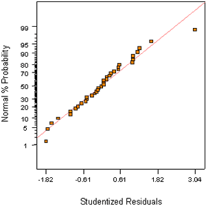
Figure A-1. Mixture experiment: normal probability plot for slump

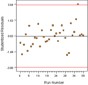
Figure A-2. Mixture experiment: residuals versus run for slump. Chart. In this figure, the residuals are plotted on the Y-axis against the corresponding runs on the X-axis. In this plot, the residuals show a slight upward trend with time, but probably not significant.

Figure A-2. Mixture experiment: residuals vs. run for slump

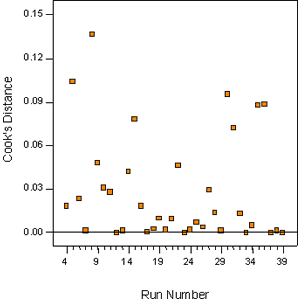
Figure A-3. Mixture experiment: Cook's distance for slump

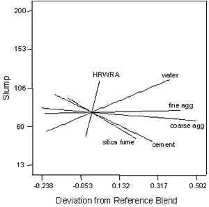
Figure A-4. Mixture experiment: trace plot for slump

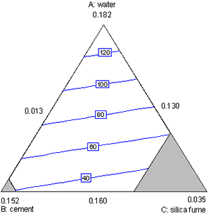
Figure A-5. Mixture experiment: contour plot for slump in water, cement, and silica fume

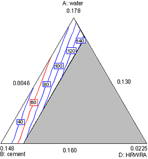
Figure A-6. Mixture experiment: contour plot of slump in water, cement, and HRWRA

A.2.2 1-Day Strength

Table A-10. Mixture experiment: sequential model sum of squares for 1-day strength

Source	Sum of Squares	DF	Mean Square	F Value	Prob > F
Mean	19278.40	1	19278.40	-	-
Linear	351.33	5	70.27	57.34	< 0.0001
Quadratic	27.14	15	1.81	2.82	0.0266
Special cubic (aliased)	3.43	7	0.49	0.63	0.7199
Cubic (aliased)	0.00	0	-	-	-
Residual	6.19	8	0.77	-	-
Total	19666.48	36	546.29	-	-

Table A-11. Mixture experiment: lack-of-fit test for 1-day strength

Source	Sum of Squares	DF	Mean Square	F Value	Prob > F
Linear	30.57	22	1.39	1.79	0.1992
Quadratic	3.43	7	0.49	0.63	0.7199
Special cubic (aliased)	0.000	0	-	-	-
Cubic (aliased)	0.000	0	-	-	-
Pure error	6.19	8	0.77	-	-

Table A-12. Mixture experiment: summary statistics for 1-day strength

Source	Std. Dev.	r²	Adj. r²	Pred. r²	PRESS
Linear	1.11	0.9053	0.8895	0.8611	53.89
Quadratic	0.80	0.9752	0.9421	0.8566	55.65
Special cubic (aliased)	0.88	0.9840	0.9302	-	undefined
Cubic (aliased)	-	-	-	-	undefined

Table A-13. Mixture experiment: ANOVA for 1-day strength mixture model

Source	Sum of Squares	DF	Mean Square	F Value	Prob > F
Model	373.09	9	41.45	71.84	< 0.0001
Linear mixture	351.77	5	70.35	121.93	< 0.0001
AF	4.14	1	4.14	7.18	0.0126
BF	5.38	1	5.38	9.32	0.0052
CD	3.96	1	3.96	6.86	0.0145
DF	7.83	1	7.83	13.58	0.0011
Residual	15.00	26	0.58	-	-
Lack of fit	8.81	18	0.49	0.63	0.8010
Pure error	6.19	8	0.77	-	-
Corrected total	388.09	35	-	-	-

Table A-14. Mixture experiment: coefficient estimates for 1-day strength mixture model

Component	Coeff. Estimate	DF	Std. Error	95% CI Low	95% CI High
water	12.93	1	0.62	11.64	14.21
Cement	35.42	1	0.83	33.72	37.12
Silica fume	24.89	1	1.15	22.52	27.25
HRWRA	10.83	1	8.88	-7.42	29.07
Coarse aaggregate	22.04	1	0.43	21.16	22.93
Fine aaggregate	21.50	1	0.57	20.32	22.67
Water-fine aaggregate	7.58	1	2.83	1.77	13.39
Cement-fine aaggregate	-10.07	1	3.30	-16.86	-3.29
Silica fume-HRWRA	78.71	1	30.04	16.95	140.47
HRWRA-fine aaggregate	80.50	1	21.85	35.60	125.41

Model equation in terms of pseudocomponents:

Slump = 12.93*A + 35.42*B + 24.89*C + 10.83*D + 22.04*E + 21.50*F + 7.58* A*F - 10.07*B*F + 78.71*C*D + 80.50*D*F

Model equation in terms of real components:

Slump =	-1209.1water + 1775.9cement - 74.71SF - 11969HRWRA
	+ 59.59Coarse agg - 105.24Fine agg + 4214.9waterFine agg
	- 5603.1cementFine agg + 43782 SFHRWRA + 44781HRWRAFine agg

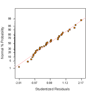
Figure A-7. Mixture experiment: normal probability plot for 1-day strength

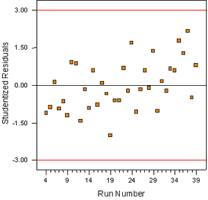
Figure A-8. Mixture experiment: residuals versus run for 1-day strength. Chart. This figure shows a plot of residuals versus run for 1-day strength. The residuals are plotted on the Y-axis against the corresponding runs on the X-axis. The residuals show a slight but insignificant curvelinear trend

Figure A-8. Mixture experiment: residuals vs. run for 1-day strength

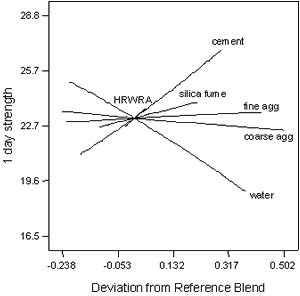
Figure A-9. Mixture experiment: trace plot for 1-day strength

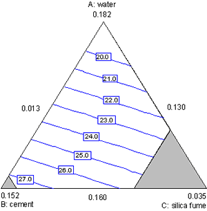
Figure A-10. Mixture experiment: contour plot of 1-day strength in water, cement, and silica fume

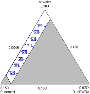
Figure A-11. Mixture experiment: contour plot of 1-day strength in water, cement, and HRWRA

Figure A-12. Mixture experiment: contour plot of 1-day strength in water, cement, and fine aaggregate

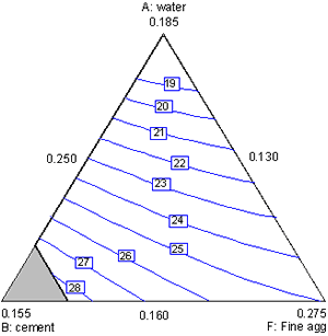
Figure A-13. Mixture experiment: contour plot of 1-day strength in silica fume, HRWRA, and fine aaggregate

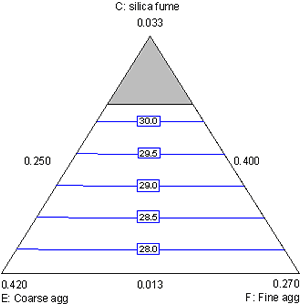
Figure A-14. Mixture experiment: contour plot of 1-day strength in silica fume, coarse aaggregate, and fine aaggregate

A.2.3 28-Day Strength

Table A-15. Mixture experiment: sequential model sum of squares for 28-day strength

Source	Sum of Squares	DF	Mean Square	F Value	Prob > F
Mean	106213.0	1	106213.0	-	-
Linear	257.52	5	51.50	5.46	0.0011
Quadratic	135.19	15	9.01	0.92	0.5665
Special cubic (aliased)	55.45	7	7.92	0.69	0.6826
Cubic (aliased)	0.00	0	-	-	-
Residual	92.17	8	11.52	-	-
Total	106753.3	36	2965.37	-	-

Table A-16. Mixture experiment: lack-of-fit test for 28-day strength

Source	Sum of Squares	DF	Mean Square	F Value	Prob > F
Linear	190.64	22	8.67	0.75	0.7193
Quadratic	55.45	7	7.92	0.69	0.6826
Special cubic (aliased)	0.00	0	-	-	-
Cubic (aliased)	0.00	0	-	-	-
Pure error	92.17	8	11.52	-	-

Table A-17. Mixture experiment: model summary statistics for 28-day strength

Source	Std. Dev.	r²	Adj. r²	Pred. r²	PRESS
Linear	3.07	0.4755	0.3894	0.2678	395.63
Quadratic	3.14	0.7268	0.3625	-1.5516	1378.72
Special cubic (aliased)	3.39	0.8294	0.2537	-	undefined
Cubic (aliased)	-	-	-	-	undefined

Table A-18. Mixture experiment: ANOVA for 28-day strength mixture model

Source	Sum of Squares	DF	Mean Square	F Value	Prob > F
Model	257.52	5	51.50	5.46	0.0011
Linear mixture	257.52	5	51.50	5.46	0.0011
Residual	282.81	30	9.43	-	-
Lack of fit	190.64	22	8.67	0.75	0.7193
Pure error	92.17	8	11.52	-	-
Corrected total	540.33	35	-	-	-

Table A-19. Mixture experiment: estimated coefficients for 28-day strength mixture model

Component	Coeff. Estimate	DF	Std. Error	95% CI Low	95% CI High
Water	48.60	1	1.88	44.77	52.43
Cement	54.30	1	2.47	49.25	59.35
Silica fume	50.36	1	3.33	43.56	57.15
HRWRA	134.13	1	18.55	96.24	172.01
Coarse aaggregate	52.14	1	1.64	48.79	55.50
Fine aaggregate	54.21	1	1.72	50.70	57.73

Table A-20. Mixture experiment: adjusted effects for 28-day strength mixture model

Component	Adjusted Effect	DF	Std. Error	Approx. t for H_o Effect = 0	Prob > t
Water	-12.04	1	2.40	-5.01	< 0.0001
Cement	-6.41	1	2.31	-2.78	0.0093
Silica fume	-6.05	1	1.93	-3.13	0.0039
HRWRA	5.43	1	1.27	4.28	0.0002
Coarse aaggregate	-16.17	1	3.84	-4.22	0.0002
Fine aaggregate	-13.69	1	4.08	-3.35	0.0022

Model equation in terms of pseudocomponents:

28-Day Strength = 48.60*A + 54.30*B + 50.36*C + 134.13*D + 52.14*E + 54.21*F

Model equation in terms of real components:

28-Day Strength = -45.22*water + 89.15*cement - 3.809*silica fume + 1972*HRWRA + 38.36*Coarse agg + 87.19*Fine agg

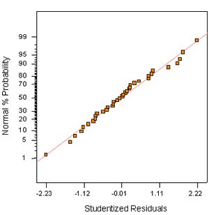
Figure A-15. Mixture experiment: normal probability plot for 28-day strength

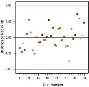
Figure A-16. Mixture experiment: residuals versus run for 28-day strength. Chart. This figure shows a plot of residuals versus run for 28-day strength. The residuals are plotted on the Y-axis against the corresponding runs on the X-axis. The residuals show no structure (they are randomly distributed about a horizontal line).

Figure A-16. Mixture experiment: residuals vs. run for 28-day strength

Figure A-17. Mixture experiment: Cook's distance versus run for 28-day strength. Chart. This figure shows Cook's distance (Y-axis) versus run (X-axis) for 28-day strength. Cook's distance assesses the influence that outlier data points have on the fitted regression function. According to this plot, the maximum value of Cook's distance for this model is 0.17, which indicates that the outlier points do not have significant effects on the regression model.

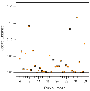
Figure A-17. Mixture experiment: Cook's distance vs. run for 28-day strength

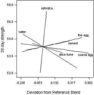
Figure A-18. Mixture experiment: trace plot for 28-day strength

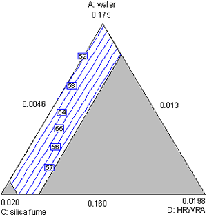
Figure A-19. Mixture experiment: contour plot of 28-day strength in water, silica fume, and HRWRA

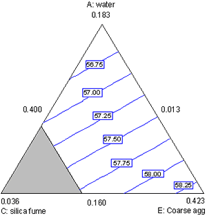
Figure A-20. Mixture experiment: contour plot of 28-day strength in water, silica fume, and coarse aaggregate

Figure A-21. Mixture experiment: contour plot of 28-day strength in cement, coarse aaggregate, and fine aaggregate. Diagram. This figure shows a contour plot of 28-day strength in cement, coarse aaggregate, and fine aaggregate. Cement is the top vertex of the triangular plot, with coarse aaggregate at the lower left, and fine aaggregate at the lower right. The vertices represent the high settings of each component. The strength contours increase from bottom left to upper right with increasing cement, decreasing coarse aaggregate, and increasing fine aaggregate.

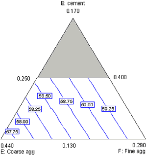
Figure A-21. Mixture experiment: contour plot of 28-day strength in cement, coarse aaggregate, and fine aggregate

A.2.4 RCT Charge Passed

Table A-21. Mixture experiment: sequential model sum of squares for RCT charge passed

Source	Sum of Squares	DF	Mean Square	F Value	Prob > F
Mean	1441.26	1	1441.26	-	-
Linear	6.75	5	1.35	57.33	< 0.0001
Quadratic	0.38	15	0.03	1.17	0.3846
Special cubic (aliased)	0.11	7	0.02	0.57	0.7607
Cubic (aliased)	0.00	0	-	-	-
Residual	0.22	8	0.03	-	-
Total	1448.72	36	40.24	-	-

Table A-22. Mixture experiment: lack-of-fit test for RCT charge passed

Source	Sum of Squares	DF	Mean Square	F Value	Prob > F
Linear	0.490	22	0.022	0.82	0.6666
Quadratic	0.109	7	0.016	0.57	0.7607
Special cubic (aliased)	0.000	0	-	-	-
Cubic (aliased)	0.000	0	-	-	-
Pure error	0.217	8	0.027	-	-

Table A-23. Mixture experiment: model summary statistics for RCT charge passed

Source	Std. Dev.	r²	Adj. r²	Pred. r²	PRESS
Linear	0.15	0.9053	0.8895	0.8647	1.01
Quadratic	0.15	0.9563	0.8980	0.8044	1.46
Special cubic (aliased)	0.16	0.9709	0.8726	-	undefined
Cubic (aliased)	-	-	-	-	undefined

Table A-24. Mixture experiment: ANOVA for RCT charge passed mixture model

Source	Sum of Squares	DF	Mean Square	F Value	Prob > F
Model	6.75	5	1.35	57.33	< 0.0001
Linear mixture	6.75	5	1.35	57.33	< 0.0001
Residual	0.71	30	0.024	-	-
Lack of fit	0.49	22	0.022	0.82	0.6666
Pure error	0.22	8	0.027	-	-
Corrected total	7.46	35	-	-	-

Table A-25. Mixture experiment: estimated coefficients for RCT charge passed mixture model

Component	Coeff. Estimate	DF	Std. Error	95% CI Low	95% CI High
Water	7.2	1	0.094	7.01	7.39
Cement	6.34	1	0.12	6.09	6.60
Silica fume	4.10	1	0.17	3.76	4.44
HRWRA	5.32	1	0.93	3.43	7.22
Coarse aaggregate	6.62	1	0.082	6.46	6.79
Fine aaggregate	6.45	1	0.086	6.28	6.63

Table A-26. Mixture experiment: adjusted effects for RCT charge passed mixture model

Component	Adjusted Effect	DF	Std. Error	Approx. t for H_o Effect = 0	Prob > t
Water	0.84	1	0.12	7.03	< 0.0001
Cement	0.19	1	0.12	1.65	0.1087
Silica fume	-0.76	1	0.097	-7.83	< 0.0001
HRWRA	-0.054	1	0.063	-0.85	0.3999
Coarse aaggregate	0.74	1	0.19	3.86	0.0006
Fine aaggregate	0.53	1	0.20	2.62	0.0138

Model equation in terms of pseudocomponents:

ln(RCT charge passed) = 7.20*A + 6.34*B + 4.10*C + 5.32*D + 6.62*E + 6.45*F

Model equation in terms of real components:

ln(RCT charge passed) = 20.82*water + 0.629*cement - 52.33*silica fume - 23.41*HRWRA + 7.235*Coarse agg + 3.190*Fine agg

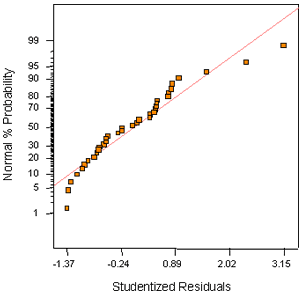
Figure A-22. Mixture experiment: normal probability plot for RCT charge passed (no transform)

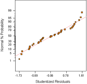
Figure A-23. Mixture experiment: normal probability plot for RCT charge passed (natural log transform)

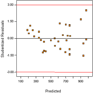
Figure A-24. Mixture experiment: residuals versus predicted for RCT charge passed (no transform). Chart. This figure shows a plot of residuals versus predicted values for RCT (with no transform). The residuals are plotted on the Y-axis against the corresponding predicted values on the X-axis. The desired appearance of this plot is a uniform range in the residuals over the range of predicted values. With no transform, the range of residuals increases with increasing predicted value.

Figure A-24. Mixture experiment: residuals vs. predicted for RCT charge passed (no transform)

Figure A-25. Mixture experiment: residuals versus run for RCT charge passed (no transform). Chart. This figure shows residuals versus run for RCT (no transform). The residuals are plotted on the Y-axis against the corresponding runs on the X-axis. For these data, there appears to be a curvelinear structure to the residuals.

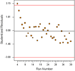
Figure A-25. Mixture experiment: residuals vs. run for RCT charge passed (no transform)

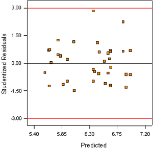
Figure A-26. Mixture experiment: residuals vs. predicted for RCT charge passed (natural log transform)

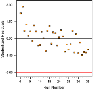
Figure A-27. Mixture experiment: residuals vs. run for RCT charge passed (natural log transform)

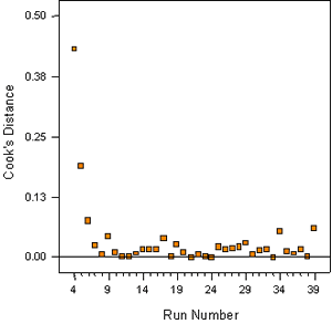
Figure A-28. Mixture experiment: Cook's distance for RCT charge passed (natural log transform)

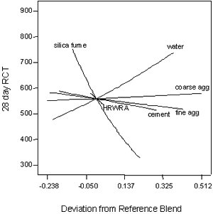
Figure A-29. Mixture experiment: trace plot for RCT charge passed (natural log transform)

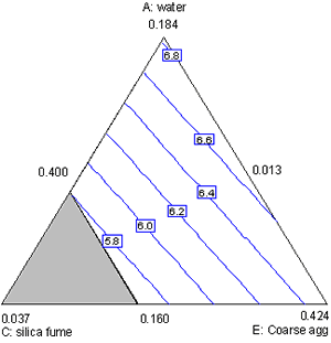
Figure A-30. Mixture experiment: contour plot of ln (RCT charge passed) in water, silica fume, and coarse aaggregate

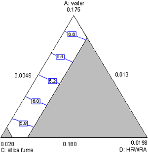
Figure A-31. Mixture experiment: contour plot of ln (RCT charge passed) in water, silica fume, and HRWRA

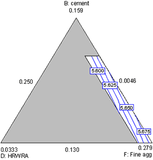
Figure A-32. Mixture experiment: contour plot of ln (RCT charge passed) in cement, HRWRA, and fine aaggregate

Previous | Table of Contents | Next

Page Owner: Office of Research, Development, and Technology, Office of Infrastructure, RDT

Topics: research, infrastructure, pavements and materials
Keywords: research, infrastructure, pavements and materials, High Performance Concrete Pavement; HIPERPAV; Jointed; Continuously Reinforced; Early-Age Behavior; Long-Term Performance; Mechanistic-Empirical Models; Temperature; Hydration; Shrinkage; Relaxation; Creep; Thermal Expansion; Slab Base Restraint; Curling; Warping; Plastic Shrinkage; Cracking; JPCP; CRCP
TRT Terms: research, facilities, transportation, highway facilities, roads, parts of roads, pavements
Scheduled Update: Archive - No Update needed

This page last modified on 03/08/2016

Slump =	-1209.1water + 1775.9cement - 74.71SF - 11969HRWRA
	+ 59.59Coarse agg - 105.24Fine agg + 4214.9waterFine agg
	- 5603.1cementFine agg + 43782 SFHRWRA + 44781HRWRAFine agg