Concrete Mixture Optimization Using Statistical Methods

Previous | Table of Contents

APPENDIX C. Cost User's Guide

ABSTRACT

This user's guide provides instructions for and examples of using the Concrete Optimization Software Tool (COST), a joint product of the Federal Highway Administration and the National Institute of Standards and Technology. COST provides an Internet-based system for optimizing concrete performance based on statistical experiment design and analysis methods. Working with local raw materials, COST designs an experimental program of concrete mixtures to be prepared and evaluated. In these mixtures, the user can vary the water-to-cement (w/c) ratio and other concrete mixture parameters such as the cement, mineral and chemical admixture, and aggregate contents. Once the measured responses (properties) for the prepared concretes are input into the COST system, it analyzes the results and determines the optimum mixture proportions based on user-supplied performance criteria. Results and analysis are provided in both graphical and numerical formats to aid in interpretation. Typical uses of COST might be to design a concrete that meets all specifications at minimum cost or to design a concrete that provides maximum durability within a specific cost range.

Keywords: Building technology, concrete, experiment design, mixture proportioning, optimization, response surfaces.

SECTION 1
Overview

C1.1 Introduction

In the simplest case, portland cement concrete is a four-component mixture of water, portland cement, fine aggregate, and coarse aggregate. Additional components, such as chemical admixtures (air entraining agents, superplasticizers) and mineral admixtures (coal fly ash, silica fume, blast furnace slag), may be added to the basic mixture to enhance certain properties of the fresh or hardened concrete. High-performance concrete mixtures, which may be required to meet several performance criteria (e.g., compressive strength, elastic moduli, rapid chloride permeability) simultaneously, typically contain at least six components. Thus, optimizing mixture proportions for high-performance concrete, which contains many constituents and is often subject to several performance constraints, can be a difficult and time-consuming task.

The Concrete Optimization Software Tool (COST) is an online interactive system developed to assist engineers, concrete producers, and researchers in optimizing portland cement concrete mixtures for their particular applications. COST applies response surface methodology (RSM), a collection of statistical experiment design and analysis methods, to the problem of optimizing concrete mixture proportions. RSM is often used in industry for product development, formulation, and improvement, and is applicable to problems such as concrete mixture proportioning where several input variables (factors) influence a performance measure (response).

COST is intended to provide an introduction to concrete practitioners who are unfamiliar with the concepts and process of applying RSM to concrete mixture proportioning. COST allows users to learn how RSM can be applied to the problem of optimizing concrete mixtures.

There are two scenarios for which COST could be applied:

• The first, and probably most common, would be the case where a user wants to proportion a concrete mixture to meet a set of specifications at minimum material cost.
• The second is the case where the user wants to maximize (or minimize) a particular response or responses, irrespective of cost.

COST can be used to optimize cement paste, mortar, or concrete mixtures. In all three cases, varying the mixture component proportions affects both fresh and hardened properties of the paste, mortar or concrete. The properties (responses) depend on the proportions of the components. Table C-1 lists examples of typical components and responses for concrete mixtures (components and responses other than those listed can be used).

In COST, the water-cement (w/c) ratio (or water-cementitious materials (w/cm) ratio) is varied along with up to four additional components. These are referred to as variable factors. Other factors may be included in the mixture at fixed (constant) levels, and are referred to as fixed factors. Up to five concrete properties, or responses, (e.g., slump, strength, air content, cost, etc.) can be designated by the user according to the requirements of the application. These concepts are explained more fully in section 2.

Table C-1. Examples of components and responses

COST is accessible via the Internet. The program consists of a front-end HTML interface that allows the user to enter required information. Underlying code (written in C) processes the input, generates the experiment designs and mixture proportions, calls routines for statistical analysis, and generates output. The statistical analysis routines are part of an interactive statistical software package, DATAPLOT, which was developed at the National Institute of Standards and Technology.

C1.2 Scope

COST is not intended to supplant or compete with commercially available experiment design and analysis software packages. Rather, the purpose of COST is to introduce to the concrete practitioner the concepts of statistical experiment design and analysis using RSM and how they might be applied to concrete mixture proportioning. COST is specifically geared toward the application of these methods to concrete mixture proportioning.

This section provides a general overview of the COST program. Section 2 of this manual provides step-by-step instructions for using COST. Section 3 contains a glossary of terms, additional details on the statistical aspects of the experiment designs and analyses used, and a list of references.

C1.3 System Requirements

To use COST, your system must have the following components and settings:

• Personal computer (Pentium®¹ or equivalent) with video card and monitor set for 800 x 600 resolution (min) and 65536 colors.
• Access to the Internet (World Wide Web) and one of the following browsers: Netscape Navigator 4.0 (or above) or Microsoft® Internet Explorer 4.0 (or above). The COST interface uses both frames and JavaScript.

C1.4 Disclaimer

This software was developed at NIST by employees of the Federal Government in the course of their official duties. Pursuant to Title 17, Section 105 of the U.S. Code, this software is not subject to copyright protection and is in the public domain. COST is an experimental system. NIST and the Federal Highway Administration (FHWA) assume no responsibility whatsoever for its use by other parties, and make no guarantees, expressed or implied, about its quality, reliability, or any other characteristic. We would appreciate acknowledgement if the software is used.

The U.S. Department of Commerce and the U.S. Department of Transportation make no warranty, expressed or implied, to users of COST and associated computer programs, and accepts no responsibility for its use. Users of COST assume sole responsibility under Federal law for determining the appropriateness of its use in any particular application; for any conclusions drawn from the results of its use; and for any actions taken or not taken as a result of analyses performed using these tools.

Users are warned that COST is intended for use only by those competent in the field of concrete technology and is intended to supplement the informed judgment of the qualified user. Lack of accurate predictions by the COST models could lead to erroneous conclusions with regard to materials selection and design. All results should be evaluated by an informed user.

C1.5 General Information

C1.5.1 COST Homepage and Main Menu

The COST homepage may be accessed at http://ciks.cbt.nist.gov/cost. The COST homepage is shown in figure C-1.

The homepage contains a brief overview of the COST program. The blue bar on the left side of the screen is the main menu. Menu selections are described briefly below. Details on each step are provided in section 2, "Using COST."

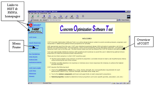
COST Home-allows user to return to the initial screen (figure C-1) at any time.

Specify Responses-user enters information on responses to be measured. Responses are the measured properties of the concrete (fresh or hardened) such as slump, air content, strength, shrinkage, etc., that are specified for the particular project.

Specify Mixtures-user enters information on mixture components and proportions, and COST generates an experimental plan.

View Experimental Plan-user can view a previously generated experimental plan.

Run Trial Batches-contains guidelines for performing the trial batches according to the experimental plan. This step is performed by the user in his/her laboratory, and involves batching, fabricating, curing, and testing specimens. Types of specimens and test methods used will depend on the responses specified in step 1. It is the user's responsibility to determine the appropriate test method to use.

Enter Results-user enters test results for each trial batch and each response.

Analyze Data-COST provides 10 analysis tasks to assist the user in analyzing and interpreting the results. The tasks include checking the experiment design, looking at trends in the data graphically, generating empirical (quadratic) models for each response, and optimizing according to individual runs, means, and models.

Summarize Analysis-summary of main results of analysis.

User's Guide-HTML version of the COST User's Guide. A PDF version is also available for download.

FAQ's-frequently asked questions.

References-a list of references on statistics, response surface methods and DATAPLOT (software used by COST).

Glossary-a glossary of statistical terms.

SECTION 2
Using COST

C2.1 Background and Preliminary Planning

Using COST requires several steps, including planning, running trial batches, entering results, analyzing, interpreting, and summarizing results. These tasks have been divided into the following six steps (as listed in the COST menu):

• Specify responses.
• Specify mixtures.
• Run trial batches.
• Enter results.
• Analyze data.
• Summarize analysis.

In most cases, these steps will be performed in the order listed above. Each step is described in detail in the sections below.

Before starting the six-step process, the user must perform some preliminary steps:

1. Define the overall objective of the project. Typical objectives include the following:
   
   • Minimize cost while meeting several performance criteria for responses.
   • Minimize or maximize a single response or several responses.
     
2. Define the properties (responses) and mixture components (factors) to be included, and define which will be variable or fixed factors. Variable factors include w/c or w/cm plus up to four additional components. Additional factors may be included at fixed levels. See "Background Information" below for further details.
   
3. Define the performance criteria (most likely based on the job specifications) for each response, and the numerical ranges for each factor.
   
4. Collect necessary material information (e.g., properties and costs of each component). The required information for each type of material is listed in table C-2.

C2.1.1 Responses

Responses are the concrete properties of interest that will be measured and compared to specified performance criteria (i.e., limits on allowable values of the responses). The responses are dependent variables; that is, the value of a measured response depends on the settings of the independent variables, or factors (see step 2 below). Responses and performance criteria are often dictated by specifications. For example, the specifications for a particular job may indicate that the concrete must have a slump between 50 mm and 100 mm, an air content between 4.5 percent and 7.5 percent by volume, and 28-day strength greater than 69 MPa. The responses in this case are slump, air content and 28-day strength, and the performance criteria are the ranges of acceptable values of the responses.

C2.1.2 Factors

The factors are the independent variables that affect the measured values of the responses. For concrete mixtures, these factors include mixture proportions (relative amounts of each component material) as well as others related to construction practice and environmental conditions. COST assumes that construction and environmental conditions are fixed (as in the case of a set of laboratory or plant trial batches), so the factors of concern are the mixture proportions for each component.

Concrete can contain a variety of component materials. Allowable material types for this version of COST include the following:

• Water.
• Cement.
• Mineral admixtures (up to 4): fly ash, silica fume, slag, other (user specified).
• Chemical admixtures (up to 3): all user specified.
• Aggregates (up to 3): coarse, fine, other (user specified).

COST always requires that either w/c or w/cm be included as a variable factor. Thus, the two mixture components water and cement are accounted for in this single factor.

Factors may be variable or fixed (set at a constant level). For concrete mixture proportioning, variable factors would usually be the mixture components expected to have the most significant effects on the responses. Fixed factors would be those expected to have little or no effect, and would be held constant in the experiment. Any of the factors included in COST may be set as variable or fixed; however, COST limits the user to a maximum of five variable factors for any one experiment (the greater the number of variable factors, the greater the number of trial batches required). Because w/c or w/cm is always considered to be one factor, up to six material components (water, cement, and four others) may be varied.

For all variable factors, low and high settings, or levels, must be defined. The low and high settings are the range over which the factor will vary. For example, w/c could have a range of 0.35 (low level) to 0.45 (high level), or silica fume could have a range of 5 to 10 percent (cement mass replacement). For fixed factors, a fixed (constant) level is specified.

Table C-2 summarizes the information required for different types of materials.

Once the user has decided on the factors to include, defined their ranges (for variable factors) or constant levels (for fixed factors), and obtained other necessary information (table C-2), the information may be entered into COST to generate a trial batch plan.

In most cases, the selection of components and their ranges is up to the user; however, in some cases, some of the factors and levels may be designated in specifications. For example, a specification may have a maximum w/c, or minimum silica fume content. COST does not provide guidance on the selection of minimum and maximum values for the components.

C2.2 Step 1 - Specify Responses

When "Specify Responses" is selected from the main menu, a form entitled "COST Input Form: Response Information" appears in the right frame. This form is shown in figure C-2.

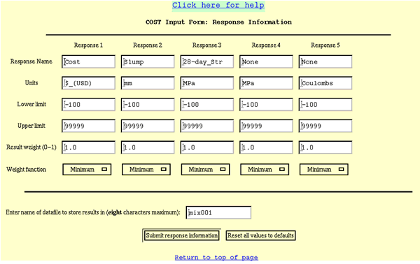
Referring to figure C-2, the following information must be entered into COST for each response:

• A name for the response. The name should be as short as possible (no more than 10 characters) and may include alphanumeric characters and underscores (e.g., slump, 28-day_str). No other characters are allowed.
  
• The units in which the response is measured.
  
• A lower limit for the response, if applicable. This would be a specified minimum value (e.g., minimum 1-day strength of 15 MPa). If there is not a lower limit for the response, a default value of -100 is used.
  
• An upper limit for the response, if applicable. This would be a specified maximum value (e.g., maximum rapid chloride permeability (RCT) test result of 1000 coulombs). If there is no upper limit, a default value of 99999 is used.
  
• A result weight factor between 0 and 1, to indicate the relative importance of the response in optimization, compared to the other responses. A factor of 1 indicates most important. The default value is 1 for all responses. If all responses are of equal importance, use the default values. (Note: to optimize a single response while ignoring all others, set the weight factor of the response of interest to 1 and the weight factors of all others to zero).
  
• The type of weight function to use in optimization. Choices are:
  
  • Minimum value is best (linear decreasing from 1 to 0 over response range).
    
  • Maximum value is best (linear increasing 0 to 1 over response range).
    
  • Target value is best (linear increasing from 0 to 1 over lower half of response range, and decreasing from 1 to 0 over upper half of response range).
    
  • Within range (all values in range are equally acceptable but no values outside range are acceptable).

    The response range is defined by the lower and upper limits specified above, or by the minimum (or maximum) value of the response obtained in the experiment if it is greater than (less than) the lower (upper) limit. A different type of weight function can be specified for each response, if desired.

• A filename for the project, eight characters or fewer (alphanumeric characters only) and no extension. The filename will be unique to a particular project, and COST will create several files using the same filename with different extensions as you proceed through the steps (Note: remember this filename, as it will be needed in subsequent steps as well).

After entering the filename, the user should click on "Submit" to submit the completed form information to COST, or "Reset" to reset all settings to their default values.

C2.3 Step 2-Specify Mixtures

When "Specify Mixtures" is selected from the main menu, a form entitled "COST Input Form: Mixture Factors and Information" appears. Figure C-3 shows the first two sections of this form. The instructions for completing these sections are listed below.

C2.3.1 Instructions for Section 1: Number of Parameters (Factors) to Vary

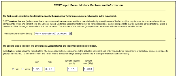
In section 1, the number of parameters (factors) to vary is selected. The user may select 2 to 5 parameters to vary (default is 4). The number of experimental runs is also shown for each selection. The number of experimental runs depends on whether the user includes 3 or 5 center points in the design (the number of center points is entered at the bottom of the form).

• To select the number of parameters to vary, use the pulldown menu.

C2.3.2 Instructions for Section 2: Select w/c or w/cm

In section 2, the user selects w/c or w/cm as a factor, defines the range (low and high settings) for this factor, and enters information about the cement.

• To select w/c or w/cm, click on the radio button next to the desired choice.
  
• Enter the low and high settings of w/c or w/cm (by mass fraction) in the boxes labeled "min" and "max", respectively.
  
• Enter the cement specific gravity.
  
• Enter the cement cost in dollars per kilogram.

C2.3.3 Instructions for Section 3: Select Other Mixture Components

The third section of the form allows selection of other mixture components (mineral admixtures, chemical admixtures, and aggregates). A maximum of four additional variable factors, and any number of fixed factors, may be included. The total number of variable factors selected (including w/c or w/cm, selected in section 2) must match the "number of parameters to vary" selected in section 1.

The additional factors are selected from three types of materials: mineral admixtures, chemical admixtures, and aggregates. Regardless of type, the first task is to indicate whether the factor will be included or not, and if it will be included, whether it will be variable or fixed. This setting is defined using a pulldown menu on the left of the factor name, as described in the following instructions (refer to figure C-4 below):

• To include a component as a variable factor, select "On" in the pulldown menu at the left. Enter the type of material (if not predefined), the low and high settings in the "min" and "max" boxes, and the additional information in the other boxes.
  
• To include a component as a fixed factor (held at a constant level), select "Off" in the pulldown menu on the left, and enter a nonzero fixed setting in the "min" box (the entry in the "max" box will be ignored). Then enter the additional information for each fixed factor in the boxes.
  
• To exclude a component completely, select "Off" in the pulldown menu on the left, and set the value in the "min" box to zero. All other information for these factors is ignored. NOTE: this is the default setting for all factors.

C2.3.4 Specific Instructions for Mineral Admixtures

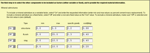
There are three pre-designated mineral admixtures (fly ash, silica fume, and slag), plus one blank for a user-designated choice. Mineral admixtures ranges are defined in terms of percent cement mass replacement. Specific gravity and cost must also be entered.

• Enter the name of the mineral admixture (if the user-defined box is used).
  
• To define the range for a mineral admixture, enter the min and max values in units of percent cement mass replacement.
  
• Enter the specific gravity of the mineral admixture.
  
• Enter the cost of the mineral admixture in dollars per kilogram.
  

C2.3.5 Specific Instructions for Chemical Admixtures

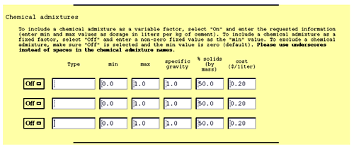
All chemical admixtures are user-designated, and chemical admixtures ranges are defined in terms of dosage rate in liters per kg of cement.

• Enter the name of the chemical admixture.
  
• To define the range for a chemical admixture, enter the min and max values in units of dosage in liters per kilogram of cement (note that this is L/kg, not L/100 kg!!).
  
• Enter the specific gravity of the chemical admixture.
  
• Enter the percent solids (by mass fraction) of the chemical admixture.
  
• Enter the cost of the chemical admixture in dollars per liter.

C2.3.6 Specific Instructions for Aggregates

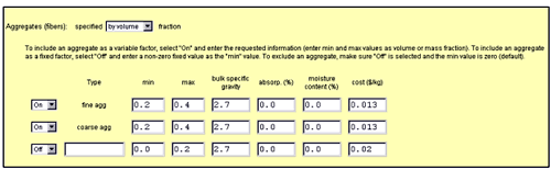
Aggregates include two predesignated types (coarse and fine), and one blank for a user-designated choice. The user-designated choice may be used for an additional aggregate or fibers. Aggregates may be defined in terms of volume fraction or mass fraction. Steps for entering aggregate information (see figure C-6) are as follows:

• Select how the aggregate range will be defined (by volume or by mass) using the pulldown menu at the top of the section (see figure 6).
  
• Enter a name for the aggregate (if the user-defined box is used).
  
• To define the range for the aggregate, enter the min and max values in units of volume fraction or mass fraction (depending on the selection made above).
  
• Enter the bulk specific gravity for the aggregate.
  
• Enter the absorption of the aggregate (in percent by mass of aggregate)
  .
• Enter the moisture content of the aggregate as batched (in percent by mass of aggregate).
  
• Enter the cost of the aggregate in dollars per kilogram.
  

C2.3.7 Instructions for Section 4: Additional Information

In section 4, the user enters additional information needed to generate the trial batch experimental plan. This information includes the number of center points to be run and a random number seed. Steps for entering this information (see figure C-7) are as follows:

• Enter the number of center points to use in the experiment, using the pulldown menu. Center points are experimental runs in which all factors are set at the midpoints of their ranges. The coded values for the low and high settings are -1 and +1, respectively. The coded values for the center points are zero. Center point mixes are replicated to estimate pure error and also may be used as control mixes to assess variation over time. It is a good idea to run at least 3 center points to assess this variation.
  
• Enter a random number seed (any number less than zero). This is used to generate a random run order for the experiment.
  
• Enter the filename in which to store the information. This name should be the same as that entered in "Specify Responses." Again, the filename is entered without an extension (COST adds the appropriate extensions as necessary).

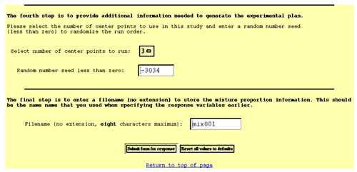
After entering the filename, the user may click on "Submit" to submit the information to COST and generate the experimental plan, or the user may click "Reset" to set all values back to their defaults (all information entered will be lost).

When "Submit" is clicked, COST processes the input and generates an experimental plan, which is displayed on the screen. The user should print this plan using the "PRINT" command in the browser. An example of a portion of an experimental plan generated by COST is shown in figure C-8.

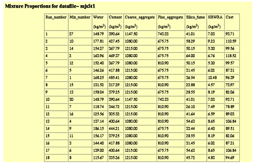
The columns in the printed table shown above correspond to the run number (the order in which the mixtures should be prepared), the mixture number (the mixture number according to standard experiment design tables), mixture proportions in terms of the mass of each component per cubic meter of concrete, and an estimated cost for each mixture based on the individual material costs provided by the user.

If the plan is not printed immediately, it can be viewed and printed at a later time by selecting "View Expt Plan" from the main menu.

C2.4 Step 3 - Run Trial Batches

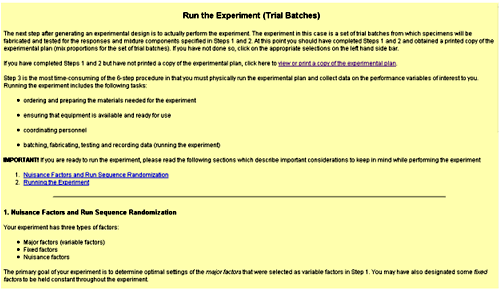
The next step after generating an experimental plan is to actually perform the experiment. The experiment in this case is a set of trial batches from which specimens will be fabricated and tested for the responses and mixture components specified in steps 1 and 2. Before running the experiment, steps 1 and 2 must be complete, and the user should have a printed copy of the experimental plan containing the mixture proportions for the set of trial batches.

When "Run Trial Batches" is selected from the main menu, the screen shown in figure C-9 appears. This screen does not require any input; rather, it provides instructions and guidelines for running the trial batches. These guidelines are also provided below.

Running the experiment is the most time-consuming task because it involves physically running the experimental plan and collecting data on the performance variables of interest. Running the experiment includes the following tasks:

• Ordering and preparing the materials needed for the experiment.
  
• Ensuring that equipment is available and ready for use.
  
• Coordinating personnel.
  
• Batching, fabricating, testing, and recording data (running the experiment).
  

The following sections describe important considerations to keep in mind while performing the experiment.

C2.4.2 Nuisance Factors and Run Sequence Randomization

There are three types of factors that affect the responses in an experiment:

• Variable factors.
  
• Fixed factors.
  
• Nuisance factors.

The primary goal of the experiment is to determine optimal settings of the variable factors specified in step 1. These are the major factors of interest. Depending on the objective, some fixed factors may have also been designated. These are less important factors that are held constant throughout the experiment.

The variable factors and fixed factors are controlled in the experiment. However, in addition to these, there are other factors that are not controlled in the experiment but which could possibly affect the experimental results. These are called nuisance factors. It is often assumed that these nuisance factors do not, or should not, have any effect, but in reality they may have an effect. Nuisance factors may include the following:

• Mid-experiment changes in instruments, equipment, environmental conditions, (temperature, pressure, humidity, etc.), measuring devices.
  
• Test procedures/protocols.
  
• Day of week.
  
• Time of day.
  
• Operators.

Nuisance factors may affect the measured test results, which would in turn affect the data analysis, and ultimately the final conclusions (i.e., the estimated values for the optimal mixture proportions).

Run sequence randomization is used to minimize the effect of nuisance factors. Experiment designs are usually generated in a "standard order" based on the settings of the factors. This order (used by COST in the data analysis) is indicated by the "mixture number" column (column 2) in the experimental plan generated by COST (figure C-8). Run sequence randomization is the general experiment design technique in which random numbers are assigned to each of the specified runs in the experiment, and these random numbers determine the order in which the experiment is to be run (the "run order" or "run sequence"). The experimental plan generated by COST is printed in run order-the first column of the experimental plan, labeled "run number," is the run order to be used for the experiment (figure C-8).

It is very important to follow the run sequence in order to minimize possible error in the experimental results caused by known or unknown nuisance factors in the experiment.

C2.4.3 Running the Experiment

The quality and accuracy of the final mixture proportion settings will depend very much on the care taken in carrying out the experiment. The following is a list of recommended practices:

• Attention to detail, consistency and proper execution in batching, mixing, fabricating, curing, testing, and recording results are essential.
• For each trial batch, use several (preferably 3 or more) specimens for each test.
• The experimental plan contains 3 or 5 center point runs. These are replicates (repeats of batches using the same settings) which can be used during the experiment as control mixes. Scheduling to allow for one control mixture per week is recommended-in this way significant week-to-week variation can be detected.
• If possible, the same operator should perform the same tasks throughout the experiment.
• Mistakes will inevitably occur even in the best laboratories, and it is important to acknowledge this and to be prepared to repeat a batch if it is suspected that an error has occurred.

C2.5 Step 4-Input Results

This section describes how to input experimental results into the COST program for analysis. The following instructions assume that steps 1, 2, and 3 have been successfully completed. Within this step, you may perform the following tasks:

• Change cost information (optional).
• review the experimental plan (optional).
• enter or edit the experimental results (data) for analysis (required).

Instructions for each of these tasks are provided below.

C2.5.1 Instructions for Changing Cost Information

Before entering the test results, you may optionally change the costs of the raw materials, if you have updated information since the project began. Please note that these updates should be made before entering in the data (test results) as described below; otherwise, the new costs will not be in effect during the analysis phase. To do so, click on the link "Update cost information." You will see a box with the caption "Datafile name". Enter the name of your datafile (no extension) in the box, and press the "Submit" button. A form entitled "COST Input Form: Update Material Costs for 'DATAFILE'" will appear. Make any necessary changes to the material costs and press "Submit" to save the changes.

If you make a mistake and would like to reset all costs to their default values, press "Reset," before pressing the "Submit" button. If you decide not to change the costs, simply press the back button on your browser to return to the previous page, or select any entry from the blue menu sidebar.

C2.5.2 Instructions for Entering/Editing Data

When you are ready to enter your data, click on "Enter or edit data in chronological (run) order." You will then see a screen entitled "COST Input Form: Testing Results (Project Filename)." Enter the project filename (with no extension) and press "Submit."

The next screen will be "COST Input Form: Test Results for 'DATAFILE.'" The first part of this form, as shown in figure C-10, allows you to make changes to the response information that you entered in step 1 (instructions are the same as for step 1 described previously). If you do not have any changes to make in the response information, simply scroll down to the second part of the form.

The second part of the form is for entry (or editing) of the experimental results, or data. The last two lines in the figure C-10 show two rows of entries for the experimental test results. The first column shows the run order for the experiment, and the second column shows the mixture number (these should correspond to the run and mixture numbers in your experimental plan). The third column is "Cost" (the first response).

IMPORTANT: Because the total cost of each mixture is calculated from the individual materials costs entered in step 1, the third column contains nonzero entries that should not be changed.

The responses requiring data entry start in the fourth column (one column per response).

• If you are entering results for the first time, these columns will contain zeros. Enter the appropriate results in these columns for each mixture.
• If you are editing a file you already created, these columns will contain nonzero values. Perform any necessary editing.

IMPORTANT: As you enter or edit your data, please check the input as you go for typographical errors and to make sure that the results are entered in the correct columns and rows.

It should be noted that some of the input values shown in figure C-10 are outside of the acceptable range specified by the lower and upper limits, as will most likely be the case for any real experiment.

When data entry is complete, you may use the "PRINT" button on your browser to print the input form.

IMPORTANT: It is highly recommended that you check the printed form for accuracy, and edit the information if necessary (to edit, simply follow the instructions in this section).

C2.6 Step 5-Analyze Data

The next step after entering the data is to analyze the results, with the ultimate goal of determining optimal mixture proportions. The analysis techniques employed by COST consist of both graphical analysis and numerical analysis (modeling). The analysis is broken down into 10 tasks, which are described in detail below.

C2.6.1 Instructions for Changing Response Information

Before analyzing the data, COST gives the user the option of changing response variable limits, weights, and function types. To do so, click on "Change response variable limits, weights, and function types." You will then be prompted for the filename. After entering the filename, press "Submit" and follow the instructions in the section "Step 1-Specify Responses."

C2.6.2 Analysis Tasks

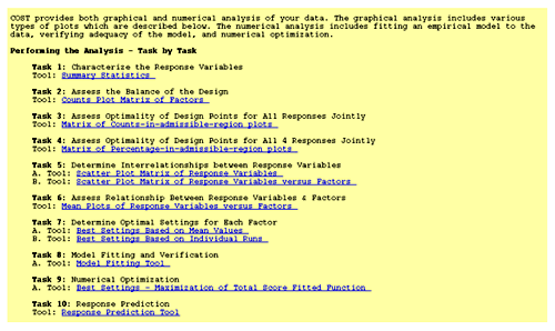
The analysis tasks are listed by the purpose of the task followed by the statistical tool used to perform the task, as shown in figure C-11. For example, the purpose of task 2 is to "Assess the Balance of the Design," and the tool used is "Counts Plot Matrix of Factors." An example and explanation of each task and tool is provided below. The output of each task is a GIF file that is generated by DATAPLOT. The GIF file contains tabular output, graphical output, or a combination of both.

C2.6.2.1 Task 1: Characterize the Response Variables

This task provides a quantitative summary of the data for each response. The result of this task is a table of descriptive statistics such as mean, range, and standard deviation for each response. An example is provided below (figure C-12).

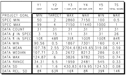
The summary statistics provided for each response and the total score (TS) are described in table C-3 (next page).

C2.6.2.2 Task 2: Assess the Balance of the Design

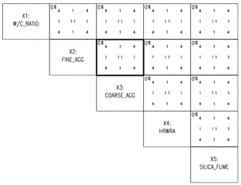
This task is a check to make sure that the design is balanced. The result of this task is a plot similar to figure C-13. Figure C-13 shows a matrix of plots showing the number of design points (experimental runs) at each setting for all combinations of two factors. For example, the highlighted box in figure C-13 shows the number of design points for the factors X2 and X3 (fine aggregate and coarse aggregate). There are nine numbers in this box, representing different settings of the factors. The lower left number indicates that there are 4 design points that have the setting "-1, -1" (in coded values) for fine aggregate and coarse aggregate. For this design every set of two factors has the same experimental layout (the sets of nine numbers in each box are the same). For any design generated by COST, this will always be the case. The percentage in the upper left corner indicates the correlation coefficient. Ideally, this will be zero. For any design generated by COST, the correlation coefficient will be zero for all sets of factors, indicating a balanced design.

Figure C-13. Output of analysis task 2 (counts plot matrix of factors)

C2.6.2.3 Task 3: Assess Optimality of Design Points for All Responses Jointly

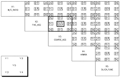
The purpose of task 3 is to see how all the responses compare to the specifications for each design point. Figure C-14 shows the output, which is a matrix of plots comparing each combination of two factors. In each large box there are nine smaller boxes, corresponding to the nine possible design settings for two factors. In each smaller box there will be between one and five numbers, depending on the number of responses being investigated. In the example below, there are five responses, and thus five numbers. The legend at the lower left of the plot indicates which number in the small box corresponds to which response (Y1, Y2, Y3, Y4, Y5). In the example below, the large box for X2 and X3 is highlighted, and the small box corresponding to settings of X2 = 0, X3 = 0 is highlighted. The numbers in the small box indicate that for these settings of X2 and X3, there was 1 response for Y1 that was within the acceptable region, there were 7 for Y2, 2 for Y3, 11 for Y4, and 11 for Y5. This information allows the user to assess how well the ranges selected for the factors allow him to meet the desired specifications. For Y1 and Y3, only a few responses met the specification. Therefore, for this set of mixture proportions, it may be difficult to optimize these responses. A new set of acceptance criteria could be defined, or different ranges for the mixture proportion factors may be needed. Other analysis tasks will give the user a sense of which direction the factors must be shifted.

C2.6.2.4 Task 4: Assess Optimality of Design Points for All Responses Jointly

Task 4 is similar to task 3 in assessing optimality of design points. For each combination of two variable settings (e.g., X2 = 0, X3 = 0), the percentage of runs falling in at least one admissible region (for all responses taken together) is shown (see figure C-15). The overall percentage for all the runs is given in the first text line below the title. In this case, it is 59 percent. The overall percentage for the number of design points meeting all "n" (in this case, 5) acceptance criteria for responses is indicated on the second line below the title. In this case, it is zero. The gray squares over the numbers in the boxes indicate the highest percentage in each box, and the triangles indicate the lowest percentage in the box. This gives a quick visual cue to the settings that are best in meeting the acceptance criteria.

C2.6.2.5 Task 5A: Determine Interrelationships between Response Variables

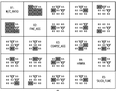
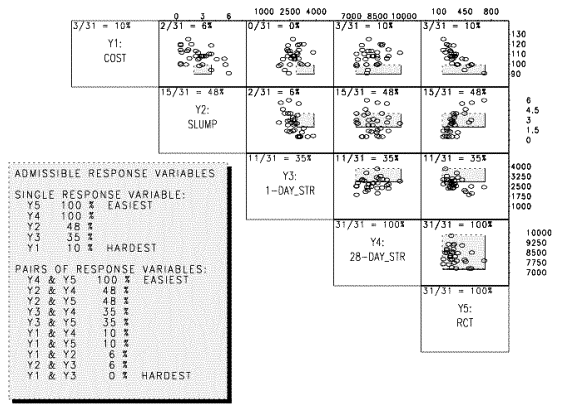
Figure C-16 shows a matrix of scatterplots showing data for each combination of two response variables (RVs). The admissible region for each pair of RVs is indicated as a gray box surrounded by dashed lines. These plots give a sense of relationships between responses and also a sense of how many points fall in the admissible region (as defined by the performance criteria set by the user) for each pair of responses. The numbers in the upper left corner of each box (e.g., 2/31 = 6 percent) indicate the number of responses falling in the admissible region. The large gray shaded box at the bottom left of the entire plot shows the relative ease or difficulty of meeting the performance criteria (i.e., falling within the admissible region) for single responses and for pairs of responses.

C2.6.2.6 Task 5B: Interrelationships between Response Variables and Factors

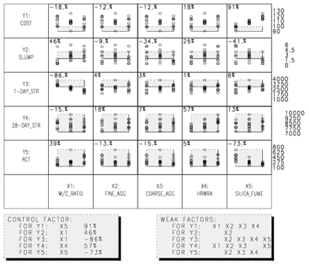
The output for this task (shown in figure C-17) shows the relationship between responses and factors. In each plot, the response values (Y axis) are shown for each factor level (X axis). The correlation coefficient (indicating the strength of the linear relationship between Y and X) is shown in the upper left corner of each plot. The stronger the linear relationship, the closer this value will be to 1 or -1 (depending on the slope). Examining these plots allows the user to assess which factors are important (controlling) for each response. The gray shaded boxes at the bottom of the plot summarize the control factors (left box, percentage indicates correlation coefficient) and the "weak" factors (right box).

C2.6.2.7 Task 6: Assess Relationship between Response Variables and Factors

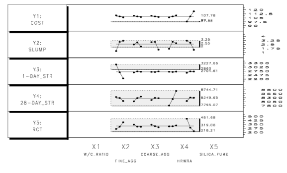
This task provides an assessment of the relationship between responses and factors by examining plots of the mean (average) values of the responses at each factor level. Figure C-18 shows the output for this task. For each response, there is a plot of the mean values at each level of each factor. The gray shaded boxes indicate the admissible region for each response. Influential factors are those that have a definite slope (for example, silica fume for response Y1, cost, or w/c ratio for Y3, 1-day strength). The steeper the slope, the more important the factor. A flat line (or nearly flat) indicates little effect of the factor (for example, fine aggregate for Y5, RCT).

C2.6.2.8 Task 7A: Best Settings for Each Factor Based on Means

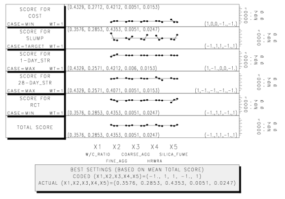
This task provides a graphical means of selecting best factor settings based on mean (average) values of "scoring functions" calculated for each response separately as well as a total score function (TS). The total score is a weighted linear combination of scores calculated for each response (the weight given to each response is defined in "Step 1-Specify Responses," as the result weight, a value ranging from zero to 1). Figure C-19 shows the output from this task.

The best settings (as coded values) are shown in parentheses on the right side of each plot. The best setting based on total score are shown in the gray box at the bottom of the plot, in both coded and actual units. As in task 6, a steep slope indicates a large influence of a particular factor on the score, while a flat slope indicates little or no influence.

C2.6.2.9 Task 7B: Best Factors Based on Individual Runs

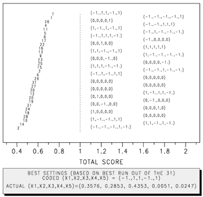
This task produces a plot (figure C-20) showing the best settings for total score (weighted linear combination of scores for individual responses) based on individual runs. The total scores for each run are calculated, sorted (lowest to highest) and plotted along the X axis. The Y axis is used to differentiate between the individual runs. Each run is indicated by its number in the experimental plan, and the coded values of each factor are provided in parentheses on the right. These values are staggered for readability. The topmost number has the highest total score.

C2.6.2.10 Task 8: Model Fitting and Verifications

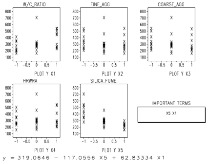
In this task, an empirical mathematical model is fitted to the data for each response, and to the total score, using the standard regression methods (least squares). A full quadratic model is fit initially, and then reduced by eliminating terms with significance level less than 0.05. When the task is selected, the response to be fitted is selected using a pull-down menu. In addition to the response variables (up to five), a model may also be fitted to total score. For a complete analysis of all responses, task 8 must be thus executed multiple times, once for total score and once for each response variable. Output similar to figure C-21 is produced for the each selected response variable. The output provides a plot for the response as a function of each factor, showing all response data for the coded values of each factor. These plots may indicate trends (see for example, the plot for silica fume in figure C-21, which indicates a downward trend in RCT test results with increasing silica fume). In addition to the plots, a summary box of the important terms in the model is provided to the right of the second row of plots, and the actual model is printed below the plots. The model is in terms of CODED values (the model can be translated to actual factor values). The model can be used to predict the response values for settings other than those used in the experiment (but within the experimental space)-a calculator for doing this is provided in task 10.

C2.6.2.11 Task 9: Numerical Optimization

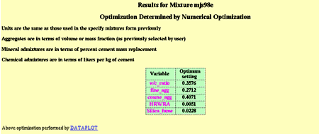
This task uses numerical optimization techniques to identify the optimal settings for total score, over the entire experimental space. This optimization is performed during the model fitting for total cost in task 8, so when task 9 is executed, the COST system simply returns a table indicating the best settings as determined by the numerical optimization, as shown in figure C-22.

C2.6.2.12 Task 10: Response Prediction

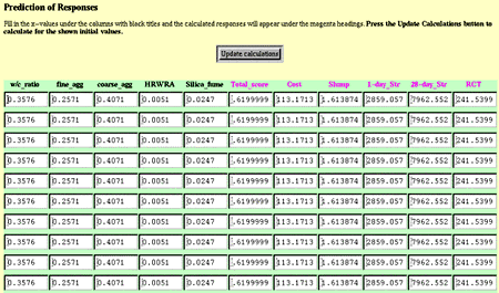
As shown in figure C-23, this task provides a calculator for predicting response values using the models from task 8. The user enters values for each factor (in terms of actual values) and the program calculates the responses and the total score. Calculations can be performed for up to 10 different combinations of factors.

C2.7 Step 6-Summarize Analysis

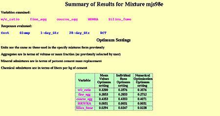
This step simply returns a table summarizing the three different optimum settings (from analysis tasks 7A, 7B, and 9) determined by the COST system, as shown in figure C-24.

SECTION 3
References

1. Box, G.E.P., Hunter, W.G., and J.S. Hunter, Statistics for Experimenters. New York, John Wiley & Sons, 1978.
   
   
2. Myers, R.H. and D.C. Montgomery, Response Surface Methodology: Process and Product Optimization Using Designed Experiments. New York, John Wiley & Sons, 1995.
   
   
3. Simon, M.J., Lagergren, E.S, and L.G. Wathne, "Optimizing High-Performance Concrete Mixtures Using Statistical Response Surface Methods." In Proceedings of the 5^th International Symposium on Utilization of High-Strength/High-Performance Concrete. Norwegian Concrete Association, Oslo, Norway, June, 1999, pp. 1311-1321.
   
   
4. Heckert, A., and J.J. Filliben, DATAPLOT Reference Manual Volume I: Commands, National Institute of Standards and Technology, 1999.