U.S. Department of Transportation
Federal Highway Administration
1200 New Jersey Avenue, SE
Washington, DC 20590
202-366-4000
Federal Highway Administration Research and Technology
Coordinating, Developing, and Delivering Highway Transportation Innovations
 |
| This report is an archived publication and may contain dated technical, contact, and link information |
|
Publication Number: FHWA-RD-03-060 |
Previous | Table of Contents | Next
2.1 Response Surface Methodology
Response surface methodology (RSM) consists of a set of statistical methods that can be used to develop improve, or optimize products [3]. RSM typically is used in situations where several factors (in the case of concrete, the proportions of individual component materials) influence one or more performance characteristics, or responses (the fresh and hardened properties of the concrete). RSM may be used to optimize one or more responses (e.g., maximize strength, minimize chloride penetration), or to meet a given set of specifications (e.g., a minimum strength specification or an allowable range of slump values). There are three general steps that comprise RSM: experiment design, modeling, and optimization. Each of these is described below.
Concrete is a mixture of several components. Water, portland cement, and fine and coarse aggregates form a basic concrete mixture. Various chemical and mineral admixtures, as well as other materials such as fibers, also may be added. For a given set of materials, the proportions of the components directly influence the properties of the concrete mixture, both fresh and hardened.
2.2 Experiment Design
Consider a concrete mixture consisting of q component materials (where q is the number of component materials). Two experiment design approaches can be applied to concrete mixture optimization: the classic mixture approach, in which the q mixture components are the variables, [7] and the mathematically independent variable (MIV) approach, in which q mixture components are transformed into q-1 independent mixture-related variables [8]. Each technique has advantages and disadvantages. In the classic mixture approach, the sum of the proportions must be 1; therefore the variables are not all independent. This allows the experimental region of interest to be defined more naturally, but the analysis of such experiments is more complicated. The MIV approach, with the variables independent, permits the use of classical factorial and response surface designs [9], but has the undesirable feature that the experimental region changes depending on how the q mixture components are reduced to q-1 independent factors.
In this report, the MIV approach is referred to as the factorial approach because factorial experiment designs form the basis of the approach. The following sections present general (nonrigorous) descriptions of each method (for a detailed discussion of these methods, see reference 3).
2.2.1 Mixture Approach
In the mixture approach, the total amount (mass or volume) of the product is fixed, and the settings of each of the q components are proportions. Because the total amount is constrained to sum to one, only q-1 of the factors (component variables) can be chosen independently.
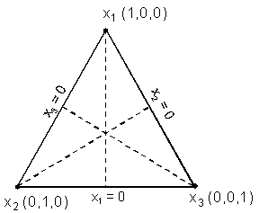
Figure 1. Example of triangular simplex region from three-component mixture experiment.
As a simple (hypothetical) example of a mixture experiment, consider concrete as a mixture of three components: water (x1), cement (x2), and aggregate (x3), where each xi represents the volume fraction of a component. Assume the coarse-to-fine aggregate ratio is held constant. The volume fractions of the components sum to one, and the region defined by this constraint is the regular triangle (or simplex) shown in figure 1. The axis for each component xi extends from the vertex it labels (xi = 1) to the midpoint of the opposite side of the triangle (xi = 0). The vertex represents the pure component. For example, the vertex labeled x1 is the pure water mixture with x1 = 1, x2 = 0, and x3 = 0, or (1,0,0). The point where the three axes intersect, with coordinates (1/3,1/3,1/3), is called the centroid.
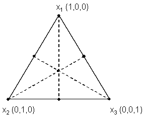
Figure 2. Simplex-centroid design for three variables
A good experiment design for studying properties over the entire region of a three-component mixture would be the simplex-centroid design shown in figure 2 (this example is included as an illustration only, since much of this region would not represent either feasible or workable concrete mixtures). The points shown in figure 2 represent mixtures included in the experiment and include all vertices, midpoints of edges, and the overall centroid.
All responses (properties) of interest would be measured for each mixture in the design and modeled as a function of the components. Typically, polynomial functions are used for modeling, but other functional forms can also be used. For three components, the linear polynomial model for a response y is:
| Equation 1: |
where the bi * are constants and e, the random error term, represents the combined effects of all variables not included in the model. For a mixture experiment,  ; therefore, the model can be reparameterized in the form:
| Equation 2: |
using ![]() . This form is called the Scheffé linear mixture polynomial [7].
. This form is called the Scheffé linear mixture polynomial [7].
Similarly, the quadratic polynomial:
| Equation 3: |
can be reparameterized as:
| Equation 4: |
using ![]() ,
,![]() , and
, and ![]() .
.
Since feasible concrete mixtures do not exist over the entire region shown in figures 1 and 2, a subregion of the full simplex containing the range of feasible mixtures must be defined by constraining the component proportions. An example of a possible subregion for the three-component example is shown in figure 3. It is defined by the following volume fraction constraints (where x1 = water, x2 = cement, x3 = aggregate):
0.15 £ x1 £ 0.25
0.10 £ x2 £ 0.20
0.60 £ x3 £ 0.70
In this case the simplex designs are usually no longer appropriate and other designs are used [3].
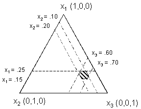
Figure 3. Example of subregion of full simplex containing range of feasible mixtures.
The advantage of the mixture approach is that the experimental region of interest is defined more naturally; however, analysis of the results can be complicated, especially if the number of components is greater than three.
2.2.2 Factorial (MIV) Approach
In the factorial approach, the q components of a mixture are reduced to q-1 independent variables using the ratio of two components as an independent variable. In the case of concrete, w/c is a natural choice for this ratio variable. For the situation with ![]() independent variables, a 2
independent variables, a 2![]() factorial design forms the backbone of the experiment. This design consists of several factors (variables) set at two different levels. As a simple example, consider a concrete mixture composed of four components: water, cement, fine aggregate, and coarse aggregate. Three independent factors, or variables, xk , that can be selected to describe this system are x1= w/c (by mass), x2 =
fine aggregate volume fraction, and x3 = coarse aggregate
volume fraction. Reasonable ranges for these variables might be:
factorial design forms the backbone of the experiment. This design consists of several factors (variables) set at two different levels. As a simple example, consider a concrete mixture composed of four components: water, cement, fine aggregate, and coarse aggregate. Three independent factors, or variables, xk , that can be selected to describe this system are x1= w/c (by mass), x2 =
fine aggregate volume fraction, and x3 = coarse aggregate
volume fraction. Reasonable ranges for these variables might be:
0.40 £ x1 £0.50
0.25 £ x2 £0.30
0.40 £ x3 £0.45
The levels for this example would be 0.40 and 0.50 for x1, 0.25 and 0.30 for x2, and 0.40 and 0.45 for x3. To simplify calculations and analysis, the actual variable ranges are usually transformed to dimensionless coded variables with a range of ±1. In this example, the actual range of 0.40 £ x1 £ 0.50 would translate to a coded range of -1 £ x1 £1. Intermediate values of x1 would translate similarly (e.g., the actual value of 0.45 would translate to a coded value of zero). The general equation used to translate from coded to uncoded is as follows:
| Equation 5: |
 |
where xactual is the uncoded value, xmin and xmax are the uncoded minimum and maximum values (corresponding to -1 and +1 coded values), and xcoded is the coded value to be translated.
Suppose that the specifications for this mixture require a slump of 75 to 150 mm and a 28-day strength of 30 MPa. These specified properties are called the responses, or dependent variables, yi, which are the performance criteria for optimizing the mixture. For concrete, the responses may be any measurable plastic or hardened properties of the mixture. Cost may also be a response.
As with the mixture approach, empirical models are fit to the data, and polynomial models (linear or quadratic) typically are used. Equation 6 illustrates the general case of the full quadratic model for k =3 independent variables:
| Equation 6: |
In equation 6, the ten coefficients are represented by the bk and e is a random error term representing the combined effects of variables not included in the model. The interaction terms (xixj) and the quadratic terms (xi2) account for curvature in the response surface.
The central composite design(CCD), an augmented factorial design, is commonly used in product optimization. A complete CCD experiment design allows estimation of a full quadratic model for each response. A schematic layout of a CCD for k = 3 independent variables is shown in figure 4. The design consists of 2k (in this case, 8) factorial points (filled circles in figure 4) representing all combinations of coded values xk = ±1, 2*k (in this case, 6) axial points (hollow circles in figure 4) at a distance ±a from the origin, and at least 3 center points (hatched circle in figure 4) with coded values of zero for each xk. The value of a usually is chosen to make the
design rotatable[1], but there are sometimes valid reasons to select other values [3].
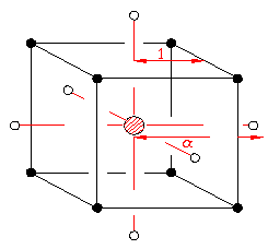
Figure 4: Schematic of a composite design for three factors
In the absence of curvature, a model with only linear terms would be sufficient, and the factorial portion of the CCD is a valid design by itself in that case. However, the presence or absence of significant curvature often is not known with certainty at the start. An advantage of the CCD over the mixture approach is that the CCD can be run sequentially in two blocks. The first block would consist of the factorial points (all combinations of xi = ±1) and some center points (at least 3), and the second block would consist of the axial points (points along each axis at distance a from the origin) and additional center points (at least 2). This approach allows analysis of the factorial portion before the axial portion is run. If curvature is insignificant based on the factorial portion, the additional runs are not necessary.
As shown in table 1, the number of coefficients in the quadratic model increases with k, and the number of trial batches required using a CCD begins to increase significantly for k> 5.
Table 1. Number of runs required for CCD experiment for k = 2 to 5 factors
| k | Factorial | Axial | Center* | Total |
|---|---|---|---|---|
| 2 | 4 | 4 | 5 | 13 |
| 3 | 8 | 6 | 5 | 19 |
| 4 | 16 | 8 | 5 | 29 |
| 5 | 16** 16** | 10 | 5 | 31 |
| *assumes 3 CP for factorial portion and 2 CP for axial portion **for k=5, a half-fraction of the full factorial is sufficient to estimate all linear terms and 2-factor interactions without confounding. Thus, 25-1 or 16 factorial points are usually sufficient | ||||
Therefore, using a CCD to optimize a concrete mixture of more than six components may be uneconomical. In such cases, one could identify the most important factors and limit them to five or fewer. For example, if the cementitious materials and chemical admixtures were the most important components, they would be varied, while the amounts of coarse and fine aggregate would be held constant.
Laboratory experiments were conducted using the mixture and factorial approaches to see if one was more appropriate for concrete mixture optimization. The experiments are described in chapters 3 and 4. The adaptability of each method for use as an interactive, Web-based program was also considered in developing the COST software, described in chapter 5.
2.3 Model Fitting and Validation
The polynomial models described in sections 2.2.1 and 2.2.2 are fit to data using analysis of variance (ANOVA) and least squares techniques [9]. Many statistical software packages have the capability to perform these analyses and fits. Once a model has been fit, it is important to verify the adequacy of the chosen model quantitatively and graphically.
Although the models (polynomials) are slightly different for the classical mixture approach and the factorial approach, many of the steps involved in model selection and fitting are the same. The first step in each case is to perform ANOVA to select the appropriate type of model (linear, quadratic, etc.). Sequential F-tests are performed, starting with a linear model and adding terms (quadratic, and higher if appropriate). Under the "Source" column of the ANOVA table, the line labeled "Linear" indicates the significance of adding linear terms, and the line labeled "Quadratic" indicates the significance of adding quadratic terms. The column labeled "DF" shows the degrees of freedom for each source. The F-statistic is calculated for each type of model, and the highest order model with significant terms normally would be chosen. Significance is judged by determining if the probability that the F-statistic calculated from the data exceeds a theoretical value. The probability decreases as the value of the F-statistic increases. If this probability is less than 0.05 (typically, although other levels of significance could be used), the terms are significant and their inclusion improves the model. An example of an ANOVA table for sequential model sum of squares is shown in table 2.
Table 2. Example of ANOVA sequential model sum of squares
| Source | Sum of Squares | DF | Mean Square | F Value | Prob > F |
|---|---|---|---|---|---|
| Mean | 329.27 | 1 | 329.27 | - | - |
| Linear | 96.94 | 5 | 19.39 | 45.64 | < 0.0001 |
| Quadratic | 6.36 | 15 | 0.42 | 1.00 | 0.5017 |
| Special Cubic (aliased) | 3.35 | 7 | 0.48 | 1.26 | 0.3727 |
| Cubic (aliased) | 0.00 | 0 | - | - | - |
| Residual | 3.03 | 8 | 0.38 | - | - |
| Total | 438.95 | 36 | 12.19 | - | - |
In this example, the linear model is the highest order model with significant terms (Prob > F is less than 0.05); therefore, it would be the recommended model for this data. Typically, the selected model will be the highest order polynomial where additional terms are significant and the model is not aliased.
Once the type of model (e.g., linear, quadratic, etc.) is selected, the second step is to perform a lack-of-fit test, also using ANOVA, to compare the residual error to the pure error from replication. Table 3 is an example of ANOVA for lack of fit. If residual error significantly exceeds pure error, the model will show significant lack of fit, and another model may be more appropriate.
The desired result in a lack-of-fit test is that the model selected in step 1 will not show significant lack of fit (i.e., the F test will be insignificant). If the "Prob > F" value is less than the desired significance level (often .05), this indicates significant lack of fit.
Several summary statistics can be calculated for a model and used to compare models or verify model adequacy. These statistics include root mean square error (RMSE), adjusted r2, predicted r2, and prediction error sum of squares (PRESS). The RMSE is the square root of the mean square error, and is considered to be the standard deviation associated with experimental error. The adjusted r2 is a measure of the amount of variation about the mean explained by the model, adjusted for the number of parameters in the model [2].
Table 3. Example of ANOVA lack-of-fit test
| Source | Sum of Squares | DF | Mean Square | F Value | Prob > F |
|---|---|---|---|---|---|
| Linear | 6271.93 | 22 | 285.09 | 1.17 | 0.4335 |
| Quadratic | 2164.86 | 7 | 309.27 | 1.27 | 0.3703 |
| Special Cubic (aliased) | 0.00 | 0 | - | - | - |
| Cubic (aliased) | 0.00 | 0 | - | - | - |
| Pure Error | 1950.91 | 8 | 243.86 | - | - |
The predicted r2 measures the amount of variation in new data explained by the model. PRESS measures how well the model fits each point in the design. To calculate PRESS, the model is used to estimate each point using all of the design points except the one being estimated. PRESS is the sum of the squared differences between the estimated values and the actual values over all the points. A good model will have a low RMSE, a large predicted r2, and a low PRESS.
After a model is selected, standard linear regression techniques (least squares) are used to fit the model to the data. ANOVA is performed and an overall F-test and lack-of-fit test confirm the applicability of the model. Summary statistics (r2, adjusted r2, PRESS, etc.) and the standard error for each model coefficient also are calculated.
For the factorial approach, an iterative model fitting process was used in this research. First, a full quadratic (or linear, if applicable) model is assumed, and significance tests (t-tests) are performed on each model coefficient. Insignificant terms are removed and the fitting process is repeated using a partial quadratic (or linear, if applicable) model. The significance tests are repeated and insignificant terms, if any, are removed. The process is repeated until there are no insignificant terms. At this point, if the model contains two-factor interaction or quadratic terms, it is checked for hierarchy. Hierarchical terms are linear terms that may be insignificant by themselves but are part of significant higher order terms. For example, x1and x3 are hierarchical terms of x1x3, a two-factor interaction term. If x1x3 is a significant term in the model, x1 and x3 are usually included in the model to maintain hierarchy. A hierarchical model allows for conversion of models between different sets of units (for a model involving temperature, conversion from F to C, for example).
Table 4 shows an ANOVA table for a selected model from a factorial experiment. Using the iterative approach, a reduced quadratic model was fit to the data. Note that terms B, C, and E are not significant ("Prob > F" >.05) but were added back into the model to make it hierarchical.
Table 4. Example of ANOVA model fitting for 1-day strength
| Source | Sum of Squares | DF | Mean Square | F Value | Prob > F |
|---|---|---|---|---|---|
| Model | 240.87 | 8 | 30.11 | 27.76 | < 0.0001 |
| A | 213.26 | 1 | 213.26 | 196.66 | < 0.0001 |
| B | 0.48 | 1 | 0.48 | 0.45 | 0.5113 |
| C | 0.04 | 1 | 0.04 | 0.04 | 0.8433 |
| E | 2.06 | 1 | 2.06 | 1.90 | 0.1819 |
| A2 | 6.20 | 1 | 6.20 | 5.72 | 0.0257 |
| AC | 5.15 | 1 | 5.15 | 4.75 | 0.0404 |
| AE | 7.16 | 1 | 7.16 | 6.60 | 0.0175 |
| BC | 6.51 | 1 | 6.51 | 6.00 | 0.0227 |
| Residual | 23.86 | 22 | 1.08 | - | - |
| Lack of fit | 19.08 | 18 | 1.06 | 0.89 | 0.6248 |
| Pure error | 4.78 | 4 | 1.19 | - | - |
| Corr. total | 264.72 | 30 |
Once the model fitting is performed, the next step is residual analysis to validate the assumptions used in the ANOVA. This analysis includes calculating case statistics to identify outliers and examining diagnostic plots such as normal probability plots and residual plots. If these analyses are satisfactory, the model is considered adequate, and response surface (contour) plots can be generated. Contour plots can be used for interpretation and optimization.
2.4 Optimization
When appropriate models have been established, several responses can be optimized simultaneously. Optimization may be performed using mathematical (numerical) or graphical (contour plot) approaches. Generally, graphical optimization is limited to cases in which there are only a few responses.
Numerical optimization requires defining an objective function (called a desirability or score function) that reflects the levels of each response in terms of minimum (zero) to maximum (one) desirability. One approach uses the geometric mean of the desirability functions for each individual response, where n is the number of responses to be optimized [10]:
| Equation 7: |
Another approach is to use a weighted average of desirability functions:
| Equation 8: |
where n is the number of responses and wi are weighting functions ranging from 0 to 1.
Several types of desirability functions can be defined. Common types of desirability functions are shown in figure 5.
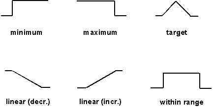
Figure 5. Examples of desirability functions
These functions can also be expressed mathematically as well. For example, a linear desirability function where minimum is best would be expressed as:
| Equation 9: |
 |
for the range Ai ![]() Yi
Yi
![]() Bi and with wi = 1.
Bi and with wi = 1.
Once the desirability functions (and weights, if used) are defined for each response, optimization may proceed.
As an alternative to rigorous numerical methods, desirability can be evaluated by superimposing a grid of points at equal spacing over the experimental region and evaluating desirability at each point. The point(s) of maximum desirability can be found by sorting the results or by creating contour plots of desirability over the grid area.
1 If a design is rotatable, predicted values should have equal variances at locations equidistant from the origin.
2 The adjusted r2 differs from the "standard" r2, which is not adjusted for the number of parameters. The standard r2 can be made larger by adding more parameters to the model. This does not necessarily mean the model with more parameters is a better model.