U.S. Department of Transportation
Federal Highway Administration
1200 New Jersey Avenue, SE
Washington, DC 20590
202-366-4000
Federal Highway Administration Research and Technology
Coordinating, Developing, and Delivering Highway Transportation Innovations
 |
| This report is an archived publication and may contain dated technical, contact, and link information |
|
Publication Number: FHWA-RD-03-060 |
Previous | Table of Contents | Next
4.1 Introduction
This chapter describes the application of factorial experiment design to the problem of concrete mixture optimization. In a mixture, the total amount (mass or volume) of the product is fixed, and the settings of each of the q components are proportions. Because the total amount is constrained to sum to one, the component variables are not independent. However, the q components can be reduced to q-1 mathematically independent variables using the ratio of two components as an independent variable [8]. In the case of concrete, w/c is a natural choice for this ratio variable. If this strategy is adopted, a factorial approach may be applied.
4.2 Selection of Materials, Proportions, and Constraints
The materials used in this experiment were identical to those used in the mixture experiment (chapter 3): Type I cement, tap water, #57 crushed limestone, natural sand, silica fume (slurry), and naphthalene-sulfonate-based HRWRA. The six components were reduced to five independent variables: x1 = w/c (by mass), x2 = fine aggregate volume fraction, x3 = coarse aggregate volume fraction, x4 = HRWRA volume fraction, x5 = silica fume volume fraction.
The volume fraction ranges for coarse aggregate, fine aggregate, HRWRA, and silica fume were the same as used in the mixture experiment. The range of w/c (by volume) was calculated from the volume fraction limits of the mixture experiment. The lower limit of w/c was 0.16 ÷ 0.15 = 1.067, and the upper limit was 0.185 ÷0.13 = 1.423. These limits were equated to coded limits of -1.5 to +1.5 to give the most similar experimental region to that of the mixture experiment. Table 9 shows the settings of each variable corresponding to coded values of -1 and +1.
Table 9. Variable settings corresponding to coded values (factorial experiment)
| Variable | ID | Low Setting (coded value = -1) | High Setting (coded value = 1) |
|---|---|---|---|
| w/c ratio | x1 | 1.1263 (@ 0.36 by mass) | 1.3637 (@ 0.43 by mass) |
Fine aggregate | x2 | 0.2571 | 0.2853 |
Coarse aggregate | x3 | 0.4071 | 0.4353 |
HRWRA | x4 | 0.0051 | 0.0069 |
Silica fume | x5 | 0.0153 | 0.0247 |
For the aggregates, HRWRA, and silica fume, volume fractions were converted to batch masses (batch volume for HRWRA) based on total batch size and material properties. The batch masses of water and cement were calculated by constraining the sum of volume fractions of all six components to sum to one. This gives two equations in two unknowns (the other equation being the w/c expressed volumetrically) that can be solved for volume fraction of water and volume fraction of cement. Entrapped air was ignored in these calculations, although in practice it will affect yield calculations and an overall adjustment to the mixture proportions may be necessary for proper yield.
The performance criteria for the mix were as follows: slump between 50 and 100 mm, 1-day strength greater than 22 MPa, 28-day strength greater than 51 MPa, and charge passed in the RCT less than 700 coulombs. These are the same performance criteria used for the mixture experiment, except that the 1-day and 28-day strengths were rounded to 22 and 51 MPa (from 22.06 and 51.02 MPa used in the mixture experiment)1.
4.3 Experiment Design Details
A central composite design (see chapter 2) was chosen for this experiment. The actual values for each variable (expressed in terms of volume fraction) corresponding to the coded levels ±1 are shown in table 10. A commercially available software package for experiment design and analysis was used to plan the experiment. Thirty-one batches were planned in two nearly orthogonal blocks. The first block consisted of a half-fraction of 16 factorial points2 and 3 center points, and the second block consisted of 10 axial points and 2 center points. A total of five center points was chosen to allow use of the center point mixes as statistical control mixes to assess week-to-week variation, if any, over the five weeks of mixing (in addition to the use of center points as replicates to estimate pure error). The run order within each block was randomized to reduce the effect of uncontrolled variables. Center point runs were placed first and last (based on the total number of runs) with the remainder equally spaced, resulting in three center points in the factorial block and two center points in the axial block. The mixture proportions for each batch are shown in table 10.
One batch (run 3) was repeated at the end of the experiment because of suspiciously low strength values. A center point batch was included with the repeat to check statistical control. The results of the repeated batch were used in subsequent analyses.
4.4 Specimen Fabrication and Testing
The materials used in this study included a portland cement conforming to ASTM specification C150-94 Type I/II, a #57 crushed limestone coarse aggregate meeting grading requirements of AASHTO M43, a natural sand fine aggregate, silica fume (in slurry form), a naphthalene-sulfonate based HRWRA (ASTM C494-98 Type F/G), and municipal tap water. Thirty-one batches of concrete, each approximately 0.04 m3 in volume, were prepared over a 6-week period. Each batch was prepared in accordance with mixing procedures set forth in ASTM C192-95.
Table 10. Mixture proportions (per m3) for factorial experiment
| Batch (run) | w/c | Fine Agg (kg) | Coarse Agg (kg) | HRWRA (L) | Silica Fume (kg) | Cement (kg) | Water (kg) |
|---|---|---|---|---|---|---|---|
| 1 | 0.36 | 755.7 | 1098.7 | 6.90 | 54.3 | 408.7 | 146.1 |
| 2 | 0.36 | 755.7 | 1174.8 | 5.10 | 54.3 | 369.6 | 132.2 |
| 3 | 0.40 | 718.4 | 1136.8 | 6.00 | 44.0 | 394.9 | 156.1 |
| 4 | 0.40 | 718.4 | 1136.8 | 6.00 | 44.0 | 394.9 | 156.1 |
| 5 | 0.43 | 681.0 | 1098.7 | 6.90 | 54.3 | 405.2 | 175.4 |
| 6 | 0.43 | 755.7 | 1098.7 | 5.10 | 54.3 | 370.1 | 160.2 |
| 7 | 0.43 | 755.7 | 1098.7 | 6.90 | 33.6 | 380.2 | 164.6 |
| 8 | 0.43 | 681.0 | 1098.7 | 5.10 | 33.6 | 420.1 | 181.9 |
| 9 | 0.36 | 681.0 | 1098.7 | 5.10 | 54.3 | 453.1 | 162.0 |
| 10 | 0.40 | 718.4 | 1136.8 | 6.00 | 44.0 | 394.9 | 156.1 |
| 11 | 0.43 | 755.7 | 1174.8 | 5.10 | 33.6 | 345.0 | 149.4 |
| 12 | 0.36 | 681.0 | 1098.7 | 6.90 | 33.6 | 464.4 | 166.0 |
| 13 | 0.43 | 681.0 | 1174.8 | 5.10 | 54.3 | 370.1 | 160.2 |
| 14 | 0.36 | 755.7 | 1098.7 | 5.10 | 33.6 | 425.3 | 152.1 |
| 15 | 0.43 | 681.0 | 1174.8 | 6.90 | 33.6 | 380.2 | 164.6 |
| 16 | 0.36 | 755.7 | 1174.8 | 6.90 | 33.6 | 380.9 | 136.2 |
| 17 | 0.36 | 681.0 | 1174.8 | 6.90 | 54.3 | 408.7 | 146.1 |
| 18 | 0.36 | 681.0 | 1174.8 | 5.10 | 33.6 | 425.3 | 152.1 |
| 19 | 0.43 | 755.7 | 1174.8 | 6.90 | 54.3 | 330.1 | 142.9 |
| 20 | 0.40 | 718.4 | 1212.9 | 6.00 | 44.0 | 355.4 | 140.5 |
| 21 | 0.47 | 718.4 | 1136.8 | 6.00 | 44.0 | 357.2 | 168.1 |
| 22 | 0.40 | 793.1 | 1136.8 | 6.00 | 44.0 | 355.4 | 140.5 |
| 23 | 0.40 | 718.4 | 1136.8 | 7.80 | 44.0 | 392.4 | 155.1 |
| 24 | 0.40 | 718.4 | 1136.8 | 6.00 | 44.0 | 394.9 | 156.1 |
| 25 | 0.32 | 718.4 | 1136.8 | 6.00 | 44.0 | 441.7 | 141.3 |
| 26 | 0.40 | 718.4 | 1136.8 | 4.20 | 44.0 | 397.5 | 157.1 |
| 27 | 0.40 | 718.4 | 1136.8 | 6.00 | 23.3 | 408.1 | 161.3 |
| 28 | 0.40 | 718.4 | 1060.6 | 6.00 | 44.0 | 434.5 | 171.7 |
| 29 | 0.40 | 718.4 | 1136.8 | 6.00 | 44.0 | 394.9 | 156.1 |
| 30 | 0.40 | 718.4 | 1136.8 | 6.00 | 64.7 | 381.8 | 150.9 |
| 31 | 0.40 | 643.7 | 1136.8 | 6.00 | 44.0 | 434.5 | 171.7 |
Precautions were taken to compensate for mortar retained by the mixer, by "buttering" the mixer prior to preparing each batch. The concrete was mixed using a rotating-drum machine mixer with a 0.17 m3 mixing capacity.
Each batch included sufficient concrete for 2 slump tests, 1 unit weight and air content test (ASTM C138 and ASTM C231), and 10 100 mm x 200 mm cylinders. All cylinders were fabricated in accordance with ASTM C192, except that external vibration (a vibrating table) was utilized for consolidation in lieu of rodding when slump was less than 50 mm. Immediately following casting, the cylinders were covered with plastic and left in the molds at room temperature for 24 ± 8 hours, after which they were removed from the molds and moist cured at 23 ± 2 ºC until testing. Specimens were tested for compressive strength in accordance with ASTM C39 at the ages of 1 and 28 days. In most cases, three cylinders were tested at each age, however, where anomalies in either specimen condition or test results were evident, a fourth or fifth specimen may have been tested. Prior to compression testing, the ends of each cylinder were ground plane and parallel in accordance with ASTM C39 tolerances. Three of the remaining cylinders from each batch were used for the RCT testing. Testing was performed according to ASTM C1202, except that the 50 mm test specimens were cut from the middle of each cylinder instead of from the top. All RCTs were performed at an age of 42 days from casting.
4.5 Results and Analysis
4.5.1 Responses
The average values for slump, 1-day strength, 28-day strength, and charge passed (RCT) for each batch are shown in table 11, along with the estimated cost (dollars per cubic meter) of the concrete mixture. The costs were calculated from the mixture proportions for each batch, based on approximate component costs obtained from a local (mid-Atlantic) ready-mix concrete producer. Each response was analyzed individually by examining summary plots of the data (scatterplots and means plots), fitting a model using ANOVA and least-squares methods, validating the model by examining the residuals for trends and outliers, and interpreting the model graphically. A detailed discussion of the analysis procedure for 1-day strength is presented in the following 2 sections. The analyses for the other responses were performed in a similar manner. The models for the other responses are reported in section 4.5.4.
4.5.2 Exploratory Data Analysis for 1-Day Strength
One advantage of the factorial approach is the ability to perform an initial assessment of the data using graphical techniques such as raw data plots, means plots, scatterplots, and cube plots. These techniques are illustrated in figures 12-15 (for complete sets of plots for each response, see appendix B). A raw data plot of 1-day strength is shown in figure 12. This plot illustrates the variation in the response (1-day strength) over time, for each run. The control batch results, shown as hollow squares, give an indication of consistency over time. In this case, the control results are all about equal, indicating no time-related effects. Raw data plots are also helpful in identifying suspect data values, which may result from (for example) errors in data recording or data entry, equipment malfunction, or poor specimen fabrication.
Table 11. Test results and costs (factorial experiment)
| Batch (run) | Slump (mm) | 1 Day (MPa) | 28 Day (MPa) | RCT (coul) | Cost ($/m3) |
|---|---|---|---|---|---|
| 1 | 73 | 16.3 | 58.5 | 286 | 119.77 |
| 2 | 44 | 22.6 | 59.8 | 209 | 113.93 |
| 3 | 13 | 20.8 | 52.6 | 160 | 107.71 |
| 4 | 102 | 16.5 | 60.4 | 296 | 107.71 |
| 5 | 57 | 16.4 | 55.0 | 257 | 118.49 |
| 6 | 143 | 13.6 | 58.6 | 541 | 112.96 |
| 7 | 67 | 12.9 | 50.4 | 502 | 99.21 |
| 8 | 13 | 20.3 | 52.4 | 234 | 97.83 |
| 9 | 86 | 18.4 | 63.0 | 305 | 118.75 |
| 10 | 102 | 15.2 | 54.8 | 445 | 107.71 |
| 11 | 140 | 20.7 | 62.3 | 412 | 93.70 |
| 12 | 32 | 17.1 | 56.2 | 252 | 105.09 |
| 13 | 13 | 24.2 | 54.2 | 341 | 112.98 |
| 14 | 76 | 17.2 | 50.3 | 534 | 99.24 |
| 15 | 13 | 21.3 | 59.2 | 278 | 99.23 |
| 16 | 13 | 20.9 | 60.5 | 206 | 100.27 |
| 17 | 57 | 18.8 | 56.6 | 315 | 119.78 |
| 18 | 29 | 21.9 | 58.3 | 355 | 99.26 |
| 19 | 35 | 16.1 | 62.9 | 230 | 114.36 |
| 20 | 38 | 19.0 | 58.6 | 211 | 105.49 |
| 21 | 117 | 14.5 | 53.9 | 458 | 104.63 |
| 22 | 67 | 17.8 | 62.4 | 294 | 105.48 |
| 23 | 64 | 19.9 | 67.5 | 268 | 111.16 |
| 24 | 16 | 26.4 | 58.5 | 189 | 107.71 |
| 25 | 79 | 19.0 | 57.0 | 257 | 111.52 |
| 26 | 64 | 19.1 | 50.9 | 273 | 104.27 |
| 27 | 152 | 16.8 | 54.4 | 705 | 90.56 |
| 28 | 95 | 20.2 | 53.3 | 307 | 109.93 |
| 29 | 35 | 18.4 | 55.2 | 162 | 107.71 |
| 30 | 102 | 17.4 | 50.4 | 332 | 124.87 |
| 31 | 76 | 18.4 | 55.2 | 277 | 109.95 |
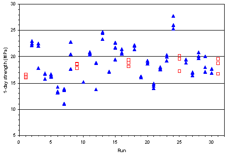
Figure 12. Raw data plot for 1-day strength (factorial experiment)
Figure 13 is a scatterplot showing the effects of varying one factor (w/c) on the 1-day strength. In this case, as expected, the 1-day strength decreases with increasing w/c.
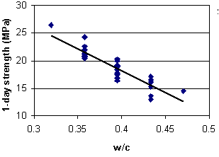
Figure 13. Scatterplot showing effect of w/c on 1-day strength (factorial experiment)
Figure 14 shows a means plot for 1-day strength. The means plot allows comparison of the effects of each factor. In this experiment, 1-day strength was clearly influenced by w/c. Other factors appear to have had little effect.
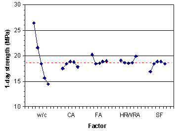
Figure 14. Means plot for 1-day strength (factorial experiment)
Finally, figure 15 shows a cube plot of 1-day strength with respect to three factors (w/c, fine aggregate, and coarse aggregate). A cube plot is a convenient means of assessing quantitative effects of three factors on a response.
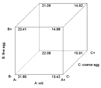
Figure 15: Example of cube plot of factorial points
4.5.3 Model Fitting and Validation for 1-Day Strength
After assessing the data graphically, the second step in analysis is to estimate an appropriate model for each response. As with the mixture approach, ANOVA and least-squares regression techniques are used. The first step is to use ANOVA to determine the appropriate type of model (e.g., linear, quadratic). An ANOVA table for sequential model sum of squares, shown in table 12, suggests that both linear and quadratic terms are significant. A lack-of-fit ANOVA table (table 13) suggests that a quadratic model has insignificant lack-of-fit ("Prob > F" = 0.8339).
Table 12. Sequential model sum of squares for 1-day strength (factorial experiment)
| Source | Sum of Squares | DF | Mean Square | F Value | Prob > F |
|---|---|---|---|---|---|
| Mean | 10780.54 | 1 | 10780.54 | - | - |
| Linear | 215.97 | 5 | 43.19 | 22.15 | < 0.0001 |
| 2FI | 27.35 | 10 | 2.73 | 1.92 | 0.1236 |
| Quadratic | 13.60 | 5 | 2.72 | 3.48 | 0.0441 |
| Cubic (aliased) | 1.86 | 5 | 0.37 | 0.31 | 0.8865 |
| Residual | 5.95 | 5 | 1.19 | - | - |
| Total | 11045.26 | 31 | 356.30 | - | - |
Table 13. Lack-of-fit test for 1-day strength (factorial experiment)
| Source | Sum of Squares | DF | Mean Square | F Value | Prob > F |
|---|---|---|---|---|---|
| Linear | 43.98 | 21 | 2.09 | 1.75 | 0.3129 |
| 2FI | 16.63 | 11 | 1.51 | 1.27 | 0.4444 |
| Quadratic | 3.03 | 6 | 0.51 | 0.42 | 0.8339 |
| Cubic (aliased) | 1.18 | 1 | 1.18 | 0.98 | 0.3772 |
| Pure Error | 4.78 | 4 | 1.19 |
When a central composite design is used, the full quadratic model can be estimated, but often some of the terms are not significant. The following procedure3 was used to identify an appropriate reduced quadratic model:
1) Fit the full quadratic model and for each coefficient, calculate the t-statistic for the null hypothesis that the coefficient is equal to zero.
2) Perform the regression again with a partial model containing only those terms that are statistically significant (i.e., those terms that had a t-statistic greater than that for the chosen significance level, in this case 0.05). Calculate the t-statistics again and drop any terms which are not significant.
3) Repeat step 2 until the partial model contains only significant terms.
4) Add first-order terms required to make the model hierarchical. Hierarchical polynomial models make sense under linear transformations such as changing units of temperature from Celsius to Fahrenheit [11]. All second-order terms that appear in the model must have corresponding first-order terms included in order to make the model hierarchical.
The ANOVA for the final hierarchical model (with the hierarchical terms shaded) is shown in table 14.
Table 14. ANOVA for 1-day strength model (factorial experiment)
| Source | Sum of Squares | DF | Mean Square | F Value | Prob > F |
|---|---|---|---|---|---|
| Model | 240.87 | 8 | 30.11 | 27.76 | < 0.0001 |
| A | 213.26 | 1 | 213.26 | 196.66 | < 0.0001 |
| B | 0.48 | 1 | 0.48 | 0.45 | 0.5113 |
| C | 0.04 | 1 | 0.04 | 0.04 | 0.8433 |
| E | 2.06 | 1 | 2.06 | 1.90 | 0.1819 |
| A2 | 6.20 | 1 | 6.20 | 5.72 | 0.0257 |
| AC | 5.15 | 1 | 5.15 | 4.75 | 0.0404 |
| AE | 7.16 | 1 | 7.16 | 6.60 | 0.0175 |
| BC | 6.51 | 1 | 6.51 | 6.00 | 0.0227 |
| Residual | 23.86 | 22 | 1.08 | - | - |
| Lack of fit | 19.08 | 18 | 1.06 | 0.89 | 0.6248 |
| Pure error | 4.78 | 4 | 1.19 | - | - |
| Corr. total | 264.72 | 30 | - | - | - |
For one-day strength, y2, the fitted model was:
| Equation 17: |
 |
The adequacy of each fitted model was validated quantitatively by calculating statistical measures such as residual standard deviation and PRESS, and graphically by examining residual plots. The residual standard deviation, s, for this model is 0.99 MPa. A value of s near the repeatibility value (replicate standard deviation calculated from center points) is an indication of an adequately fitting model. For this experiment, the repeatibility value is 1.04 MPa, which is close to s. The PRESS statistic (see page 12) is a measure of how well the model fits each point in the design (the smaller the PRESS statistic, the better the fit). PRESS and some other quantitative indicators of model adequacy are shown in table 15.
Table 15. Summary statistics for 1-day strength model (factorial experiment)
| Std. dev. | 1.04 |
| Mean | 18.65 |
| C.V. | 5.58 |
| PRESS | 45.16 |
| R-squared | 0.9099 |
| Adjusted R-squared | 0.8771 |
| Predicted R-squared | 0.8294 |
The residuals are the deviations of the observed data values from the fitted values, xI , and are estimates of the error terms ei in the model. The ei are assumed to be random and normally distributed with mean equal to zero and constant standard deviation. A normal probability plot of the residuals (shown in figure 16) is used to assess the validity of this assumption. If the error terms follow a normal distribution, they will fall on a straight line on the normal probability plot. Because they are estimates of the error terms, the residuals should exhibit similar properties.
If the assumptions are valid, plots of the residuals versus run sequence, predicted values, and other independent variables should be random and structureless. If structure remains in the residuals, residual plots may suggest modifications to the model that will remove the structure.
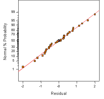
Figure 16: Example of a normal probability plot for model validation
Figure 17 shows a plot of residuals versus run sequence for 1-day strength. The plot shows no significant structure to the residuals.
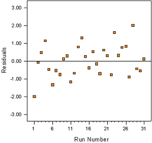
Figure 17. Example of a resident plot (residuals vs. run) for model validation
4.5.4 Models for Other Responses
Using the same procedure described above for 1-day strength, the following models were fit to slump (x1), 28-day strength (x3), and 42-day RCT (x4) results:
| Equation 18: |
 |
| Equation 19: |
| Equation 20: |
4.6 Optimization
The objective of optimization may be to find the "best settings" (settings which maximize or minimize a particular response or responses) or to meet a set of specifications. In either case, optimization usually involves considering several responses simultaneously. The same optimization strategy that was used in the classical mixture approach can be used for a factorial approach (see chapter 3).
4.6.1 Graphical Optimization
For three or fewer responses, contour plots can be useful in identifying optimum settings. Individual contour plots can be used to identify best settings for each response. Figure 18 shows a contour plot of 28-day strength as a function of w/c and silica fume with HRWRA at its middle setting. Figure 19 shows the same plot but with HRWRA at the high setting. These plots illustrate that the highest strength is reached at the high level of HRWRA coupled with the low levels of w/c and silica fume.
Contour plots can also be overlaid with the constraints for each response defining a subarea of settings that meet the response criteria. For example, figure 20 shows all settings meeting the following criteria: RCT < 700 and slump equal 50 to 100 mm. The white area in the plot indicates the settings meeting the criteria. The gray area on the plot shows the region of settings that do not meet the constraints simultaneously. Figure 21 shows the same plot with the added constraint that 28-day strength > 51 MPa. As constraints are added, the feasible region usually gets smaller. In some situations, no settings will meet all of the criteria.
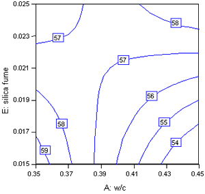
Figure 18. 28-day strength in w/c and silica fume (HRWRA) at middle setting)
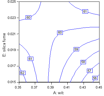
Figure 19. 28-day strength in w/c and silica fume (HRWRA at high setting)
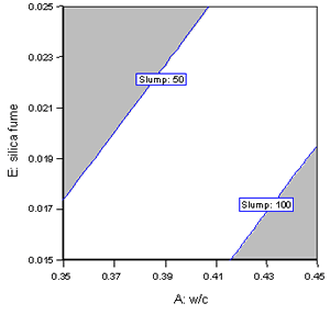
Figure 20. Overlay plot for RCT <700 and slump = 50-100 mm
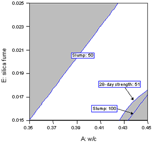
Figure 21. Overlay plot for RCT < 700, slump = 50 - 100 mm, and 28-day strength > 51 MPa
4.6.2 Numerical OptimizationFor more than three responses considered simultaneously, numerical optimization is often more practical than graphical optimization. The numerical optimization technique using desirability functions described in chapter 2 and used in the classical mixture experiment (chapter 3) can also be applied to the factorial experiment. Desirability functions for this experiment are similar to those used in the mixture experiment, except that in some cases (e.g, cost) the endpoint values are different. The desirability functions are shown in figure 22.
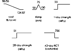
Figure 22. Desirability functions for factorial experiment
Numerical optimization gave the following best settings for this concrete mixture: w/c = 0.367 (by mass), fine aggregate volume fraction = 0.285, coarse aggregate volume fraction = 0.408, HRWRA volume fraction = 0.0061, and silica fume volume fraction = 0.0153. The predicted response values and associated uncertainties (at a 95 percent confidence level) are slump = 74 ±19 mm, 1-day strength = 22.08 ±1.17 MPa, 28-day strength = 58.65 ±2.32 MPa, and RCT = 378 ±30 coulombs, at a cost of $100.68 per m3.
4.6.3 Accounting for Uncertainty
As described for the mixture approach, the fitted functions (models) and values predicted from them have uncertainty associated with them because they are estimated from data. For example, for the optimal mixture proportions shown above the predicted 1-day strength is 22.08 ±1.17 MPa. If these proportions are used, we can be 95 percent confident that the true 1-day strength will lie between 20.91 and 23.25 MPa. But because the specified 1-day strength is 22 MPa, it is quite possible that the true 1-day strength will fall below the specified value. Therefore, the constraints must be modified to account for the uncertainty in the fitted functions. The uncertainties for the optimal mixture can be used to define modified constraints, and a new set of optimal mixture proportions can be identified for these new constraints. The predicted responses based on the new optimal proportions must be checked to see that the original specifications are met.
The modified constraints are slump between 69 and 81 mm, 1-day strength greater than 23.17 MPa, 28-day strength greater than 53.32 MPa, and RCT less than 670 coulombs. The best mixture for this new set of constraints is w/c = 0.358 (by mass), fine aggregate volume fraction = 0.282, coarse aggregate volume fraction = 0.4071, HRWRA volume fraction = 0.0062, and silica fume volume fraction = 0.0153. The predicted response values and associated uncertainties (at a 95 percent confidence level) are slump = 74 ±20 mm, 1-day strength = 23.17 ±1.26 MPa, 28-day strength = 59.62 ±2.68 MPa, and RCT = 363 ±32 coulombs, at a cost of $101.65 per m3. All but one of the lower or upper bound values for the responses now meet the original specifications. The exception is the lower bound for 1-day strength, which is 21.91 MPa (compared with the specified value of 22 MPa). In practice, this small difference is probably insignificant; however, it may be worthwhile to investigate ways to increase 1-day strength for this mix. A slightly lower w/c (0.35, for example) would probably be a sufficient remedy. The predictive models estimated from the experiment can be used to predict responses for settings anywhere within the experimental design space (i.e., anywhere within the defined variable ranges). However, extrapolation beyond the design space is not recommended.
In the factorial experiment, accounting for uncertainty increased the cost of the optimal mix only slightly (from $100.68 to $101.65). As with the mixture experiment, the value of optimization is evident when the cost of the optimal mix ($101.65) is compared with the range of mixture costs in the experiment ($90.56 to $124.87).
1 The mixture experiment was originally performed using English units with 1-day strength requirement of 3200 psi and 28-day strength requirement of 7400 psi.
2 The 16 factorial points represent a half-fraction of the full factorial for 5 variables, which has 25 = 32 points. The 25-1 half-fraction can be used in this case because it is a Resolution V design that allows estimation of all linear coefficients and two-factor interactions without confounding.
3 This procedure may be used because the CCD experiment design is well-balanced and orthogonal (or nearly so).