Appendix. User Manual for FEP++
A.1. Installation Overview
FEP++ can be installed using the supplied windows installer. The installer file is named "Setup.exe." Executing the binary launches the installation wizard, which then guides through the rest of the installation procedure. Once the installation is completed successfully, an entry for FEP++ should be created in the Start Menu of Windows®. FEP++ can be launched by choosing the program from the Start Menu.
The following section describes the data entry windows in FEP++ and provides information on their functionality and the type of input they accept.
A.2. List of Input Dialogs
A.2.1. General Information Dialog
Figure 211 shows a screenshot of the General Information dialog. This is used to input information regarding the model and the type of analysis. This information is used by the preprocessor to customize the interface presented.
Figure 211. Screen capture. General Information dialog.
A short explanation of the entry fields is given below.
A.2.1.1. Data Entry Fields
Title, Description: This information is used in creating report/summary files and does not affect the analysis in anyway.
Model Type and Analysis Type: These data describe the type of model being solved. Depending on the model type, the user interface and analysis parameters are customized. Currently, 3D analysis, plane strain, and axisymmetric are supported.
A.2.2. Material Properties Dialog
Figure 212 shows a screenshot of the Material Properties dialog, which is used to configure the properties of materials used in the analysis. Currently, only elastic and viscoelastic materials are supported.
Figure 212. Screen capture. Material Properties dialog.
A short explanation of the entry fields is given below.
A.2.2.1. Data Entry Fields
Material Name: This is a string identification used to uniquely identify a material. This is both an entry and a control. On choosing an existing identification, the dialog is populated with the properties of the material corresponding to the identification; however, entering a new value creates a new material.
Material Type: This field indicates the type of material. If an existing material is chosen, then this field is automatically populated with the material type. On creating a new material, the user should choose the material type to continue configuring the specific type of material. Currently supported types are elastic and viscoelastic.
The other fields correspond to parameters depending on the type of material and are discussed in subsequent sections.
A.2.3. Elastic Material Properties Dialog
Figure 213 shows a screenshot of the elastic material properties dialog.
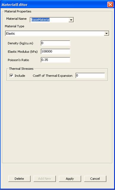
Figure 213. Screen capture. Elastic material properties dialog.
A short explanation of the entry fields is given below.
A.2.3.1. Data Entry Fields
Material Properties Block: These fields are used to input the material properties like density, Poisson's ratio, and elastic modulus.
Thermal Stresses Block: These fields describe the coefficient of thermal expansion of the material. If thermal stresses are to be ignored, then the Include box should be cleared.
A.2.4. Viscoelastic Material Properties Dialog
Figure 214 shows a screenshot of the viscoelastic material properties dialog.
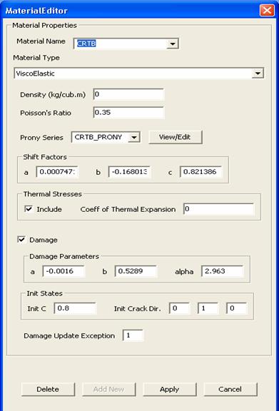
Figure 214. Screen capture. Viscoelastic material properties dialog.
A short explanation of the entry fields is given below.
A.2.4.1. Data Entry Fields
Material Properties Block: These fields are used to input the material properties like density and Poisson's ratio.
Prony Series: This field is used to input the Prony series to be used for characterizing the relaxation modulus of the material. Existing Prony series can be chosen by selecting from the dropdown list. New Prony series can be added by clicking the View/Edit button to invoke the Prony Series dialog. Section A.2.5 describes the configuration of fields on the Prony Series dialog.
Shift Factors Block: These parameters are used along with the Prony coefficients to adjust the material properties for the temperature effects. These parameters are used to find the time-temperature shift factor.
Thermal Stresses Block: These fields describe the coefficient of thermal expansion of the material. If thermal stresses are to be ignored, then the Include box should be cleared.
Damage Parameters Block: These are the parameters for characterizing the damage law as discussed in subsection 2.2.4. If damage effects are to be ignored, then the Damage checkbox should be cleared.
A.2.4.2. Control Actions
View/Edit: This control invokes a Prony series dialog that can be used to add new series or edit an existing series. On successful completion, the identification of the selected/configured series is displayed in the Prony series dropdown list.
Delete: This control is active only when an existing material has been chosen. It can be used to delete the material from the database.
Apply: This control performs validations on the modified/input data, and if no errors are found, it saves the data to the database; however, if the validation fails, an appropriate error message is raised, and the data are not saved to the database. This does not close the dialog on successful completion and can be used to make multiple changes without having to open/close the dialog multiple times.
OK: This is similar to the Apply control in functionality; however, on successful completion, this control saves the data and closes the dialog.
Cancel: This control discards any changes made to the data and closes the dialog.
A.2.5. Prony Coefficients Dialog
Figure 215 shows a screenshot of the Prony Coefficients dialog. This dialog can be used to Add/Edit the Prony series.
Figure 215. Screen capture. Prony Coefficients dialog.
A short explanation of the entry fields is given below.
A.2.5.1. Data Entry Fields
Series Name: This field is a string identification used to uniquely identify the Prony series.
A.2.5.2. Control Actions
Import Data: This control is used to import the Prony coefficients from a text file. Each record in the file is expected to be in the format, "E_i Tai_i", that is, space separated values of Prony coefficients and relaxation times.
Insert Before: This control is used to edit the Prony coefficients table. It adds a new blank row above the current selected row.
Insert After: This control is used to edit the Prony coefficients table. It adds a new blank row below the current selected row.
OK: This control performs validations on the modified data, and if no errors are found, it saves the data and closes the dialog. If validation fails, an appropriate error message is raised.
Cancel: This control discards any changes made to the data and closes the dialog.
A.2.6. Layer Properties Dialog
Figure 216 shows a screenshot of the Layer properties dialog. This dialog is customized depending on the analysis type (2D or 3D). This dialog also supports the configuration of the subgrade as a half-space.
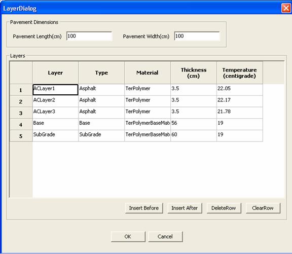
Figure 216. Screen capture. Layer properties dialog.
A short explanation of the entry fields is given below.
A.2.6.1. Data Entry Fields
The fields for this dialog are represented in the form of a table. Each row of the table represents a layer of the pavement. The column headings specify the property being configured. The columns of the table are described as follows:
Pavement Width (cm): This shows the width of the pavement layer. This can be configured only for a 3D analysis.
Pavement Length (cm): This shows length of the pavement section to be simulated. This can be configured only for a 3D analysis.
Layer: This shows a unique string identifying the pavement layer.
Type: This specifies the type of pavement layer. The valid options are AC, Base, SubBase, SubGrade, and InfiniteSubgrade. AC refers to asphalt concrete layer, and InfiniteSubgrade refers to a subgrade that is treated as a half-space. This field is not editable.
Material: This shows the type of material to be associated with the layer. The material can be chosen from the material database that was configured using the Material dialog (section A.2.2).
Thickness: This shows the thickness of the pavement layer. This must be configured for all the layers except if the type of the layer is InfiniteSubgrade. In this case, special elements are used to treat the subgrade as a half-space.
Temperature: This shows the mean temperature in the pavement layer. This is used in adjusting the viscoelastic material properties for the temperature effects.
A.2.6.2. Control Actions
Insert Before: This control adds a pavement layer above the selected pavement layer.
Insert After: This control adds a pavement layer below the selected pavement layer.
DeleteRow: This control deletes the selected pavement layer.
ClearRow: This control clears the selected pavement layer.
OK: This control performs validations on the modified data. If no errors are found, it saves the data and closes the dialog. If validation fails, an appropriate error message is raised.
Cancel: This control discards any changes made to the data and closes the dialog.
A.2.7. Mesh Parameters Dialog
Figure 217 shows a screenshot of the Mesh Parameters dialog. This dialog is used to configure the mesh discretization parameters for the finite element analysis. It is customized depending on ModelType and AnalysisType that were input in the General Information dialog.
The model is divided into the following two zones:
Zone-I: The region corresponding to the actual pavement is called Zone-I. The length and width discretization is common for all the layers, but the thickness discretization can be configured independently for each layer. A uniform discretization is used for each layer.
Zone-II: Zone-II corresponds to the boundary of the pavements and is modeled using infinite elements to simulate the effect of a half-space (semi-infinite medium). A geometric series based discretization is used for each region.
Figure 217. Screen capture. Mesh properties dialog.
A short explanation of the entry fields is given below.
A.2.7.1. Data Entry Fields (Mesh Parameters Block)
Zone-I Length Ratio: This parameter corresponds to the length of the actual pavement. The length is calculated as (Zone-I Length Ratio) multiplied by (Load Length).
Zone-I Length Divisions: This specifies the number of divisions in Zone-I along the length of the pavement.
Zone-I Width Ratio (3D analysis): This parameter corresponds to the width of the actual pavement. The width is calculated as (Zone-I Width Ratio) multiplied by (Load Width).
Zone-I Width Divisions (3D analysis): This corresponds to the number of divisions in Zone-I along the width of the pavement.
Zone-II Mesh Ratio: This specifies the geometric ratio used for creating the geometric series discretization in Zone-II.
Zone-II Init Element Ratio: This parameter corresponds to the initial element size in the geometric series discretization of Zone-II. The initial element size along direction P is calculated as (Zone-II Element Ratio) multiplied by min(element size along perpendicular direction to P).
Zone-II Num Elements: This parameter specifies the number of elements in Zone-II along any direction.
A.2.7.2. Data Entry Fields (Layer Info Block)
The fields Layer, Type, and Thickness are not editable and are taken from the data used to configure the Layer properties.
Divisions: This specifies the number of divisions for the discretization of the pavement layer along the thickness. If the layer is Infinite Subgrade, then this field is also not editable, and the data input from the Zone-II configuration is used.
A.2.7.3. Control Actions
OK: This control performs any validations on the modified data, and if no errors are found, it saves the data and closes the dialog. If validation fails, an appropriate error message is raised.
Cancel: This control discards any changes made to the data and closes the dialog.
A.2.8. Load Properties Dialog
Figure 218 shows a screenshot of the Load properties dialog. This dialog is used to configure the loading conditions for the model. This interface is customized depending on ModelType and AnalysisType fields that were configured using the General Information dialog. In these configurations, the loading area is assumed to be rectangular, and the pressure distributions are assumed to be uniform in the loading area.
Figure 218. Screen capture. Load properties dialog.
A short explanation of the entry fields is given below.
A.2.8.1. Data Entry Fields (Coordinates (in cm) Block)
X: This shows the x coordinate of the load.
Y: This shows the y coordinate of the load.
Z: This shows the z coordinate of the load.
A.2.8.2. Data Entry Fields (Magnitude and Dimensions Block)
Load Magnitude: This parameter corresponds to the load magnitude. The user can choose to specify either the Total Load or Tire Pressure by choosing the appropriate type in the dropdown box. In the screen capture shown in figure 218 the Total Load option is selected.
Load Length: This parameter specifies the length of the loading area. For the pavement problem, this is the length of the tire.
Load Width: This parameter specifies the width of the loading area. For the pavement problem, this is the width of the tire.
A.2.8.3. Data Entry Fields (Moving Load Data Block)
Velocity: This parameter specifies the velocity at which the loading area moves. For the pavement model, this corresponds to the vehicle speed.
A.2.8.4. Control Actions
OK: This control performs validations on the modified data, and if no errors are found, it saves the data and closes the dialog. If validation fails, an appropriate error message is raised.
Cancel: This control discards any changes made to the data and closes the dialog.
A.2.9. Analysis Parameters Dialog
Figure 219 shows a screenshot of the Analysis Parameters dialog, which is used to configure the parameters for the solution algorithm used in the finite element analysis.
Figure 219. Screen capture. Analysis Parameters dialog.
A short explanation of the entry fields is given below.
A.2.9.1. Data Entry Fields
Penalty Number: This parameter corresponds to the Penalty Number used to model stiffness of the rigid members in finite element analysis.
Approximation Scheme Block: The parameters in this block correspond to the parameters used in the Newmark Method approximation scheme.
Iteration Scheme Block: The parameters in this block correspond to the standard parameters for an iterative solution scheme. The analysis engine currently supports only the Newton Iterations.
Prony Configuration Block: Maximum Relaxation Time: This specifies an upper bound on the Prony coefficients configured for the AC Layers.
Prony Configuration Block: Minimum Relaxation Time Factor: This specifies a lower bound on the Prony coefficients configured for the AC Layers. The lower bound is calculated as Min Relaxation Time = (time step size)/(Minimum Relaxation Time Factor).
Simulation Info Block: Simulation Period: This specifies the total simulation time for the analysis.
Simulation Info Block: Num Time Steps: This specifies the number of timesteps that will be used in the simulation and hence fixes the timestep size.
A.2.9.2. Control Actions
OK: This control performs validations on the modified data, and if no errors are found, it saves the data and closes the dialog. If validation fails, an appropriate error message is raised.
Cancel: This control discards any changes made to the data and closes the dialog.
A.2.10. Summary Dialog
Figure 220 shows a screenshot of the Summary dialog, which is used to view a user readable report of the input data.
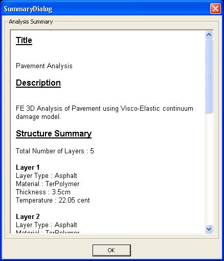
Figure 220. Screen capture. Summary dialog.
A short explanation of the entry fields is given below.
A.2.10.1. Control Actions
OK: This control closes the dialog.
A.2.11. Generating an Input File
The user can generate an input file for FEP++ by choosing the Generate Input File item in the Control Panel. The user is prompted to specify a location for saving the generated file, and the file is created at that location. This can be used to configure multiple analyses and to store the generated input files that can then be run in a batch process.
A.2.12. Running Analysis
Figure 221 shows a screenshot of the view when an analysis is being run. The finite element analysis can be started by clicking the Run Analysis item in the Control Panel. When a user starts a new analysis, it is launched in a separate command window that displays the output from FEP++. Once the analysis is completed, the window is closed, and the results are gathered and stored at the location of the current "db" file.
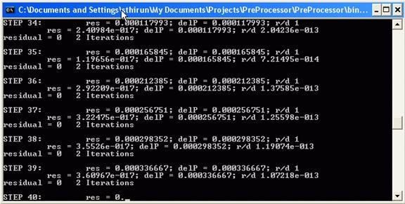
Figure 221. Screen capture. FEP++ analysis in progress.
|


