U.S. Department of Transportation
Federal Highway Administration
1200 New Jersey Avenue, SE
Washington, DC 20590
202-366-4000
Federal Highway Administration Research and Technology
Coordinating, Developing, and Delivering Highway Transportation Innovations
 |
| This report is an archived publication and may contain dated technical, contact, and link information |
|
Publication Number: FHWA-HRT-06-109 Date: September 2006 |
Ricardo Oliveira de Souza
University of Brasilia,
Brasilia, Distrito Federal Brazil
Silvrano Dantas Neto
University of Brasilia,
Brasilia, Distrito Federal Brazil
Faculty Advisor
Márcio Muniz de Farias
University of Brasilia, Brasilia,
Distrito Federal Brazil
This paper presents an analysis between the International Roughness Index (IRI) and the standard deviation of longitudinal roughness (s), as well as a neural network study developed to predict the critical level of roughness. Measured longitudinal profiles available in the Long-Term Pavement Performance (LTPP) program database were used. A total of 207 pavement sections in 42 States of the United States were used to do this analysis. Using a suitable software, the International Roughness Index (IRI) and the standard deviation of longitudinal roughness (s) values were computed for every longitudinal pavement profile measured. Afterwards, these values were used in regression analysis and a high correlation was found between them (R2=0.93). Neural network analysis correlated the IRI-computed values with the type of subgrade soil, pavement structure (layer thickness), climate, and traffic data of 157 pavement sections. The neural network could forecast the IRI with an extremely high correlation factor (R2=0.99). Besides, the neural network provided a sensitivity analysis indicating the relative contribution of factors related to the structural number (49 percent), climate (31 percent), and traffic (20 percent). Multivariate linear and nonlinear statistic regressions were also performed to predict IRI, but no correlation was found.
Longitudinal surface roughness is defined as the deviations over the pavement surface compared to the designed surface grade. These deviations affect the ride quality, the vehicle dynamics, and the effect of dynamic loads over the surface. The difference between the theoretical surface heights and actual surface heights in a longitudinal profile may occur as a result of the construction process, road use, or in some cases a combination of both factors.(1)
The importance of longitudinal surface roughness in users’ comfort perception has been considered since 1960. During the American Association of State Highway Officials (AASHO) Road Test, it was observed that 95 percent of pavement serviceability was related exclusively to the deviations of surface profiles.(2)
The longitudinal roughness is composed of waves whose wavelengths vary as a result of the permanent deformation of the pavement or subgrade under the action of repeated traffic loads. These deviations are presented as waves with intermediate length and amplitude, between 0.5 and 50 meters (m). They are the main source of vehicle dynamic excitation and are responsible for the user’s feeling of discomfort.
Statistics have been developed to represent the longitudinal roughness for measured pavement profiles. A statistic is a numeric value representing the surface deviations for a pavement section. Among them are the slope variance (SV), root-mean square of vertical accelerations (RMSVA), International Roughness Index (IRI), and standard deviation of longitudinal roughness (s).(3)
The longitudinal profiles can be represented by statistics. Some statistics, such as the slope variance (SV) and the standard deviation of longitudinal roughness (s), can be applied directly to the measured longitudinal profile. In other cases, these statistics may apply to imaginary profiles. These imaginary profiles try to represent the relative movement between the rear axle and the vehicle body while the vehicle moves at a certain speed. The longitudinal profiles measured in the field are the input (or dynamic response agent). Through the use of mathematical simulations for the dynamic problem, imaginary profiles can be determined.
Different simulators were developed over the years, such as the quarter car simulator, half car simulator, and whole car simulator. The quarter car simulator, also known as the quarter car system, is the most widely used.(4)
The IRI is a statistic index that summarizes the surface deviations for just one wheel track. This mathematical simulation uses the quarter car system to generate an imaginary profile. As shown in figure 1, the quarter car system is composed of two parts: a sprung mass representing the vehicle body (where the user is seated) and an unsprung mass representing the set of wheel/tire and half axle/suspension. The sprung mass is connected to the unsprung mass by the suspension, which is simulated by a damper and a spring. The sprung mass is in contact with the real pavement surface by another spring.
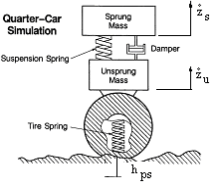
Figure 1. Quarter car simulation.(5)
During the simulation, the quarter car system runs over the longitudinal profile, measured in the field at a constant speed of 80 kilometers per hour (km/h). The roughness over this surface induces dynamic excitation to the quarter car system, generating different vertical speeds (![]() and
and ![]() ) or accelerations (
) or accelerations (![]() and
and ![]() ) in the sprung and unsprung masses. As a result, a relative movement is produced between the chassis and the axle of the imaginary vehicle. The IRI value for a given section length (e.g., 100 m) is computed according to equation 1.
) in the sprung and unsprung masses. As a result, a relative movement is produced between the chassis and the axle of the imaginary vehicle. The IRI value for a given section length (e.g., 100 m) is computed according to equation 1.
![]() (1)
(1)
Where:
IRI = International Roughness Index (in mm/m or m/km).
L = length of the section (m).
x = longitudinal distance (m).
V = speed of the quarter-car model (m/s).
x/V = time the model takes to run a certain distance x.
dt = time increment.![]() = vertical speed of the sprung mass.
= vertical speed of the sprung mass.![]() = vertical speed of the unsprung mass.
= vertical speed of the unsprung mass.
The IRI represents the rectified average slope, or the absolute sum of the relative vertical displacement experienced by the user when driving a fictitious model car over a section (L) of the road at a constant speed of 80 km/h.
A perfectly smooth road results in an IRI value of 0, roads with moderate roughness give IRI values of around 6 meters per kilometer (m/km), and in extreme cases a very bumpy unpaved road can result in IRI values up to 20 m/km.(6) Maintenance intervention threshold varies according to the country, road type, etc. For instance, limit values of 2.7 m/km in the United States, 3.5 m/km in Brazil, 4.0 m/km in Chile, Uruguay, and Spain, and 6.0 m/km in Honduras have been reported.(7) Figure 2 illustrates these threshold differences.
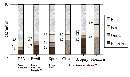
Figure 2. IRI thresholds adopted in different countries.
In Japan, the standard deviation of longitudinal roughness (s) is used to summarize surface deviations. Initially, as illustrates figure 3, the relative difference height “di” (roughness) is measured every 1.5 m, considering an imaginary reference line.(12)
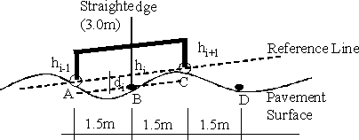
Figure 3. Roughness measurement.(12)
The surface roughness can be measured using a 3-m-long straightedge profilometer (figure 4). Nowadays, laser profilometers are the most used devices. The laser readings are coincident with the desired intervals.
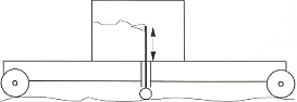
Figure 4. Three-meter-long straightedge profilometer.(13)
During the measurement, hundreds of elevations are registered, thus the heights “di” can be computed according to equation 2.
![]() (2)
(2)
Where:
di = Registered profile heights.
hi, hi-1, hi+1 = Surface elevations.
According to figure 3a, after measuring the height “di” at point B, the beam is displaced to point D, where the heights hi, hi-1, hi+1 are measured at points B, C, and D, respectively. The reference line becomes the line linking points B, C, and D. Using the equation 2 once more, the height “di” at point C can be calculated. When a pavement section is measured continuously, a profile with positive and negative elevations is obtained. These elevations are the relative difference height “di” considering the reference line every 1.5 m.(12)
The longitudinal roughness (s) is computed through the standard deviation of “di” values, as shown in equation 3.
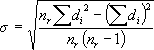 (3)
(3)
Where:
s = Standard deviation of longitudinal roughness (mm).
di = Registered profile heights.
nr = Number of registered data.
The Japan Road Association recommends pavement sections 100 m long to calculate s, whereas the Japan Highway Public Corporation suggests pavement sections 150 m long.(14)
According to Anderson, the neural network concept started with the work of McCulloch and Pitts in 1943.(15) They developed computational elements based on the physiological properties of biological neurons. Later, Widrow-Hoff developed a linear model called ADALINE (ADAptive LINear Element), which was then generalized for multiple layers and called MADALINE (Multiple ADALINE).(16) The next important development came in 1950 with the work of Rosenblatt, who proposed neural networks known as perceptrons. In this model, the network can learn when fed with examples and the responses can assume continuous values, whereas the original neurons of McCulloch-Pitts operated with only binary numbers.(17)
Artificial neural networks (NN) can be understood as a computational technique that helps to develop nonparametric mathematical models. Different from usual statistics techniques, the models do not explicitly exhibit a set of fitting coefficients or parameters (although they are somehow embedded in the model).
The term “neural network” is a little presumptuous and derives from the fact that earlier models were inspired in the neuronal structure of intelligent organisms. However, the technique is rather simple and easy to use. From a mathematical point of view, a neural network is a simple set of points, called nodes or neurons, arranged in a few consecutive layers. There is necessarily an input layer, one or more intermediate layers, and an output layer. The number of input and output neurons depends on the available data and type of problem, whereas the number of intermediate layers and nodes (the NN architecture) is generally a matter of empirical investigation for each case under study. However, there are recent developments in adaptive NN in which the network architecture is iteratively modified during the learning stage.
The neurons of a given layer are generally linked to all neurons of the next layer, although some connections (called synapses) may be disabled and layers may be bypassed. Information is generally processed from the input layer to the output layer in the feed-forward process. A node or neuron (i) of a given layer (t+1) performs very simple mathematical operations. It multiplies each entry Sj(t) from a neuron (j) of the previous (t) layer by some coefficient (wij) and computes the sum (S) of all entries thus modified.
![]() (4)
(4)
The coefficients (wij) are known as synaptic weights and store the main model characteristics during the learning process.
Later, the previous sum (S) is compared to limit value (Øi), known as threshold, for each layer.
![]() (5)
(5)
The value x above will be the argument of function, f(x), known as activation function. The output of this function will be the entry of the neuron for the next layer.
![]() (6)
(6)
Different activation functions may be tried during the development of a model. The most common are the step function and the sigmoid function.
The development of an NN model involves two stages: learning and validation. For that purpose, a sufficiently large number of experimental data must be available. The data with known input and output values are divided into two sets. The first and larger set is used to train the NN and the validation set is used to test the generalization capacity of the trained NN.
The learning stage consists of finding the appropriate synaptic weights (wij) to reproduce the desired output values. The weights are initialized randomly and the computed output values are compared to the desired output values. A root-mean square (RMS) error between computed and desired output values is calculated. Neural networks generally use a learning algorithm known as backpropagation of error. In the backpropagation method, the weights are recalculated from the output layer to the input layer to minimize the RMS error. The process is repeated during several iterations, until a specified error is achieved. This algorithm, also known as the generalized delta rule, is a modification of Widrow-Hoff´s ADALINE, but considers nonlinear activation functions and the entries may assume continuous values. It was developed by Rummerlhart, Hinton, and Williams, and is extremely efficient in minimizing the quadratic error, RMS.(18) Other algorithms are also available.
Once an NN is trained, the validation data set, which was not used in the learning stage, is used to test the forecasting capacity of the model developed. An NN has the property of generalization.
Neural networks are easy to implement, robust even when treating data with some noise, and very efficient, especially when dealing with problems for which a specific knowledge of the underlying mechanisms is not totally available and when analytical formulations are too complicated to be obtained. The use of NN depends on the ability to adapt it to the desired problem by means of appropriate changes in its synaptic weights to enhance its efficiency.
Several commercial and academic programs are available to help develop neural network models. Basically, the user prepares the appropriate input and output files, decides the appropriate NN architecture, and defines a few other analysis parameters. For the analyses in this paper, the authors used a multilayered neural network program called Qnet. The program uses a backpropagation algorithm.
The profile database of the Long-Term Pavement Performance (LTPP) program was used in this study. This program was established in 1984 by the U.S. government as part of the Strategic Highway Research Program (SHRP). The LTPP program consists of two study groups: General Pavement Studies (GPS) and Specific Pavement Studies (SPS). The main objective of GPS is to study the performance of existing pavements constructed by different State departments of transportation in the United States. The selected roads reflect typical materials and structures used in the current practice design in the United States and Canada.(19) The GPS program is divided into 10 subgroups according to the type of pavement structure. Subgroup GPS–1 studies pavements made of asphalt concrete surface course over granular bases. Its database was used for this paper.
The GPS program divided the United States into four main regions and studied sections 152 m long in all States. The LTPP database includes inventory data, climatic data, materials data, maintenance data, rehabilitation data, traffic data, and pavement monitoring data.
In 1992, responsibility for the LTPP program was transferred to the Federal Highway Administration (FHWA), which started to analyze the collected data in 1994. As a result, the first major report was published in 1997. Since then the database has been updated and is available in a CD-ROM software called DataPave, as well as online on the FHWA Web site.
Souza studied the DataPave database, extracting information provided by GPS–1 on about 207 pavement sections in 42 States in the United States.(7) Pavement profiles, obtained with laser profilometers between 1989 and 1996, were retrieved and roughness indices (e.g., IRI and s) were computed using a modified version of the University of Michigan Transportation Research Institute’s (UMTRI) RoadRuf computer program. Each section was surveyed at least once a year and in each instance the measurements were repeated five times. Souza analyzed 6,329 of these profiles and computed thousands of roughness indices, which were later statistically related.(7)
The neural network analysis was done by selecting 57 pavement sections from the 207 sections studied by Souza.(7) These sections contained all of the relevant information, such as layer thickness, climate, and traffic data. Table 1 shows a summary of the minimum, maximum, average, and standard deviation values for the thickness of surface layer course, thickness of binder layer, thickness of base layer, thickness of subbase layer, freezing index, average annual precipitation, number of days with temperature above 32 °C, age of the pavement, average daily volume of heavy vehicles, and computed IRI values. On average, the pavements showed a total asphalt layer course of 15.2 centimeters (cm) and a total granular layer of 32.2 cm. The average climatic conditions show rainfall precipitation of 877 millimeters (mm) per year, with a freezing index of 235 days and 49 days with temperature above 32 °C. The roads were about 18.3 years old and submitted to an average daily volume of 675 heavy vehicles. As to the subgrade conditions, 2 percent of the pavement structures were laid over rock ground, 44 percent on sandy soils, 24 percent on clay soils, 20 percent on gravel, and 10 percent on silt soils.
| Surface Course (cm) | Binder (cm) | Base (cm) | Subbase (cm) | Freeze (F-days) | Rain (mm) | T>32 °C (days) | Age (years) | Traffic Volume | IRI (m/km) | |
|---|---|---|---|---|---|---|---|---|---|---|
| Minimum | 1.0 | 0.0 | 0.0 | 0.0 | 0.0 | 123.0 | 0.0 | 7.0 | 4.0 | 0.62 |
| Maximum | 23.6 | 36.8 | 65.5 | 108.2 | 1530.0 | 2020.0 | 177.0 | 40.0 | 5498.0 | 3.20 |
| Average | 5.6 | 9.6 | 21.5 | 10.7 | 235.4 | 877.0 | 48.8 | 18.3 | 675.0 | 1.45 |
| Deviation | 4.3 | 9.4 | 12.4 | 18.3 | 323.8 | 415.0 | 44.4 | 6.1 | 827.2 | 0.55 |
The analysis of pavement sections was done using a modified version of the UMTRI RoadRuf software. RoadRuf includes several tools developed to interpret the data obtained through longitudinal roughness field measurements. Among these tools are the International Roughness Index (IRI), ride number (RN), and standard filters.(13) Two subroutines were added to the original algorithm to compute the standard deviation of longitudinal roughness (s) and the slope variance (SV).(7)
As illustrated in figure 5, when the computed values of IRI and s were statistically related, a high correlation was observed between them (R2=0.93). The regression model developed (equation 7) can explain 93 percent of the s variation values.
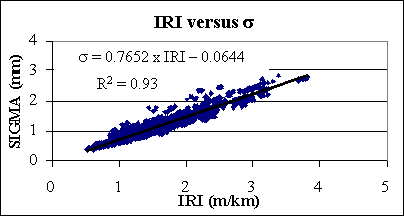
Figure 5. Regression analysis between the IRI and s.
This correlation is impressive since the IRI is computed using a dynamic simulation, whereas s interprets just the geometric characteristics of the pavement surface. This fact refutes the increasing criticisms against the use of indices based exclusively on geometric characteristics.
![]() (7)
(7)
Where:
s = standard deviation of longitudinal roughness (mm).
IRI = International Roughness Index (m/km).
In Japan, the threshold values for the standard deviation of longitudinal roughness (s) varies according to the highway agencies in charge of pavement maintenance. Table 2 illustrates these threshold values and their respective values converted to IRI. The IRI values were computed using the model shown by equation 7.
To analyze the surface condition, IRI and s values were computed for every pavement section to determine the unacceptability of each pavement stretch.
| Pavement Condition | ||
|---|---|---|
| Highway Agency | Recently built pavements (just after construction) |
Pavements in operation (maintenance, conservation) |
| Japan Highway Public Corporation |
1.3 mm (IRI=1.8 m/km) | 2.4 mm (IRI=3.2 m/km) |
| Prefectures (Provinces) | 3.5 mm (IRI=4.7 m/km) | 4.7 mm (IRI=6.2 m/km) |
From: Takashi(20)
According to figure 1, the IRI critical value used by the American Association of State Highway and Transportation Officials (AASHTO) is 2.7 millimeters per kilometer (mm/km), whereas the critical value s adopted by Japan Highway Public Corporation is 2.4 mm (table 2). The IRI and s values computed by the software to each pavement section were compared with admissible values of IRI and s. It was found that of the 207 pavement sections, just 6 presented s values greater than the s critical value. Considering the IRI, it was observed that 8 pavement sections presented index values greater than the critical IRI. Table 3 illustrates the pavement sections whose statistics computed values were greater than the admissible values.
A preliminary comparison between these rejected sections could suggest that the IRI statistic is the most severe because it rejected more pavement sections when compared to the s statistic. However, the higher number of rejected sections may not reflect just the index influence itself, but a difference of strictness between the threshold values considered admissible in the United States (IRI<2.7 m/km) and Japan (s<2.4 mm).
| State | Section | s³2.4 mm | IRI=2.7 m/km | s=2.0 mm |
|---|---|---|---|---|
| Alaska | 1004 | 2.45 | 2.51 | 2.51 |
| Arizona | 1036 | 2.01 | 2.01 | |
| 1037 | 2.27 | 2.27 | ||
| Colorado | 1029 | 2.50 | 2.47 | |
| Illinois | 1003 | 2.40 | 3.16 | 3.16 |
| Kansas | 1005 | 2.40 | 3.00 | 3.00 |
| Kentucky | 1014 | 2.23 | 2.23 | |
| Minnesota | 1016 | 2.26 | 2.26 | |
| 1018 | 2.08 | 2.08 | ||
| 1023 | 2.28 | 2.28 | ||
| 1028 | 2.44 | 2.44 | ||
| 1029 | 2.02 | 2.02 | ||
| 1085 | 2.40 | 3.18 | 3.18 | |
| Nevada | 1021 | 2.00 | 2.00 | |
| New Jersey | 1033 | 2.40 | 3.20 | 3.20 |
| New York | 1643 | 2.07 | 2.07 | |
| Pennsylvania | 1597 | 2.70 | 2.65 | |
| Texas | 1048 | 1.99 | 2.00 | |
| 1049 | 2.70 | 2.67 | ||
| 1056 | 2.01 | 2.01 | ||
| 1065 | 2.16 | 2.16 | ||
| 1096 | 2.33 | 2.33 | ||
| 1111 | 2.14 | 2.14 | ||
| 1178 | 2.43 | 3.12 | 3.12 | |
| 1181 | 2.39 | 2.39 | ||
| 1183 | 2.44 | 2.44 | ||
| Utah | 1004 | 2.94 | 2.94 | |
| Vermont | 1004 | 2.13 | 2.13 | |
| Virginia | 1002 | 2.41 | 2.41 | |
| 1423 | 2.07 | 2.07 | ||
| Sum total | 6 | 8 | 30 | |
This kind of comparison is trustworthy only if the roughness statistics are analyzed considering the same admissible values references. Using the regression model developed (equation 7), the s computed values were converted to the IRI index. The admissible IRI (IRI=2.7 m/km) is equivalent to a critical s value of 2 mm. The pavement sections whose s values are greater than 2 mm are also included in table 3.
Of the 207 pavement sections, just 30 sections presented s roughness values higher than 2 mm. Thus, 30 sections would be rejected according to this criterion. These rejected pavement sections now can be compared to the sections rejected by the IRI statistic, since both use the same reference (IRI=2.7 m/km and s (converted to IRI)=2 mm). Since the number of s rejected sections is higher than the IRI rejected sections, the s statistic is more strict or rigorous than the IRI statistic.
Using the regression model presented by equation 7, an analysis of the s acceptance threshold was achieved. It was noted that the admissible (s=2.4 mm) value is equivalent to a critical IRI of 3.2 m/km. This shows that the acceptance threshold values are stricter in the United States.
Prediction of Longitudinal Roughness Using Neural Networks
The previously described IRI data was initially analyzed using the Qnet neural network modeling system with the objective of finding an NN model as function of the available input parameters. A single output layer for IRI value was used. The input layer consisted of 10 data neurons as follows:
The subgrade soil was divided in 14 types according to the Unified Soil Classification System (SUCS), plus rock foundation. The following codes were attributed to input 5 (SG): Rock=0, SC=1, SW–SM=2, SP=3, SP–SM=4, SM=5, CL=6, CL–CM=7, GC=8, GP=9, GP–GM=10, GC–GM=11, GM=12, GW=13, and MH=14.
A few neural network architectures were tried to find the best configuration for the intermediate layers. The best results were obtained for the configuration illustrated in figure 6, with three intermediate layers of eight, five, and three neurons, respectively. All neurons of a given layer are connected to all neurons of the subsequent layer. A sigmoid activation function was used.
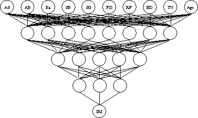
Figure 6. Adopted neural network model.
A training data set comprising 140 random sections out of 157 available (89 percent) was initially chosen for the learning stage. The NN of figure 6 produced excellent results, as illustrated in figure 7, which shows the training targets (measured IRI values) in the abscissa and the network outputs (computed IRI values) in the ordinate. The correlation coefficient for the learning stage was very high with R2=0.992. The root-mean square error was RMS=0.017.
After the training stage, the remaining 17 sections were used to validate the model. Predictions were also good, despite a higher dispersion than in the learning stage (figure 8). The correlation coefficient for the validation stage was R2=0.80 with a standard deviation of IRI values equal to 0.28. The lower correlation of the validation stage may be attributed to the relatively small number of sections available or to an overfitting during the learning stage.
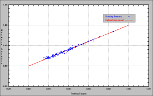
Figure 7. Learning stage.
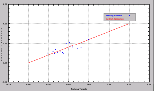
Figure 8. Validation stage.
An important feature of the Qnet program is that it allows quantification of the relative contribution of each input neuron to the computed output value. Hence, it is possible to investigate the most relevant factors affecting roughness in a flexible pavement. Individual contributions of each input are shown in table 4. In the same table, the contributions were grouped for the pavement structure (38.1 percent), climatic factors (31.2 percent), and traffic conditions (20.4 percent), besides subgrade type (10.3 percent).
| Input | 1 | 2 | 3 | 4 | 5 | 6 | 7 | 8 | 9 | 10 |
|---|---|---|---|---|---|---|---|---|---|---|
| SC | AB | Ba | SB | SG | FD | RF | HD | TV | Age | |
| Contribution (%) | 10.44 | 9.46 | 10.81 | 7.39 | 10.3 | 11.39 | 7.94 | 11.86 | 10.22 | 10.18 |
| Structure | Subgrade | Climate | Traffic | |||||||
| Contribution (%) | 38.1 | 10.3 | 31.2 | 20.4 | ||||||
The same IRI data values were used to try to establish statistical models using SYSTAT® software. The user defines a priori the type of model to be tried. In this paper, multivariate linear and nonlinear (exponential) models were tested. The model constants and correlation coefficients are shown in table 5. A plot of computed-versus-target IRI values for both models is shown in figure 9. Dispersion is complete and no correlation at all could be found with R2=0.15 and R2=0.21 at best for the linear and nonlinear models, respectively.
| Linear |
Nonlinear |
|||
|---|---|---|---|---|
| Input | xi | Ai | Ai | Bi |
| SC | 1 | -0.229 | 1.138 | -0.237 |
| AB | 2 | 0.033 | 0.735 | -0.119 |
| Ba | 3 | 0.006 | 1.287 | -27.130 |
| SB | 4 | -0.015 | 0.414 | -0.117 |
| SG | 5 | -0.151 | 0.376 | -0.277 |
| FD | 6 | -0.004 | 1.598 | -0.228 |
| RF | 7 | -0.005 | 22.355 | -0.479 |
| HD | 8 | -0.037 | 0.682 | -0.156 |
| TV | 9 | -0.001 | 2.229 | -0.058 |
| Age | 10 | 0.019 | 11.390 | -960.900 |
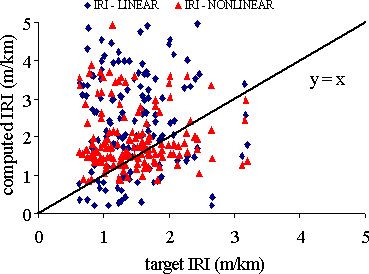
Figure 9. Computed-versus-target IRI values for both statistical models.
The International Roughness Index (IRI) and the standard deviation of longitudinal roughness (s) were correlated for 6,329 pavement longitudinal profiles measured on 207 pavement sections of the LTPP program. A high correlation was found between the IRI and s statistics (R2=0.93).
When the IRI and s statistics were compared under different references, it was observed that the IRI rejected a higher number of pavement sections. However, when the IRI and s statistics were equated using the regression model developed in this study, it was found that the s statistic rejected more pavement sections than the IRI. Therefore, the s statistic is stricter than the IRI statistic.
Using the regression model developed in this study, it was also found that the roughness acceptance threshold values are stricter in the United States than in Japan.
Neural network and multivariate statistics regression were used to try modeling the computed IRI values. Out of 207 pavement sections, 157 sections were selected to achieve this study. A complete set of subgrade, pavement structure, climate, and traffic data and IRI computed values for each pavement measured profile were available.
An extremely accurate model using Qnet neural network software was developed. This NN model gave a coefficient of correlation of 0.992 during the learning stage. Despite a lower correlation during the validation stage, it is believed that this feature can be improved as more data become available. On the other hand, it was not possible to model the data using multivariate linear and nonlinear (exponential) statistics models.
The studied database (GPS–1) comprised concrete asphalt pavements with granular base and subbase over most U.S. States, covering a wide range of subgrade soils and climatic and traffic conditions. The NN model allowed quantification of the relative contributions of these factors on IRI values and credited most of the pavement roughness (around 49 percent) to structural factors (subgrade soil and pavement layer thickness), followed by climatic factors (31 percent) and traffic conditions (20 percent). The most important structural factor was the overall thickness of the asphalt layers (including binder), responsible for almost 20 percent of the roughness index. However, these numbers should not be extrapolated to other countries with different engineering practices and less rigorous traffic weight control.
The neural network proved to be an extremely powerful tool to predict pavement roughness. Similar NN models may be developed for other databases of LTPP’s GPS program to include other types of pavement structures.
The authors acknowledge the financial support of Brazilian agencies Conselho Nacional de Desenvolvimento Científico e Tecnológico (CNPq) and Coordenação de Aperfeiçoamento de Pessoal de Nível Superior (CAPES).
Río, R.C. (1999). “Tread quality.” Jornadas sobre la calidad en el proyecto y la construcción de carreteras. AEPO Ingenieros Consultores, Barcelona, Spain. (In Spanish). At http://www.aepo.es/aepo-old/ausc/publ/calidad.pdf.
Haas, R., Hudson, W.R., and Zaniewski, J. (1994). Modern Pavement Management. Melbourne, FL: Krieger Publishing Co.
Farias, M.M., and Souza, R.O. (2002). “Longitudinal roughness and its influence on pavement functional evaluation.” Proceedings VII National Meeting for Highways Conservation. CD-ROM. Vitória, Brazil. (In Portuguese).
Melis, M., and Río, R.C. (1992). “IRI computation through highway longitudinal profile. The IRI once more. The IRI equation for a sinusoidal profile.” Cuaderno AEPO No 1. AEPO Ingenieros Consultores, Madrid, Spain. (In Spanish).
Shahin, M.Y. (1994). Pavement Management for Airports, Roads and Parking Lots. Norwell, MA: Kluwer Academic Publishers.
Paterson, W.D.O. (1987). Road Deterioration and Maintenance Effects: Models for Planning and Management. Highway Design and Maintenance Standard Series. Baltimore, MD: The John Hopkins University Press.
Souza, R.O. (2002). “Influence of Longitudinal Roughness on the Evaluation of Pavement.” M.S. Dissertation. Pubication 625.8(043) S729i. University of Brasilia, Brasilia, Brazil. (In Portuguese).
U.S. Department of Transportation. (1999). Status of the Nation's Highways, Bridges, and Transit: Conditions and Performance. Report to the U.S. Congress. Washington, DC. At https://www.fhwa.dot.gov/policy/1999cpr/report.htm.
Pinto, S., and Preussler, E. (2001). “Pavimentação Rodoviária. Conceitos fundamentais sobre pavimentos flexíveis.” Copiarte, Copiadora e Artes Gráficas Ltda. Rio de Janeiro, Brazil. (In Portuguese).
Río, R.C. (1997). “Introduction to pavements sounding.” Cuaderno AEPO No. 4. AEPO Ingenieros Consultores, Madrid, Spain. (In Spanish). At http://www.aepo.es/aepo-old/ausc/publ/auscultacion.pdf.
Patiño, M.C.A., and Anguas, P.G. (1998). “International Roughness Index, application to the Mexican highway network.” Publicación Técnica No. 108. Instituto Mexicano del Transporte, Sanfandila, Querétaro, Mexico. (In Spanish).
Suzuki, K. (2001). Personal Communication. Japan Highway Public Corporation, Tokyo, Japan.
Sayers, M., and Karamihas, S.M. (1996). The Little Book of Profiling: Basic Information about Measuring and Interpreting Road Profiles. University of Michigan Transportation Research Institute, Ann Arbor, MI.
Japan Road Association (1989). Manual for asphalt pavement. Second Edition. Tokyo, Japan.
Anderson, A.J. (1995). An Introduction to Neural Networks. Cambridge, MA: MIT Press.
Kovács, L.Z. (1997). Artificial Neural Networks: Fundamentals and Applications (20 ed.). Editora Collegium Cognitio e Edição Acadêmica. (In Portuguese).
Fausett, L. (1994). Fundamentals of Neural Networks: Architectures, Algorithms, and Applications. Englewood, NJ: Prentice-Hall.
Hertz, J.A., Krogh, A., and Palmer, R. G. (1991). Introduction to the Theory of Neural Computation. New York: Addison-Wesley Publishing Co.
Federal Highway Administration. (2001). DataPaveVersion 3.0. Washington, DC. At http://www.datapave.com/.
Takahashi, S. (2001). Personal Communication. Japan Highway Public Corporation, Tokyo, Japan.

