U.S. Department of Transportation
Federal Highway Administration
1200 New Jersey Avenue, SE
Washington, DC 20590
202-366-4000
Federal Highway Administration Research and Technology
Coordinating, Developing, and Delivering Highway Transportation Innovations
 |
| This report is an archived publication and may contain dated technical, contact, and link information |
|
Publication Number: FHWA-RD-07-052 Date: September 2007 |
This appendix contains the algorithms used to determine the resilient modulus, creep compliance and indirect tensile strength for specimens tested using the P07 testing protocol. The algorithms presented herein are based upon the data format, data sampling rates and file structures used for LTPP P07 testing purposes. If formats, sampling rates or file structures used are different than outlined herein, the algorithms should be modified appropriately.
These algorithms are based upon the methods developed by Dr. Reynaldo Roque et al. and documented in the report referenced in Section 4.4 of this protocol. Dr. Roque and his colleagues developed two programs: MRFHWA to reduce and analyze resilient modulus data, and ITLTFHWA to reduce and analyze creep compliance and indirect tensile strength data. The user's guide for the software is available as a separate document. The data analysis methods used in MRFHWA and ITLTFHWA are documented in this appendix.
This appendix is divided into four sections as follows:
B1. Introduction
B2. Resilient Modulus Data Analysis Algorithm
B3. Creep Compliance Data Analysis Algorithm
B4. Indirect Tensile Strength Analysis Algorithm
An outline of the resilient modulus data analysis algorithm that is used in the "MRFHWA" software, and described in the report by Roque et al. is presented in section B2.2. The algorithm is described graphically in section B2.3.
B2.1 Subscript Convention
For the purpose of clarity, a subscript convention has been developed. The subscript 'i' represents the specimen number (i = 1, 2, or 3), the subscript 'j' represents the cycle number (j = 1, 2, or 3), and the subscript 'k' represents the specimen face (k = 1 or 2). Thus a variable may have up to three subscripts of the following form: Xi,j,k.
B2.2 Analysis
A separate analysis must be performed for each of the three temperatures.
B2.2.1 Select Cycles
For each of the three specimens, determine which three cycles of the five recorded in the data file shall be used for analysis. Find the maximum load (Pmax) of the first recorded cycle in the data file. If the maximum occurs at or after 150 points from the start of the file, then the first three cycles recorded in the data file shall be used for subsequent analysis. If the maximum occurs less than 150 points from the start of the file, then the second, third and fourth cycles recorded in the test shall be used. From now on, regardless of which cycles have been selected for analysis, they shall be referred to as cycles 1, 2 and 3, respectively.
B2.2.2 Calculate Contact Load (Pcontacti)
For each of the three specimens calculate the contact load. Only one contact load shall be calculated for each specimen as follows:
(1) Determine the point at which the maximum load (Pmax) occurs for cycle 1.
(2) Select the range of cells from 80 points before Pmax to 30 points before Pmax (50 points total)
(3) Average the load values in the selected range as follows:
Eq. B1: 
where: Pcontacti = the contact load for specimen i, lbs.
Py = the load at point y, lbs.
x = the point at which Pmaxi,1 occurs
B2.2.3 Determine Cycle Start and End Points
For each cycle j on each specimen i, determine the start and end points as follows. Determine Pmax for cycle j
(1) Starting at Pmax, and moving to the left, the start of cycle j is defined as the last data point for which the load is greater than Pcontacti + 6 lbs (2.7 kg). This value shall be referred to as spi,j.
(2) Starting at Pmax and moving to the right, the end point for cycle j is defined as the last data point for which the load is less than Pcontacti + 6 lbs (2.7 kg). This value shall be referred to as epi,j.
B2.2.4 Determine the Cyclic Load
For each cycle j on each specimen i, determine the cyclic load (Pcyclici,j) as follows:
Eq. B2: Pcyclici, j = Pmaxi, j Pcontacti
where: Pcyclici,j = the cyclic load for cycle j of specimen i, lbs.
Pmaxi,j = the maximum load for cycle j of specimen i, lbs. Pcontacti = the contact load of specimen i, lbs
B2.2.5 Calculate the maximum deformations:
On each of the two sawn faces of the sample, deformations are measured in the horizontal and vertical axes. Thus for each sample there will be a total of four deformation vs. time traces. From each of these traces, pick off the maximum deformation for each of the three cycles, within the cycle start and end points defined in section B2.2.3. These deformations will be referred to in the following format:
{H,V}maxi,j,k, inches
where {H,V} refers to the axis in which the deformation was measured (horizontal or vertical) and subscripts i, j and k refer to the specimen, cycle and face, as defined in section B2.1.
B2.2.6 Determine minimum deformations:
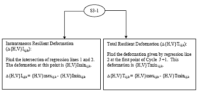
For {H,V}maxi,j,k calculated in section 4.2.5 there will be two corresponding minimum deformations: Total and Instantaneous, as shown in Figure 3 of the main body of this procedure. To calculate these minimum deformations two regression lines must be developed. These minimum deformations shall be referred to in the following format:
{H,V}min{I,T}i,j,k, inches
where {H,V} refers to the axis in which the deformation was measured (horizontal or vertical), {I,T} refers to the type of deformation (instantaneous or total) and subscripts i, j and k refer to the specimen, cycle and face, as defined in section B2.1.
To calculate {H,V}min{I,T}i,j,k, two regression lines must be developed from the deformation vs. time trace.
B2.2.6.1 Regression Line 1
(1) Starting at {H,V}maxi,j,k and moving to the right, select the 5th through 17th data points (13 data points total).
(2) Perform a least squares linear regression on deformation vs. time for the selected data points. The resulting equation shall be as follows:
Eq. B3 ![]()
Where: m1 = the slope of regression line 1, and
b1 = the Y-intercept of regression line 1
B2.2.6.2 Regression Line 2
(1) Starting at the start point of cycle j+1 and moving to the left, select first 300 data points (300 data points total).
(2) Perform a least squares linear regression on deformation versus time for the selected data points. The resulting equation shall be as follows:
Eq. B4 ![]()
Where: m2 = the slope of regression line 2, and
2 = the Y-intercept of regression line 2
B2.2.6.3 Calculate {H,V}minI i,j,k
{H,V}minIi,j,k is the deformation at the intersection of regression lines 1 and 2.
Eq. B5 ![]()
B2.2.6.4 Calculate {H,V}minTi,j,k {H,V}minTi,j,k is the deformation calculated from regression line 1 and the first point of cycle j+1
Eq.B6 ![]()
B2.2.7 Calculate the total and instantaneous recoverable deformations
The total and instantaneous recoverable deformations shall be referred to as D{H,V}Ti,j,k and D{H,V}Ii,j,k respectively.
Eq. B7 ![]()
B2.2.8 Calculate average thickness and diameter
Eq. B8 
Eq. B9 
Where: tavg = the average thickness for all the specimens, inches
ti = the thickness of specimen i, in
davg = the average thickness for all the specimens, inches
di = the diameter of specimen i, in
vB2.2.9 Calculate the average cyclic load
Eq. B10 
Where: Pavgj = the average cyclic load for cycle j, lbs.
Pcyclici,j = the cyclic load for cycle j of specimen i, lbs.
B2.2.10 Calculate the deformation normalization factors
Eq. B11 
Where: Cnormi,j = the deformation correction factor for cycle j of specimen i,
ti = the thickness of specimen i, in.
tavg = the average thickness of the specimens, in.
di = the diameter of specimen i, in.
davg = the average diameter of the specimens, in.
Pcyclici,j = the cyclic load for cycle j of specimen i, lb.
Pavgj = the average cyclic load for cycle j lb.
B2.2.11 Calculate the normalized deformations
Eq. B12 ![]()
Where: D{H,V}{I,T}ni,j,k = the normalized deformation for face k and cycle j of specimen i, in.
Cnormi,j = the deformation correction factor for cycle j of specimen i,
D{H,V}{I,T}i,j,k = the deformation for face k and cycle j of specimen i, in.
B2.2.12 Average deformation data sets
There are 12 deformation data sets. A deformation data set consists of all the recoverable deformations calculated for a given axis {H,V}, measurement point {I,T} and cycle j. Average the deformation data sets by one of the following methods:
B2.2.12.1 Method 1: Normal Analysis
For each deformation data set, remove the highest and lowest deformation and average the remaining four. This average shall be referred to as D{H,V}{I,T}navgj
B2.2.12.2 Method 2: Variation of Normal Analysis
For each deformation data set, remove the tow highest and the two lowest deformations and average the remaining two. This average shall be referred to as D{H,V}{I,T}navgj
B2.2.12.3 Method 3: Individual Analysis
For each deformation data set, remove any deformations and average the remaining deformations. This average shall be referred to as D{H,V}{I,T}navgj
B2.2.13 Calculate Poisson's ratios
Eq. B13 
B2.2.14 Calculate the cycle averaged deformations
Eq. B14 
B2.2.15 Calculate the resilient modulus correction factors
Eq. B15 
B2.2.16 Calculate resilient modulus
Eq. B16 
B2.2.18 Repeat sections B2.2.1 through B2.2.17 for each temperature.
B2.3 Resilient Modulus Data Analysis Algorithm Flowchart
B2.3.1 Main Procedure
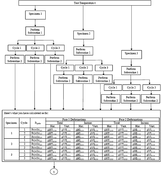
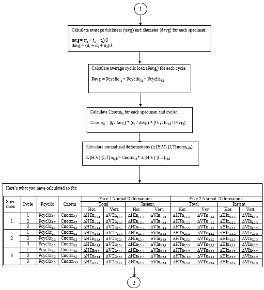
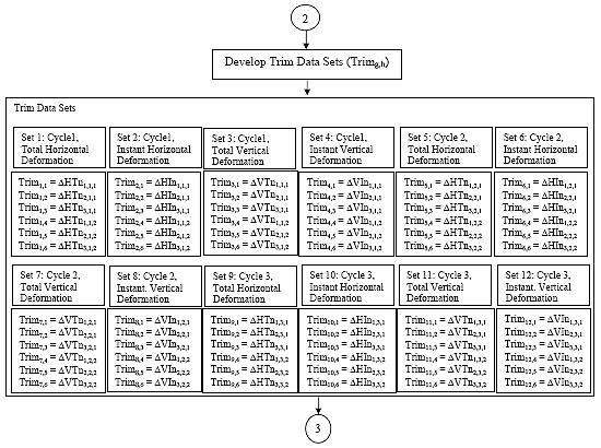
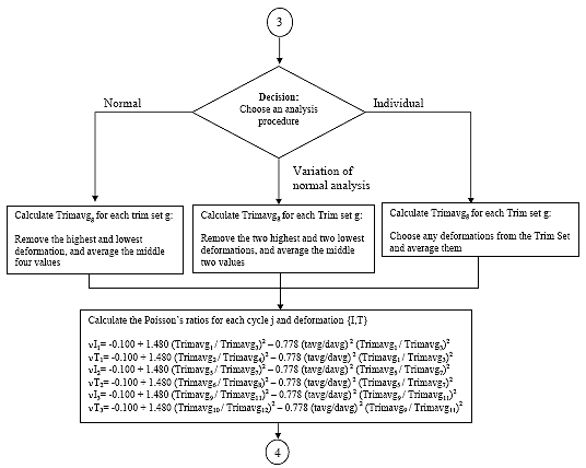
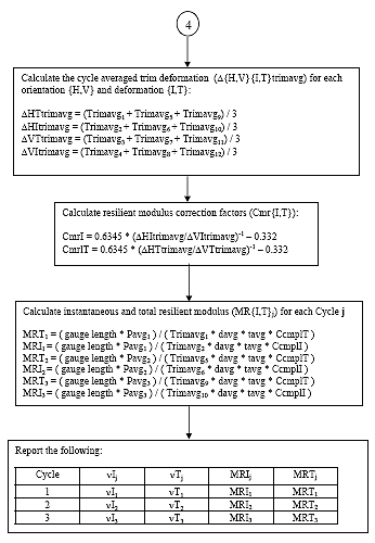
B2.3.2 Subroutine 1
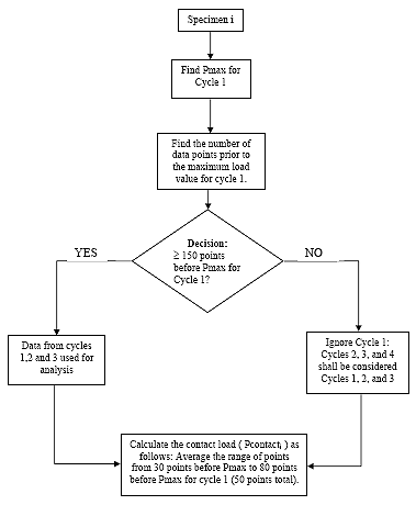
B2.3.3 Subroutine 2
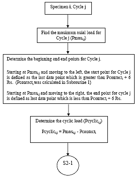
B2.3.4 Subroutine 3
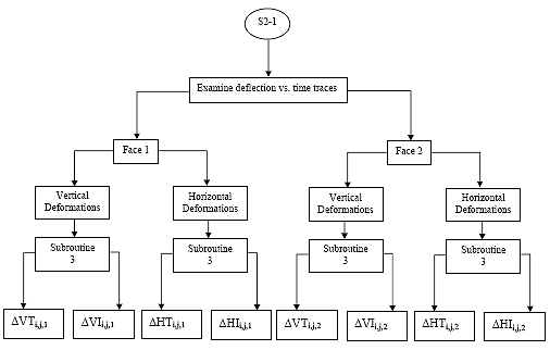
An outline of the creep compliance data analysis algorithm that is used in the "ITLTFHWA" software, and described in the report by Roque et al. is presented in section B3.2. The algorithm is described graphically in section B3.3.
B3.1 Subscript Convention
For the purpose of clarity, a subscript convention has been developed. The subscript 'i' represents the specimen number (i = 1, 2, or 3), the subscript 'j' represents the creep time (j = 1, 2, 5, 10, 20, 50, or 100), and the subscript 'k' represents the specimen face (k = 1 or 2). Thus a variable may have up to three subscripts of the following form: Xi,j,k.
B3.2 Analysis
A separate analysis must be performed for each of the three temperatures at which creep compliance data is collected.
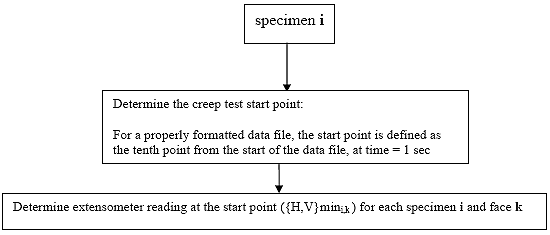
B3.2.1 Determine the creep test start point
The 10th data point in the file is always assumed to be the starting point of the test. It is essential that when the test is performed that exactly 10 data points are collected prior to the initial application of the creep load otherwise this analysis algorithm will produce erroneous results. Since the data sampling rate should be constant at 10 Hz, the creep load should be applied exactly 1 second after the data acquisition is initiated.
B3.2.2 Determine initial extensometer readings
Determine the extensometer reading ({H,V}mini,k) at the starting point of the creep test for each specimen i and face k. The starting point was defined in Section B3.2.1.
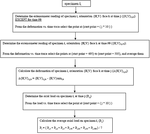
B3.2.3 Determine the extensometer reading for each creep time j
The Table B2 indicates the data point that corresponds to a certain creep time j for each face k of each specimen i.
| Extensometer reading at time j | Data Point |
|---|---|
| {H,V}i,1,k | 20th point in data file |
| {H,V}i,2,k | 30th point in data file |
| {H,V}i,5,k | 60th point in data file |
| {H,V}i,10,k | 110th point in data file |
| {H,V}i,20,k | 210th point in data file |
| {H,V}i,50,k | Average 505th point through 515th point (11 points total) |
| {H,V}i,100,k | 1010th point in data file |
For a 100-second creep test, the deformations at 50 seconds are used to calculate the Poisson's ratio for the experiment. To prevent a spike in the data from influencing the Poisson ratio value, the average of the 505th point through the 515th point (11 points total) is taken as the deformation at 50 seconds.
B3.2.4 Calculate deformations for each creep time j, face k, and orientation {H,V} of each specimen i.
Eq. B20 ![]()
Where: D{H,V}i,j,k = the deformation for creep time j of face k of each specimen i, in.
{H,V}i,j,k = the extensometer reading for creep time i of face k of each specimen i, in.
{H,V}mini,k = the extensometer reading at the start of the creep test for each face k of each specimen i, in.
B3.2.5 Determine the axial load (Pi,j) for each creep time j of each specimen i.
| Axial load at time j | Data Point |
|---|---|
| Pi,1 | 20th point in data file |
| Pi,2 | 30th point in data file |
| Pi,5 | 60th point in data file |
| Pi,10 | 110th point in data file |
| Pi,20 | 210th point in data file |
| Pi,50 | 510th point in data file |
| Pi,100 | 1010th point in data file |
B3.2.6 Determine the average axial load (Pi) on specimen i
Eq. B21 
where: Pi = the average axial load for specimen i, lbs.
Pi,t = the axial load for specimen i at time = t, lbs.
B3.2.7 Calculate the average specimen thickness (tavg), the average specimen diameter (davg), and the average axial load (Pavg).
Eq. B22 
Where: tavg = the average specimen thickness, in.
davg = the average specimen diameter, in.
Pavg = the average axial load, lbs.
ti = the thickness of specimen i, in.
di = the diameter of specimen i, in.
Pi = the axial load for specimen i, lbs.
B3.2.8 Calculate the deformation normalization factor (Cnormi) for each specimen i.
Eq. B23 
Where: Cnormi = the deformation normalization factor for specimen i.
tavg = the average specimen thickness, inches.
davg = the average specimen diameter, inches.
Pavg = the average axial load, lbs.
ti = the thickness of specimen i, inches.
di = the diameter of specimen i, inches.
Pi = the axial load for specimen i, lbs.
B3.2.9 Calculate the normalized deformations (D{H,V}normi,j,k) for time j and face k of each specimen i.
Eq. B24 ![]()
Where: D{H,V}normi,j,k = the normalized deformations for time j and face k of specimen i, inches.
D{H,V}i,j,k = the deformation for creep time j of face k of each specimen i, inches.
Cnormi = the deformation normalization factor for specimen i.
B3.2.10 Average deformation data sets
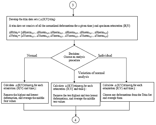
There are 14 "trim" data sets. A deformation data set consists of all the recoverable deformations calculated for a given orientation {H,V}, and time j. Average the deformation data sets by one of the following methods:
B3.2.10.1 Method 1: Normal Analysis
For each trim data set, remove the highest and lowest deformation and average the remaining four. This average shall be referred to as D{H,V}trimavgj for time j.
B3.2.10.2 Method 2: Variation of Normal Analysis
For each trim data set, remove the two highest and the two lowest deformations and average the remaining two. This average shall be referred to as D{H,V}trimavgj for time j.
B3.2.10.3 Method 3: Individual Analysis
For each trim data set, remove any deformations and average the remaining deformations. This average shall be referred to as D{H,V}trimavgj for time j.
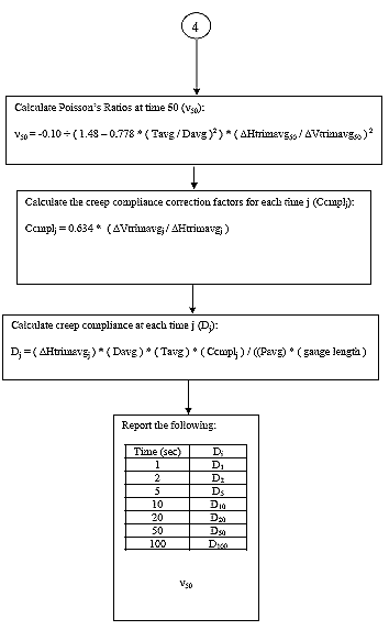
B3.2.11 Calculate the Poisson's Ratio at time = 50.
Eq. B25 
Where: ? = the Poisson's Ratio
DHtrimavg50 = the average horizontal trimmed deformation at time = 50, in.
DVtrimavg50 = the average vertical trimmed deformation at time = 50, in.
tavg = the average specimen thickness, in.
davg = the average specimen diameter, in.
B3.2.12 Calculate the creep compliance correction factor (Ccmply) for each time j.
Eq. B26 
Where: Ccmplj = the creep compliance correction factor at time j.
DHtrimavgj = the average horizontal trimmed deformation at time j, in.
DVtrimavgj = the average vertical trimmed deformation at time j, in.
B3.2.13 Calculate the creep compliance for each time j.
Eq. B27 
Where: Dj = the creep compliance at time j, 1/psi
DHtrimavgj = the average horizontal trimmed deformation at time j, in.
davg = the average specimen diameter, in.
tavg = the average specimen thickness, in.
Ccmplj = the creep compliance correction factor at time j.
Pavg = the average axial load, lbs.
GL = the extensometer gauge length (1 inch [25 mm] for a nominal 4-inch [102-mm] specimen diameter, 1.5 inches [38 mm] for a nominal 6-inch [152-mm] specimen diameter).
B3.3 Creep Compliance Data Analysis Flow Charts
B3.3.1 Main Procedure
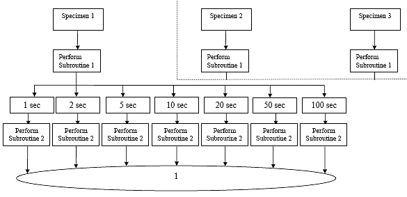
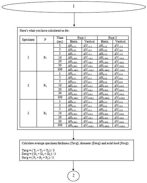
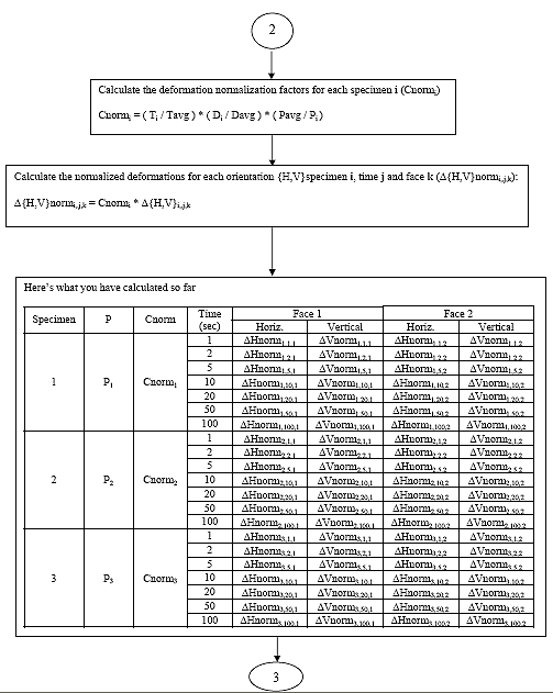
B3.3.2 Subroutine 1
B3.3.3 Subroutine 2
An outline of the indirect tensile strength algorithm that is used in the "ITLTFHWA" software, and described in the report by Roque et al. is presented in section B4.2. The algorithm is described graphically in section B4.3.
B4.1 Subscript Convention
For the purpose of clarity, a subscript convention has been developed. The subscript 'i' represents the specimen number (i = 1, 2 or 3), the subscript 'j' represents the specimen face (j =1 or 2) and the subscript 't' represents the time at which a value was measured. Thus a variable may have up to three subscripts of the following form: Xi,j,t.
B4.2 Analysis
B.4.2.1 Invert Load Values
For each of the three specimens, multiply all load values by -1, so that compression values are positive.
B.4.2.2 Determine Cycle Start Time (tsi):
For specimen i, determine the time at which the load cycle starts. The load cycle start time is defined as the first time t that satisfies the following two requirements:
1) The load must continuously increase over the three data points subsequent to tsi, as shown below:
Eq. B28 ![]()
2) The load must increase by at least 40 lbs (18 kg) over the three data points subsequent to tsi, as shown below:
Eq. B29 ![]()
B4.2.3 Zero the Time Values
For each specimen i, subtract tsi from each time value, so that the load cycle starts at t = 0.
B4.2.4 Zero the Load Values
For each specimen i, subtract the initial load value, Pi,0 from each load value, so that the load at the time the cycle starts is 0.
B4.2.5 Calculate the Deformation Zero Value ({H,V}si,j)
For each specimen i, face j, and orientation {H,V}, the deformation zero value is equal to the average of the 10 deformation values prior to the load cycle start, as shown below:
Eq. B30 
B4.2.6 Zero the Deformation Values
For each specimen i, face j, and orientation {H,V}, subtract {H,V}si,j from the respective deformation value.
B4.2.7 Determine the Failure Load (Pi,tfi)
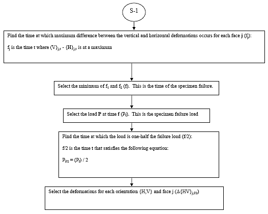
B4.2.7.1 Determine tfi,j
For each specimen i, and face j, determine the time where Vi,j,t - Hi,j,t is at a maximum (tfi,j).
B4.2.7.2 Determine Time of Specimen Failure (tfi)
For each specimen i, the time of specimen failure (tfi) is the minimum of tfi,1 and tfi,2.
B4.2.7.3 Determine the Failure Load (Pi,tfi)
For each specimen i, the failure load is the load P corresponding to time tfi.
B4.2.9 Determine the Deformations at Half the Failure Load (?{H,V}i,j)
B4.2.9.1 Determine the Time of Half Failure Load (thi)
For each specimen i, thi is the time that satisfies the following equation:
Eq. B31 ![]()
B4.2.9.2 Determine Deformations at Time thi
For each specimen i, face j and orientation {H,V}, select the deformations at time thi. This value shall be referred to as ?{H,V}i,j.
B4.2.10 Calculate the Average Specimen Thickness and Diameter
Calculate the average specimen thickness (Tavg) and diameter (Davg) as shown below:
Eq. B32 
Eq. B33 
B4.2.11 Calculate the Deformation Normalization Factors (Cnormi)
For each specimen i, calculate the deformation normalization factors as shown below:
Eq. B34 
B4.2.12 Calculate the Normalized Deformations (?{H,V}normi,j)
Eq. B35 ![]()
B4.2.13 Average deformation data sets
There are 2 "trim" data sets. A deformation data set consists of all the normalized deformations calculated for a given orientation {H,V}. Average the deformation data sets by one of the following methods:
B4.2.13.1 Method 1: Normal Analysis
For each trim data set, remove the highest and lowest deformation and average the remaining four. This average shall be referred to as D{H,V}trimavg.
B4.2.13.2 Method 2: Variation of Normal Analysis
For each trim data set, remove the two highest and the two lowest deformations and average the remaining two. This average shall be referred to as D{H,V}trimavg.
B4.2.13.3 Method 3: Individual Analysis
For each trim data set, remove any deformations and average the remaining deformations. This average shall be referred to as D{H,V}trimavg.
B4.2.14 Calculate Poisson's Ratio (?)
Eq. B36 
B4.2.15 Calculate "Used" Poisson's Ratio (?used)
B4.2.15.1 Case 1: ? > 0.5
If the ? calculated in step B4.2.14 is greater than 0.5, then ? used = 0.5.
B4.2.15.2 Case 2: ? < 0.05
If the ? calculated in step B4.2.14 is less than 0.05, then ? used = 0.05.
B4.2.15.3 Case 3: 0.05 < ? < 0.5
If the ? calculated in step B4.2.14 is between 0.05 and 0.5, then ? used = ?.
B4.2.16 Calculate the Stress Correction Factors
For each specimen i, calculate the stress correction factors as follows:
Eq. B37 
B4.2.17 Calculate the Indirect Tensile Strength
For each specimen i, calculate the indirect tensile strength as follows:
Eq. B38 
B4.2.18 Calculate the Average Indirect Tensile Strength
Eq. B39 
B4.3 Indirect Tensile Strength Analysis Flowcharts
B4.3.1 Main Procedure
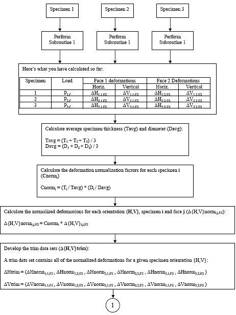
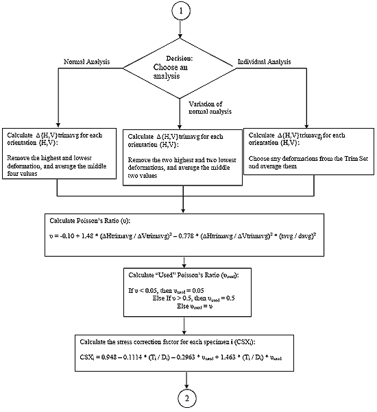
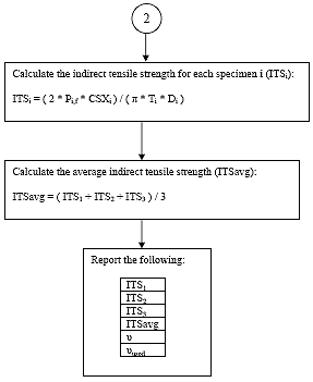
B.4.3.2 Subroutine 1
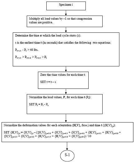
LTPP LABORATORY MATERIAL HANDLING AND TESTING
LABORATORY MATERIAL TEST DATA
CREEP COMPLIANCE, RESILIENT MODULUS AND INDIRECT TENSILE STRENGTH
LAB DATA SHEET T07 - SAMPLE SUMMARY INFORMATION
ASPHALT CONCRETE LAYER (ASPHALTIC CONCRETE PROPERTIES)
LTPP TEST DESIGNATION AC07/LTPP PROTOCOL P07
LABORATORY PERFORMING TEST:___________________________________________________________
LABORATORY IDENTIFICATION CODE: ___ ___ ___ ___
| 1. STATE CODE: ___ ___ | 2. SHRP ID: ___ ___ ___ ___ |
| 3. LAYER NO: ___ | 4. FIELD SET: ___ |
| DATA ITEM | SPECIMEN 1 | SPECIMEN 2 | SPECIMEN 3 |
| 5. TEST NO | ___ | ___ | ___ |
| 6. SAMPLE AREA (SA-) | ___ ___ | ___ ___ | ___ ___ |
| 7. LOCATION NO | __ __ __ __ __ __ | __ __ __ __ __ __ | __ __ __ __ __ __ |
| 8. LTPP SAMPLE NO | __ __ __ __ __ __ __ | __ __ __ __ __ __ __ | __ __ __ __ __ __ __ |
| 9. AVG. THICKNESS (mm) | ___ ___ . ___ | ___ ___ . ___ | ___ ___ . ___ |
| 10. AVG. DIAMETER (mm) | ___ ___ ___ . ___ | ___ ___ ___ . ___ | ___ ___ ___ . ___ |
| 11. BULK SPECIFIC GRAVITY | ___ . ___ ___ ___ | ___ . ___ ___ ___ | ___ . ___ ___ ___ |
| 12. COMMENT 1 | ___ ___ | ___ ___ | ___ ___ |
| 13. COMMENT 2 | ___ ___ | ___ ___ | ___ ___ |
| 14. COMMENT 3 | ___ ___ | ___ ___ | ___ ___ |
| 15. Other Comments |
| 1. STATE CODE: ___ ___ | 2. SHRP ID: ___ ___ ___ ___ |
| 3. LAYER NO: ___ | 4. FIELD SET: ___ |
| DATA ITEM | SPECIMEN 1 | SPECIMEN 2 | SPECIMEN 3 |
| RESILIENT MODULUS TEST | |||
| 16. DATA FILENAME, TEST 1 | _ _ _ _ _ _ _ _ . DAT | _ _ _ _ _ _ _ _ . DAT | _ _ _ _ _ _ _ _ . DAT |
| 17. TEST 1 TEMP. (°C) | ___ ___ . ___ | ___ ___ . ___ | ___ ___ . ___ |
| 18. DATA FILENAME, TEST 2 | _ _ _ _ _ _ _ _ . DAT | _ _ _ _ _ _ _ _ . DAT | _ _ _ _ _ _ _ _ . DAT |
| 19. TEST 2 TEMP. (°C) | ___ ___ . ___ | ___ ___ . ___ | ___ ___ . ___ |
| 20. DATA FILENAME, TEST 3 | _ _ _ _ _ _ _ _ . DAT | _ _ _ _ _ _ _ _ . DAT | _ _ _ _ _ _ _ _ . DAT |
| 21. TEST 3 TEMP. (°C) | ___ ___ . ___ | ___ ___ . ___ | ___ ___ . ___ |
| 22. ANALYSIS FILENAME | _ _ _ _ _ _ _ _ . MRO | ||
| CREEP COMPLIANCE TEST | |||
| 23. DATA FILENAME, TEST 1 | _ _ _ _ _ _ _ _ . DAT | _ _ _ _ _ _ _ _ . DAT | _ _ _ _ _ _ _ _ . DAT |
| 24. TEST 1 TEMP. (°C) | ___ ___ . ___ | ___ ___ . ___ | ___ ___ . ___ |
| 25. DATA FILENAME, TEST 2 | _ _ _ _ _ _ _ _ . DAT | _ _ _ _ _ _ _ _ . DAT | _ _ _ _ _ _ _ _ . DAT |
| 26. TEST 2 TEMP. (°C) | ___ ___ . ___ | ___ ___ . ___ | ___ ___ . ___ |
| 27. DATA FILENAME, TEST 3 | _ _ _ _ _ _ _ _ . DAT | _ _ _ _ _ _ _ _ . DAT | _ _ _ _ _ _ _ _ . DAT |
| 28. TEST 3 TEMP. (°C) | ___ ___ . ___ | ___ ___ . ___ | ___ ___ . ___ |
| 29. ANALYSIS FILENAME | _ _ _ _ _ _ _ _ . OUT | ||
| INDIRECT TENSILE STRENGTH TEST | |||
| 30. DATA FILENAME | _ _ _ _ _ _ _ _ . DAT | _ _ _ _ _ _ _ _ . DAT | _ _ _ _ _ _ _ _ . DAT |
| 31. TEST TEMP. (°C) | ___ ___ . ___ | ___ ___ . ___ | ___ ___ . ___ |
| 32. ".OUT" FILENAME | _ _ _ _ _ _ _ _ . OUT | ||
| 33. ".STR" FILENAME | _ _ _ _ _ _ _ _ . STR | ||
| 34. ".FAM" FILENAME | _ _ _ _ _ _ _ _ . FAM | ||
| GENERAL REMARKS:___________________________________________________________________________ | |
| SUBMITTED BY, DATE | CHECKED AND APPROVED, DATE |
| ______________________________ | ______________________________ |
| LABORATORY CHIEF Affiliation______________________ | Affiliation______________________ |
| << Previous | Contents | Next >> |