U.S. Department of Transportation
Federal Highway Administration
1200 New Jersey Avenue, SE
Washington, DC 20590
202-366-4000
Federal Highway Administration Research and Technology
Coordinating, Developing, and Delivering Highway Transportation Innovations
| REPORT |
| This report is an archived publication and may contain dated technical, contact, and link information |
| Publication Number: FHWA-RD-01-113 Date: October 2002 |
Publication Number: FHWA-RD-01-113 Date: October 2002 |
PDF files can be viewed with the Acrobat® Reader®
Deflection basin measurements have been made with the Falling Weight Deflectometer (FWD) on all test sections that are included in the Long Term Pavement Performance (LTPP) program. These deflection basin data are analyzed to obtain the structural-response characteristics of the pavement structure and subgrade that are needed to achieve the overall LTPP program objectives.
One of the more common methods for analysis of deflection data is to back-calculate the elastic properties for each layer and provide the elastic layer modulus that are typically used for pavement evaluation and rehabilitation design. This report documents the procedure that was used to back-calculate, in mass, the elastic properties for both flexible and rigid pavements in the LTPP program using layered elastic analyses. Obtaining these elastic layer properties for use in further data analyses and studies regarding pavement performance was the primary objective of this study.
T. Paul Teng, P.E.
Director
Office of Infrastructure
Research and Development
Notice
This document is disseminated under the sponsorship of the
U.S. Department of Transportation in the interest of information exchange. The
U.S. Government assumes no liability for the use of the information contained in this document.
The
U.S. Government does not endorse products or manufacturers. Trademarks or manufacturers' names appear in this report only because they are considered essential to the objective of the document.
Quality Assurance Statement
The Federal Highway Administration (FHWA) provides high-quality information to serve Government, industry, and the public in a manner that promotes public understanding. Standards and policies are used to ensure and maximize the quality, objectivity, utility, and integrity of its information. FHWA periodically reviews quality issues and adjusts its programs and processes to ensure continuous quality improvement.
Technical Report Documentation Page
| 1. Report No.
FHWA-RD-01-113 |
2. Government Accession No. | 3 Recipient's Catalog No. | ||
| 4. Title and Subtitle
Back-Calculation of Layer Parameters for LTPP Test Sections, Volume II: Layered Elastic Analysis for Flexible and Rigid Pavements |
5. Report Date OCTOBER 2002 |
|||
| 6. Performing Organization Code | ||||
| 7. Author(s)
H. L. Von Quintus and A. L. Simpson |
8. Performing Organization Report No.
|
|||
|
9. Performing Organization Name and Address Fugro-BRE, 8613 Cross Park Drive, Austin, TX 78754 |
10. Work Unit No. (TRAIS) C6B |
|||
| 11. Contract or Grant No. DTFH61-96-C-00003 | ||||
| 12. Sponsoring Agency Name and Address
Office of Engineering R & D Federal Highway Administration, 6300 Georgetown Pike, McLean, Virginia 22101-2296 |
13. Type of Report and Period Covered
Final Report, May 1997 -- August 2001 |
|||
|
14. Sponsoring Agency Code HCP 30-C |
||||
| 15. Supplementary Notes This report is a project deliverable under the LTPP Data Analysis Technical Support study. ERES Consultants is the prime contractor, and Fugro-BRE is a subcontractor. Fugro-BRE staff members who provided significant contributions to this study include Dr. Peter Jordahl and Mr. Dale Framelli. Contracting Officer's Technical Representative (COTR): Cheryl Allen Richter, HRDI-13 | ||||
| 16. Abstract
This report documents the procedure and steps used to back-calculate the layered elastic properties (Young's modulus and the coefficient and exponent of the nonlinear constitutive equation) from deflection basin measurements for all of the LTPP test sections with a level E data status. The back-calculation process was completed with MDOCOMP4 for both flexible and rigid pavement test sections in the LTPP program. The report summarizes the reasons why MODCOMP4 was selected for the computations and analyses of the deflection data, provides a summary of the results using the linear elastic module (Young's modulus) for selected test sections, and identifies those factors that can have a significant effect on the results. Results from this study do provide elastic layer properties that are consistent with previous experience and laboratory material studies related to the effect of temperature, stress-state, and season on material load-response behavior. In fact, over 75 percent of the deflection basins analyzed with the linear elastic module of MODCOMP4 resulted in solutions with an RMS error less than 2.5 percent. Those pavements exhibiting deflection-softening behavior with Type II deflections basins were the most difficult to analyze and were generally found to have RMS errors greater than 2 percent. In summary, the nonlinear module of MODCOMP did not significantly improve on the number of reasonable solutions, and it is recommended that nonlinear constitutive equations not be used in a batch mode basis. |
||||
| 17. Key Words
MODCOMP, Back-Calculation, Modulus, Young's Modulus, Elastic Properties, Surface Deflection, Stress Sensitivity. |
18. Distribution Statement
No restrictions. This document is available to the public through the National Technical Information Service, Springfield, VA 22161. |
|||
|
19. Security Classification Unclassified |
20. Security Classification Unclassified |
21. No. of Pages 144 |
22. Price | |
| Form DOT F 1700.7 | Reproduction of completed page authorized |
SI* (Modern Metric) Conversion Factors
2.0 SELECTION OF BACK-CALCULATION METHODOLOGY
4.0 RESULTS FROM COMPUTATION OF ELASTIC PROPERTIES
5.0 SUMMARY OF FINDINGS AND RECOMMENDATIONS
APPENDIX A.0: Back-Calculation of Layer Elastic Properties from LTPP-FWD Deflection Basin
APPENDIX B.0: Test Section Classification and Subgrade Information for the Back-Calculation Process
APPENDIX C: Median Values and Histograms of Young's Modulus Back-Calculated for Different Materials
Deflection basin measurements have been made with the Falling Weight Deflectometer (FWD) on all General Pavement Study (GPS) and Specific Pavement Study (SPS) test sections that are included in the Long-Term Pavement Performance (LTPP) program. This deflection-testing program is being conducted periodically to obtain the load-response characteristics of the pavement structure and subgrade. FWD deflection basin tests are conducted about every 2 years for the SPS project sites and about every 5 years for the GPS sites. There are 64 test sections included in the LTPP Seasonal Monitoring Program (SMP), and these sites are tested about every month over a period of 1 to 2 years. These deflection basin data are intended to provide structural-response characteristics that are needed to achieve the overall LTPP program objectives.
One of the more common methods for analysis of deflection data is to back-calculate the elastic properties for each layer in the pavement structure and foundation. These analysis methods (referred to as back-calculation programs) provide the elastic layer modulus typically used for pavement evaluation and rehabilitation design. At present, interpretation of deflection basin test results usually is performed with static-linear analyses, and there are numerous computer programs that can be used to calculate these elastic modulus values (Young's modulus).
This report documents the procedure that was used to back-calculate, in mass, the elastic properties for both flexible and rigid pavements in the LTPP program using layered elastic analyses. All data used for this back-calculation study were extracted from the LTPP data release dated October 1997 for the SMP sites and April 1998 for the GPS and SPS sites, and have a level E status (the highest quality data in the LTPP database). All work was completed under the LTPP Data Analysis Technical Support Study (Contract No. DTFH61-96-C-00003).
1.2 LTPP Deflection Testing Program
The LTPP deflection basin testing program uses seven sensors placed at 0, 203, 305, 457, 610, 914, and 1524 mm from the center of the load plate to define the shape of the deflection basin. The loading sequence, as stored in the LTPP database for flexible and rigid pavement testing, is summarized in table 1. The following summarizes the general locations for the deflection tests for each different type of pavement.
| Pavement Type | Drop Height | Number of Drops | Target Load, kN | Acceptable Load Range, kN |
|---|---|---|---|---|
| Flexible | 3 | 3 | Seating | --- |
| Flexible | 1 | 4 | 26.7 | 24.0 to 29.4 |
| Flexible | 2 | 4 | 40.0 | 36.0 to 44.0 |
| Flexible | 3 | 4 | 53.4 | 48.1 to 58.7 |
| Flexible | 4 | 4 | 71.2 | 64.1 to 78.3 |
| Rigid, JCP & CRCP | 3 | 3 | Seating | --- |
| Rigid, JCP & CRCP | 2 | 4 | 40.0 | 36.0 to 44.0 |
| Rigid, JCP & CRCP | 3 | 4 | 53.4 | 48.1 to 58.7 |
| Rigid, JCP & CRCP | 4 | 4 | 71.2 | 64.1 to 78.3 |
A more complete description of the testing plan and data storage in the database is provided in LTPP Manual for Falling Weight Deflectometer Measurements -- Operational Field Guidelines, Version 3.1, dated August 2000.
The primary objective of this study was to back-calculate the elastic layer properties from deflection basin measurements for use in further data analyses and studies regarding pavement performance. As part of this objective, the elastic layer properties back-calculated from the deflection basin data for the LTPP flexible and rigid pavement test sections were to be included in the LTPP computed parameter database for future use.
A secondary objective of this study was to provide any modifications to the current guidelines that have been prepared for use in back-calculating elastic properties. These guidelines include ASTM D5858 and the procedure written by Von Quintus and Killingsworth.(1) Another secondary objective was to identify those LTPP test sections with unusual load-response characteristics.
1.4 Application of Results to Future Studies
The elastic properties computed for each structural layer in the pavement structure and subgrade strata can be used in future studies of materials-pavement behavior and performance. In fact, these computed parameters will be needed to achieve some of the stated objectives and "outcomes" identified in the LTPP Strategic Plan that was published in 1999.(18) For example, elastic properties can be used directly in developing or validating load-related distress prediction models based on elastic layer theory or used indirectly for selecting test sections with significantly different properties for studying a particular design issue. The following lists some of the LTPP strategic objectives where the results from this study can be used to achieve those objectives.
Some specific applications of these results are listed below.
There are three basic approaches to back-calculating layered elastic moduli of pavement structures: 1) the equivalent thickness method (e.g., ELMOD and BOUSDEF), 2) the optimization method (e.g., MODULUS and WESDEF), and 3) the iterative method (e.g., MODCOMP and EVERCALC). Layer thickness is a critical parameter that must be accurately known for nearly all back-calculation programs, regardless of methodology, although some programs claim to be able to determine a limited set of both Young's modulus and layer thickness (e.g., MICHBACK).(2) Many of the software packages are similar, but the results can be different as a result of the assumptions, iteration technique, back-calculation, or forward-calculation schemes used within the programs.
Within the past couple of decades, there have been extensive efforts devoted to improving back-calculation of elastic-layer modulus by reducing the absolute error or root mean squared (RMS) error (difference between measured and calculated deflection basins) to values as small as possible. The absolute error term is the absolute difference between the measured and computed deflection basins expressed as a percent error or difference per sensor; whereas the RMS error term represents the goodness-of-fit between the measured and computed deflection basins.
The use of these linear elastic layer programs, however, has been only partly successful in analyzing the deflections measured at the LTPP sites. For example, only about 50 percent of the flexible GPS sites were found to have absolute error terms less than the generally considered reasonable value of 2 percent per sensor.(3,4) In addition, results from use of linear elastic models are highly variable, with an undefined reliability over a wide range of conditions.
So the question is: which program should be used to back-calculate Young's modulus for each structural layer in the pavement structure?
The purpose of this section is to document the methodology and software package used for back-calculating pavement layer and subgrade moduli from the deflection basins measured on all LTPP test sections that have a level E data status.
The common analysis method is to back-calculate material response parameters for each layer within the pavement structure from the FWD deflection basin measurements. Many of the back-calculation programs are limited by the number and thickness of the layers used to define the pavement structure but, more importantly, assume that the layers are linear elastic. Most unbound pavement materials and soils are nonlinear. Thus, the calculated layer-modulus represents an "effective" Young's modulus that adjusts for stress-sensitivity and discontinuities or anomalies (such as variations in layer thickness, localized segregation, cracks, and the combinations of similar materials into a single layer).
The back-calculation methods can be grouped into four general categories.
2.1.1 Type of Load Application. At present, interpretation of deflection basin test results is performed with static analyses. There have been many improvements in back-calculation technology within the past 4 to 5 years. These improvements have spawned standardization procedures and guidelines to ensure that there is consistency within the industry and to improve upon the load-response characterization of the pavement structural layers.(5) ASTM D5858 is a procedure for analyzing deflection basin test results to determine layer elastic moduli (i.e., Young's modulus).
There are no similar standardized procedures for back-calculating materials properties of pavement layers using dynamic analysis techniques. In fact, there are only a few programs that have the capability to do dynamic analyses. Thus, the programs using dynamic analyses were not considered for use in calculating elastic-layer modulus from hundreds of deflection basins measured at the same site. Only the static load application analysis methods were considered appropriate for use in a production mode -- mass back-calculation of elastic layer modulus from deflection basins measured along the LTPP test sections.
2.1.2 Type of Material Response Models. Most of the back-calculation procedures that have been used to determine layer moduli are based on elastic layer theory. However, some of the programs based on elastic theory have been modified to account for the viscoelastic (time-dependent) or elastoplastic (inelastic) behavior of materials. Unfortunately, programs that include time-dependent properties or inelastic properties have not been used in a production mode and, more importantly, have not been very successful in producing consistent and reliable solutions.
SHRP, as well as others, studied and evaluated many of these back-calculation procedures to select one method for use in characterizing the subgrade and other pavement layers in order to predict the performance of flexible and rigid pavements.(6,7) The program entitled "MODULUS 4.0" was selected for flexible and composite pavements, whereas a new procedure was developed for rigid pavements as part of the SHRP P-020 Data Analysis Project.(8,9) As stated above, many of these programs are limited by the following:
Thus, it must be understood that the calculated layer modulus represents an "effective" or "equivalent" elastic modulus that accounts for differences in stress states and any discontinuities or anomalies (such as variations in layer thickness, slippage between two adjacent layers, cracks, and the combinations of similar materials into a single layer).
Although there have been extensive efforts devoted to improving back-calculation of layer moduli by reducing the RMS error to values as small as possible, highly variable results from the use of linear elastic models have been found with an undefined reliability over a wide range of conditions. In addition, models that assume a linear response of materials require numerous iterations at varying load levels (different drop heights) to identify the stress sensitivity of unbound pavement materials and soils. From this standpoint, the use of nonlinear elastic layer programs was believed to have merit.
Two programs that have been used with some success and contain a nonlinear structural response capability are MODCOMP and a program developed by the Corps of Engineers at the Waterways Experiment Station.(10,11) The Corps of Engineers program has the capability of a true nonlinear response model but has not been used on a large number of projects and does not have a batch mode processor or data management software to facilitate its use in a production mode. Conversely, MODCOMP can be used on a production mode basis, and its convergence is reasonably fast, but it is a quasi-nonlinear response model. Stated differently, for the same load level, the modulus of a layer does not vary horizontally or vertically within that layer in accordance with changes in stress state. The layer modulus is only varied by stress state between load levels and sensor locations.
Standardized procedures and guidelines are available to assist in this back-calculation process. Some of these include procedures written under the SHRP program ASTM D5858 and the one documented in report FHWA-RD-97-076, Design Pamphlet for the Back-Calculation of Pavement Layer Moduli in Support of the 1993 AASHTO Guide for the Design of Pavement Structures.(1,5,6) All of these programs and guidelines are based on the use of elastic layer response programs. Viscoelastic or elastoplastic response programs have not been used in a sufficient number of projects to substantiate the reliability and adequacy of their use. Therefore, selection of the back-calculation software and procedures were confined to those that are based on the use of elastic layer theory.
2.1.3 Summary. Although many analyses of deflection data can be undertaken, the studies currently underway within the LTPP program, by definition, require highly focused efforts accomplishable within a short period of time. Thus, the study for back-calculating layer moduli looked only at the computation of material properties using existing software that has the capability to analyze massive amounts of deflection data in a reasonable time frame. These requirements basically restrict the back-calculation methodology to a static load analyzed with a linear or nonlinear elastic response model.
It should be understood that many different software packages can be used to calculate the elastic modulus of pavement layers and subgrade soils from deflection basins, as demonstrated in report FHWA-RD-97-086, Back-Calculation of Layer Moduli of LTPP GPS Sites.(3) Many of the software packages that have the same type of response model have, in fact, provided reasonably consistent results. The following lists the factors considered for evaluating the different back-calculation programs based on elastic layer theory and were found to be applicable to pavement diagnostic studies and the requirements noted above.
2.3 Selection of Software -- MODCOMP4
The evaluation focused on two areas: (1) the ability and accuracy of the software to determine elastic-layer moduli of the pavement materials and soils and (2) operational characteristics -- ease of use mode, flexibility in analyzing a wide range of pavement structures (flexible and rigid), and material response models. Much of the information used for the software selection process was obtained from previous comparisons and evaluation studies of the software. (See references 3, 7, 12, and 13.)
The primary reasons that MODCOMP4 was selected as the program for calculating the elastic properties of pavement structural layers and subgrade soils from FWD deflection basins measured at the LTPP SMP, GPS, and SPS test sections are listed below.
One of the most difficult questions to be answered is, How accurate are the layer moduli back-calculated from measured deflection basins? In reality, this is an impossible question to answer conclusively for real basins, but it must be addressed to promote confidence in the computed results. This section describes the procedure used to estimate the accuracy of the results.
A small experiment was conducted to check out the capabilities of MODCOMP using LTPP data and the procedure used for classifying deflection data in terms of load response patterns and deflection basin shapes.(1,4) Elastic layer theory (specifically, ELSYM5)1 was used to calculate a deflection basin under a specific load and a known set of layer moduli. The computed deflection basin was considered a measured basin and input into MODCOMP. The program was then used to back-calculate the layer moduli for each layer.
Note: 1ELSYM5 Version 1.1 , corrected in 1993, was the version used for these calculations.
These calculated layer moduli were compared to the known values that were originally used to calculate the deflection basin. The differences between the calculated and target (or known) moduli were used to estimate the accuracy of the program and to establish a practical error term for the matched deflection basins. This is a process that has been used previously by the authors in evaluating the results from other back-calculation programs.
To perform this preliminary analysis, only the linear elastic layer portion of the MODCOMP4 program was used. The nonlinear part was not included in this part of the study. A factorial was developed to cover the expected range of the conditions and pavement structures that are included in the LTPP database. Table 2 shows the factorial that was used for this effort.
Back-calculation was conducted only for those cells where an "X" appears in the factorial (see table 2). These cells were selected because they represented the extreme conditions. The stiffer layer for the "inverted pavements" was established as an asphalt-treated base, 25.4 centimeters in thickness, with an elastic modulus of either 689 MPa or 13,790 MPa. The unbound granular bases for the "conventional pavements" were all 25.4 centimeters in thickness and had an elastic modulus of 2,007 MPa.
of the MODCOMP4 solutions.
| Type of Pavement |
Subgrade Strength |
Depth To A Rigid Layer |
Surface Layer: Moduli, ksi, 6,895 MPa; Thickness 15.2 cm |
Surface Layer: Moduli, ksi, 6,895 MPa; Thickness 7.6 cm |
Surface Layer: Moduli, ksi, 2069 MPa; Thickness 15.2 cm |
Surface Layer: Moduli, ksi, 2069 MPa; Thickness 7.6 cm |
|---|---|---|---|---|---|---|
| Conventional | Strong, 207 MPa | Infinite | X | |||
| Conventional | Strong, 207 MPa | Shallow, 1.8 m | X | |||
| Conventional | Weak, 69 MPa | Infinite | X | X | ||
| Conventional | Weak, 69 MPa | Shallow, 1.8 m | X | X | ||
| Inverted1 | Strong, 207 MPa | Infinite | X | X | X | |
| Inverted1 | Strong, 207 MPa | Shallow, 1.8 m | ||||
| Inverted1 | Weak, 69 MPa | Infinite | X | |||
| Inverted1 | Weak, 69 MPa | Shallow 1.8 m | X | X |
1Inverted, in this case, means a pavement with a stiffer layer (higher modulus material below or supporting a weaker material in the pavement structure).
The RMS error for each solution and the percent difference between the calculated modulus and the target modulus were the study results considered in the evaluation. The RMS error was found to vary from 0.1 to 1 percent, which is considered very acceptable. The following are the average and standard deviations of the RMS error.
Accuracy of the computed results was found to vary with layer depth, which has been observed in other studies. The following summarizes the differences (percent of the target value) as a function of layer within the pavement structures.
| Layer | Back-Calculated E/Target E Mean | Back-Calculated E/Target E Mean Standard Deviation |
|---|---|---|
| Surface (7.6 or 15.2 cm in thickness) | 1.191 | 0.5877 |
| Stabilized Base Layers | 1.101 | 0.3427 |
| Unbound Granular Base/Subbase Layers | 1.078 | 0.2322 |
| Subgrade Layers | 1.008 | 0.0420 |
As shown above, on the average, the back-calculated layer moduli are slightly greater than the target or known values used to calculate the deflection basins. In summary, use of linear elastic back-calculation programs may result in errors on the order of 20 percent for surface layers, 10 percent for stabilized base or subbase layers, 8 percent for unbound granular base/subbase layers, and 1 percent for subgrades.
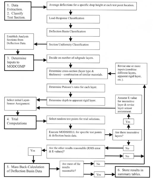
The process that was used to back-calculate the elastic properties of the pavement layers and subgrade soils are summarized in this part of the report. The overall operational process follows the procedure outlined by Von Quintus and Killingsworth in publication FHWA-RD-97-076 and the Instructional Guide for Back-Calculation and the Use of MODCOMP.(1,10) Appendix A of this report is the User's Guide, which defines all of the steps, programs and decision functions included in this process. Figure 1 shows a simplified flow chart of the major steps and decisions used in the back-calculation process. As shown, there are six major steps:
This section of the report discusses and defines three of the six steps in more detail than in appendix A -- Test Section Classification, Determination of Inputs, and Trial Computations.
3.1 Test Section Classification
The deflection data measured at each site were used to classify the test sections with similar deflection characteristics. Three deflection-site classifications were used: (1) a load-response classification, (2) a deflection basin classification, and (3) a test section uniformity classification. Each is defined in the following paragraphs.
3.1.1 Load-Response Classification. The first step in the test section classification was to determine the load-response characteristics of the pavement structures included in the LTPP database. In general, there are three types of load-response categories:
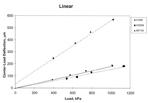
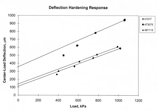
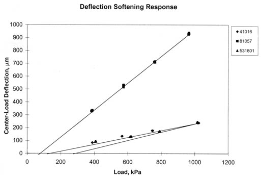
In determining the load-response behavior of these test sections, a linear model was used (i.e., a linear relationship between load and the deflection measured at the center of the loading plate). The slope and intercept were determined for each set of deflection data, and the multiple correlation coefficient, R2, was determined for these linear relationships for each set of deflection data. The criteria used to characterize the load-response behavior was somewhat judgmental, but was defined by R2 and the deflection intercept plus geometric considerations. The criteria used to establish the load-response behavior are listed below.
Although the intercept values are arbitrary, the plot must go through the origin for zero-load so that the shape of the response curve is determined. If deflection decreases with load, deflection hardening must be occurring in one or more layers. Conversely, deflection increases with increasing loads indicate deflection softening.
It should be noted that the initial characterization for categorizing the GPS test sections was based only on the center-load deflections. A more complete subdivision of the sections would use some of the other deflections measured at specific radial distances from the load plate (for example, 305, 610, and 1,524 mm). This would help in selecting different constitutive equations to be used for different layers and material types. The majority of the LTPP tests sections were found to have linear elastic load-deflection response characteristic; very few of the sections exhibit deflection-softening behavior, as expected.
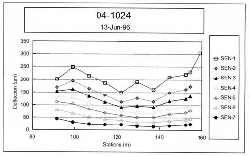
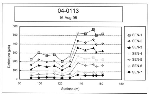
3.1.2 Deflection Basin Classification. To evaluate the different types of deflection basins, all measured basins were first normalized to the center-load deflection, which is directly under the load. These normalized deflection basin data were divided into four types of basins. This is the same procedure followed by Von Quintus, et al., as documented in report FHWA-RD-97-076.(1) Examples of basins for these different categories are shown in figures 5-8 and defined below:
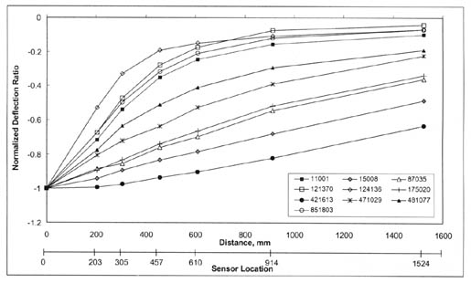
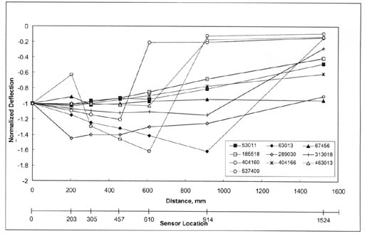
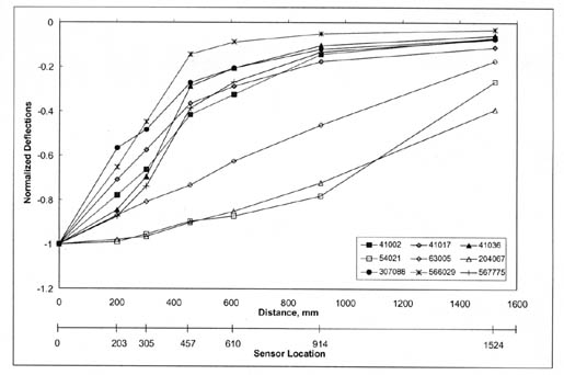
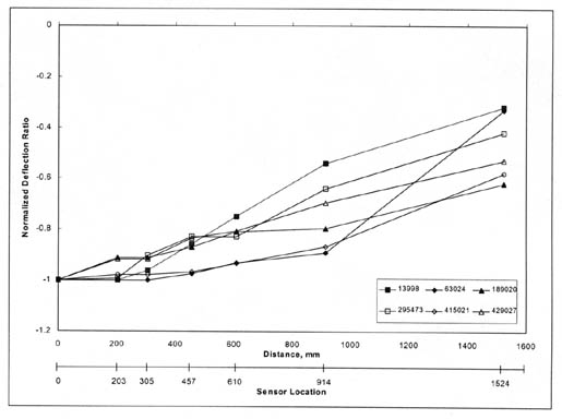
In general, Type I and III deflection basins occur most frequently for PCC surfaced pavements. It is believed that these deflection basins may be characteristic of those areas with voids, a loss of support, a severe thermal gradient causing curling of the PCC slab, and/or a combination of these conditions. Conversely, Type II deflection basins occur most frequently for dense-graded asphalt concrete surfaced pavements. As stated above, all Type I and III basins were excluded from the actual back-calculation process.
3.1.3 Test Section Uniformity Classification. The final step included in the classification of each LTPP test section was to determine the uniformity or variability of the deflections measured along the test section. The uniformity of each LTPP test section was classified into one of four different categories, listed below.
The site-uniformity characterization defines whether the test section can be considered initially as one uniform section or whether the test section should be treated as multiple sections. Appendix B of this report lists those LTPP test sections that were subdivided into two subsections.
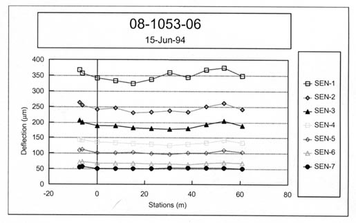
Those test sections with significant differences in the load response between the ends of the test sections (figure 12) were flagged and subdivided into two subsections. The pavement layer thickness was then checked to determine whether different layer thicknesses or material types exist between the two ends of the section. If significant differences were found to exist, that section was subdivided based on the differences in the deflection data.
Appendix A provides a detailed discussion on determination of the inputs to MODCOMP4 for each test section. Table 3 summarizes the sources for the input data needed for the back-calculation of layer modulus from deflection basin data for the LTPP sites. The following paragraphs overview some of the more important input issues.
| Input Parameter | Data Source or Table | Remarks |
|---|---|---|
| Deflection Basins | MON_DEFL_DROP_ DATA |
Average deflection basin for each drop height and test point. |
| Pavement Temperature | MON_DEFL_TEMP_ VALUES_DEPTH |
Mid-depth temperatures used to calculate the seed modulus of HMA layers using the dynamic modulus equation.(15) |
| Pavement Cross-Section, Material Type and Layer Thickness | TST_L05B | The pavement cross-section used to back-calculate layer modulus. |
| Pavement Cross-Section, Material Type and Layer Thickness | TST_L05A | The pavement cross-section used to back-calculate layer modulus. |
| Asphalt Viscosity | INV_PMA_ASPHALT | Data elements needed in the dynamic modulus equation. |
| HMA Aggregate Gradation | TST_AG04 | Data elements needed in the dynamic modulus equation. |
| HMA Aggregate Gradation | INV_GRADATION | Data elements needed in the dynamic modulus equation. |
| Air Voids | TST_AC02 | Data elements needed in the dynamic modulus equation. |
| Air Voids | TST_AC03 | Data elements needed in the dynamic modulus equation. |
| Air Voids | INV_PMA_ORIG_MIX | Data elements needed in the dynamic modulus equation. |
| Density, HMA and ATB | TST_AC02 | Data elements needed to estimate overburden pressure -- nonlinear solutions. |
| Density, Unbound Layers and Soils | TST_ISD_MOIST | Data elements needed to estimate overburden pressure -- nonlinear solutions. |
| Number of Subgrade Layers | TST_SAMPLE_LOG | Data element used to subdivide subgrade. |
| Depth to Water Table | TST_SAMPLE_LOG | Data element needed to subdivide subgrade. |
| Depth to Apparent Rigid Layer | TST_SAMPLE_LOG | |
| Poisson's Ratio | Table 4 | Default values. |
| Lateral Earth Pressure Coefficient | Table 4 | Default values -- nonlinear solutions. |
A few pavements were studied using two measured basins at each load level versus using the average of the measured basins at each load level. Based on the limited comparisons completed, use of the average deflection basin at each drop height provided back-calculated moduli comparable to those averaged from separate back-calculations for each basin. The differences were generally within the simulation error previously discussed.
3.2.2 Pavement Cross-Section. All layer thickness and material types were extracted from data tables TST_L05B or TST_L05A in the Information Management System (IMS) database. The initial pavement cross-section (combination of pavement layers and subgrade soil stratas) used in the back-calculation process was obtained from previous work completed by Von Quintus and Killingsworth.(3) When the material types and/or layer thicknesses for the approach and leave ends of a test section were significantly different, as defined in Appendix A, that test section was flagged and put aside for further review. The longitudinal variation in the deflection basin data was reviewed carefully to subdivide the test section into two segments with different cross-sections, as noted above.
3.2.3 Material Properties and Temperatures. Various material properties and the temperature during FWD testing were extracted from different data tables in the database. These data were used to calculate the starting or "seed" modulus of the hot mix asphalt (HMA) layers for the linear solutions using the Witczak dynamic modulus regression equation.(15) The mid-depth temperatures during FWD testing were extracted from data table MON_DEFL_TEMP_VALUES_DEPTHS. The material properties were extracted from data tables INV_PMA_ASPHALT (asphalt viscosity), TST_AG04 or INV_GRADATION (gradation), and TST_AC02 and TST_AC03 (bulk and Rice specific gravities to calculate air voids) or INV_PMA_ORIG_MIX (air voids).
3.2.4 Layer-Sensor Assignment. MODCOMP assigns specific sensors to certain layers. Initially, the default layer-sensor assignment was used. In many cases (10 to 25 percent of the test sections), however, the initial layer-sensor assignments were changed manually to reduce the RMS error. One of the primary reasons for changing the automatic layer-sensor assignments was that the computed deflection basin was insensitive to a specific layer. For those cases, Young's modulus was simply assumed for the insensitive layer, and the sensor was reassigned to an adjacent layer. The assumed value or modulus was based on the initial computations and previous laboratory test results for similar materials.
3.2.5 Poisson's Ratio. Poisson's ratio is not available in the LTPP database. This material property was assumed for each type of material and based on previous guidelines. The values of Poisson's ratio, used for different materials and soils, are given in table 4.
3.2.6 Multiple Subgrade Layers. A 6-m boring was drilled adjacent to the pavement at all LTPP sites. This boring is defined as a shoulder probe and used to identify the different soil strata and determine the depth to a rigid layer and water table. The soil profile obtained from the 6-m shoulder probe was used to identify whether the subgrade should be divided into two or more layers, and if so, at what depth. The shoulder probes were obtained from data table TST_SAMPLE_LOG in the IMS. In general, the subgrade was divided into multiple layers when the following conditions were found: (1) significantly different soils were encountered, (2) water or very wet soils were encountered, and (3) extremely stiff or hard soils were noted on the boring log.
3.2.7 Depth to an Apparent Rigid Layer. The soil profile or shoulder probe boring also was used to determine the depth to an apparent rigid layer, and this depth was compared to the calculated depth using the latest revision of MODULUS.(16) In many cases, lower RMS errors were calculated when no apparent rigid layer was used in the back-calculation process. The depth to an apparent rigid layer was kept constant when that depth was determined from the boring log. Appendix B identifies when a rigid layer was used and at what depth for the test section.
3.2.8 Constitutive Equation. MODCOMP4 has the capability to consider different constitutive equations to model the response of the pavement materials and subgrade soils. These constitutive equations are summarized in table 5. Each has been used with some degree of success, and the results from a previous study indicate that the constitutive model used has a definite influence on the results. Obviously, it is desirable to use the same model for all unbound pavement materials and subgrade soils so that the results can be compared across the board. Unfortunately, none of the models used consistently converged to an acceptable solution for all pavements included in this study.
The bulk stress and minor principal stress models (refer to table 5) appear to be appropriate for use for both fine-grained and coarse-grained materials converged with fewer iterations and resulted in lower RMS errors. The second stress invariant, vertical stress, and major principal stress models (refer to table 5) were abandoned because of the number of solutions that did not converge when these equations were used. Where convergence was not achieved, different constitutive equations were used in follow-on computations to achieve more desirable results. The octahedral shear stress and Cornell constitutive models were not used.
The constitutive equation recommended for use by Von Quintus from a previous study (defined as the so-called Universal Model) uses three parameters, or k-values.(4) That model is unavailable in MODCOMP, and there is an insufficient number of sensors in the LTPP database to support its use to calculate nonlinear elastic properties. Thus, the two equations referred to in the AASHTO Design Guide (the bulk stress and deviator stress models) were used for the first set of runs.(17) The bulk stress model was used for coarse-grained soils, and the deviator stress model was used for fine-grained soils. The minor principal stress model was used in the back-calculation process when the first two did not result in any solution. These three equations are listed below and in table 5.
| Material Description | Material Code | Median Wet Density, pcf | Median Dry Density, pcf | Percent Median Moisture Content | Poisson's Ratio | At-Rest Earth Pressure Coefficient |
|---|---|---|---|---|---|---|
| Cohesive Soil: High Plasticity Clay Soils | 101-137 | 129 | 109 | 18.3 | Soft 0.45, Stiff 0.40, Hard 0.30, (0.30 - 0.48) | Soft 0.80, Stiff 0.70, Hard 1.00 |
| Cohesive Soil: Low Plasticity Clay Soils | 101-137 | 129 | 109 | 18.3 | Soft 0.45, Stiff 0.40, Hard 0.40, (0.30 - 0.48) | Soft 0.80, Stiff 0.70, Hard 1.00 |
| Silty Soils | 141-148 | 130 | 113 | 15.4 | Above Water Table 0.35, Below Water Table 0.40, (0.30 - 0.45) | Above Water Table 0.70, Below Water Table 0.70 |
| Sandy Soils | 201-217 | 129 | 116 | 10.7 | Above Water Table 0.35, Below Water Table 0.40, (0.20 - 0.40) | Above Water Table 0.60, Below Water Table 0.80 |
| Gravelly Soils | 251 - 267 | 137 | 123 | 9.6 | 0.35 | 0.50 |
| Lime Treated Soils | 338 | 124 | 100 | 24.3 | Percent Lime >4 0.30, Percent Lime < 40.35, (0.20 - 0.40) | * |
| Sand Base | 306-309 | 132 | 124 | 5.8 | 0.35 (0.20 - 0.40) | 0.70 |
| Gravel Base and Crushed Stone Base | 302-305, 337 | 136 | 129 | 5.2 | 0.35 (0.20 - 0.40), 0.30 (0.20 - 0.40) | 0.60, 0.50 |
| Asphalt Treated Base | 321-330 | 118 | --- | --- | Temp: <40°F 0.25, Temp: 40-100°F 0.30, Temp: >100°F 0.35, (0.20 - 0.40) | * |
| Cement Treated Base | 331-335 | 125 | --- | --- | 0.20 (0.15 - 0.25) | * |
| Asphalt Concrete Mixtures (Surface, Bases) | --- | --- | --- | Temp: <40°F 0.25, Temp: 40-100°F 0.30, Temp: >100°F 0.40, (0.15 - 0.45) | * |
| Model | Description |
|---|---|
| 0 | Linear model of the form E = constant. In general, most asphalt concrete, Portland cement concrete, and treated (i.e., stabilized) soil materials conform to this constitutive relationship. |
| 1 | Bulk stress model of the semi-logarithmic form E = k1 exp (S*k2), where
S = Theta = Sigmaz + Sigmat + Sigmar (Sigmaz = vertical stress, Sigmat = tangential stress, and Sigmar = radial stress at the mid-depth of the layer). The parameter Theta is known as the bulk stress or as the first stress invariant. It was originally developed as a log-log model, but since Theta can be either positive or negative, it works better as a semi-log model. It is used for untreated, coarse-grained base and subbase gravels. In terms of overall usage, the bulk stress model is one of the most popular and most commonly used models. |
| 2 | Deviator stress model of the semi-logarithmic form E = k1 exp (S*k2), where
S = Theta = Sigma1 - Sigma2 the difference between the major principal stress and the minor principal stress at the mid-depth of the layer. It can be used for fine-grained untreated materials. Although this model differs from the traditional linear deviator stress model (E = k1S + k2), it seems to work very well. |
| 3 | Minor principal stress model of the semi-logarithmic form E = k1 exp (S*k2), where
S = Sigma3 The parameter Sigma3 is the minor principal stress, which can either be tensile (negative) or compressive (positive). Also known as the "confining stress model," the Sigma3 model was commonly used before the bulk stress model was conceived. It was originally developed as a log-log model, but since Sigma3 can be either positive or negative, it works better as a semi-log model. It can be used for coarse-grained, untreated materials. |
| 4 | Second stress invariant model of the semi-logarithmic form E = k1 exp (S*k2), where
S = J2/(1 + Tauoct) The parameter J2 is the second stress invariant. J2 = Sigmaz Sigmat + Sigmat Sigmar + Sigmat Sigmaz + Taurz2 Where Sigmaz, Sigmat and Sigmar are as defined in Model 1, and Taurz is the shear stress in the rz plane, Tauoct is the octahedral shear stress, which is similar to a root-mean-square deviator stress. Tauoct = Alpha[(Sigmaz - Sigmat)3 + (Sigmat - Sigmar)2 + (Sigmar - Sigmaz)2 + 6 Taurz2]½ This constitutive relationship has been found to be useful for both base course and subgrade materials, and the coefficient k1 appears to be primarily a function of material density and soil moisture tension. It was originally developed as a log-log model, but since J2 can be negative it works better as a semi-log model. |
| 5 | Octahedral shear stress model of the semi-logarithmic form E = k1 exp (S*k2), where
S = (1 + Tauoct) This relationship has been found to be useful for fine-grained materials and for frozen soils, and the coefficient k1 appears to be a function of soil temperature and moisture content. It was originally developed as a log-log model but since toct can be negative, it works better as a semi-log model. |
| 6 | Vertical stress model of the log-log form E = k1 S k2, where
S = Sigmaz The parameter Sigmaz is the vertical stress, which is always compressive (i.e., positive). This model is very similar in some respects to Model 7. The difference is that the direction of Sigmaz is always vertical, while the direction of Sigma1 in Model 7 rotates with distance from the load. |
| 7 | Major principal stress model of the log-log form E = k1 S k2 (k0)k3, where
S = Sigma1 The parameter Sigma1 is the major principal stress, which is generally always compressive. Dynatest uses this model in their ELMOD back-calculation program. It is included here for completeness. As used in ELMOD, the overburden stress is not included in the major principal stress, so the overburden stress is not included in MODCOMP3 either. |
| 8 | Cornell constitutive model of the log-log form E = k1 S k2 (k0)k3, where
S = (Thetao2 + Thetap2)0.22(1-P200) (1 + Tauoct)-0.34P200 The parameter Thetao is the initial bulk stress, due only to overburden stress. The parameter Thetap is the bulk stress at peak load, including both the overburden stress and the load stress. The parameter Tauoct is the octahedral shear stress at peak load, which also includes the overburden stress. The parameter P200 is the percentage of the materials gradation that passes the number 200 sieve, and it is a required input for both known and unknown models. It is entered on data file line 5 as the K@(I) parameter (see Table 3 of the MODCOMP User's Manual). The parameter k0 is the lateral earth pressure coefficient, which represents the anisotropy of the overburden stress. The coefficient k1 has been found to be a function of material density and soil moisture content, along with other material properties. The exponent k3 = -0.69, is treated as a constant in the program. The Cornell model has been developed for use with both coarse-grained and fine-grained untreated materials. It has seen limited use, mainly with the glacial materials of the Northeastern U.S. |
3.2.9 Material Densities. Wet and dry densities for the pavement layers and subgrade are included in the LTPP database for many of the test sections and were extracted from data table TST_ISD_MOIST. When the densities were available, they were used in the back-calculation process. However, when the densities were unavailable for a specific layer and site, the median density for that type of material, calculated from all other data, was used. These default values are listed in table 4.
3.2.10 Lateral Earth Pressure. MODCOMP has the capability to consider the effect of overburden pressures in back-calculating nonlinear elastic properties. The lateral earth pressure coefficient (Ko) is used to compute the contribution to the lateral stress at different depths from the overburden pressure. Lateral earth pressure coefficients, however, are not included in the LTPP database. A range of basins with varying conditions was used to evaluate the sensitivity of Ko to obtain reasonable solutions (low RMS error). For reasonable variations (plus or minus 25 percent) around the default values included in MODCOMP, it was found that Ko does not have a significant effect on the calculated results. Because there is no reliable method to estimate the actual Ko value to be used for each section, the values given in table 4 were used and are materials dependent. For a linear elastic solution, Ko has no effect on the back-calculated moduli.
3.3 Trial Computations -- Execution of Back-Calculation Process
The procedure used to back-calculate the elastic properties of each layer is not fully automated but is an iterative process and requires engineering judgment. To begin the computation process, a limited number of points are randomly selected along the test section and the elastic properties calculated for those basins. The reason for starting with a limited number of basins is to make any necessary revisions to the inputs for reducing the RMS error to an acceptable level in a short period of time, prior to initiating the mass back-calculation of all deflection basins measured at a test section.
The number of random test points selected were generally in the range from four to eight and depended on the amount of variation of the measured deflection basins within the subsection. MODSHELL was used to analyze the basins measured at those random test points. MODSHELL is a menu-driven program that enables the creation of new data files, editing of existing data files, processing of files with MODCOMP4, and viewing the output files on the screen.
The linear elastic module of MODCOMP was used to calculate the elastic modulus, and those results were used as the starting point for the nonlinear analysis. Results from the initial solutions were reviewed to determine whether the production runs should be executed or changes should be made to the inputs before proceeding to the production runs. The decision on whether to proceed was based on, in order of importance:
If the RMS errors were large (greater than 2 percent) or the calculated elastic moduli were questionable for the type of material, the inputs were checked and adjustments were made to the layer combinations, layer-sensor assignments, and/or the use or omission of an apparent rigid layer. MODSHELL was used to recalculate the elastic moduli with those changes. This iterative process was continued until a "reasonable or acceptable" solution was achieved. As stated above, a reasonable or acceptable solution was one with an RMS error less than or equal to 2 percent with elastic moduli that were considered typical for the material type. These revisions to the input parameters were then used for the mass back-calculation of elastic layer modulus along that test section.
For some test sections, extremely high or low moduli were computed for one or more layers in the pavement structure with good RMS error values. When this occurred, changes were made to the inputs, and MODSHELL was used to recalculate Young's modulus, as noted above. If the final RMS error was less than 2 percent for the trial run that resulted in the extremely high or low moduli and much greater than 2 percent for the other trial runs, the trial run resulting in the high or low moduli was used for the production runs.
This section of the report provides an overview and brief summary of some of the pertinent details from the calculation of elastic properties using MODCOMP4. A detailed analysis and comparison of the results was beyond the scope of work for this study. Thus, the elastic properties calculated from the deflection basin were reviewed to determine whether the results seemed reasonable. Appendix C of this report tabulates the median Young's modulus calculated for different materials and includes histograms of the calculated Young's modulus for different materials and soils.
4.1 Some Basic Facts from the Back-Calculation
The magnitude of the effort to complete the back-calculation of elastic properties for all deflection basin data in the LTPP database for both the flexible and rigid pavements included:
The deflection data were analyzed using more than six PC's, ranging from a 400-MHz PentiumII® with a 2-Gb partition down to a 166-MHz Pentium II with a 1-Gb hard drive. The execution time per solution ranged from approximately:
The total computational time to complete the back-calculation of elastic properties from the deflection basin data for all LTPP test sections was approximately:
4.2 Computed Parameter Database
The elastic layer properties for the LTPP flexible and rigid pavement test sections have become a part of the LTPP database. The computed elastic layer properties can be found in six LTPP database tables, which are listed below and summarized in table 6.
The summary tables (the fourth and sixth tables) also include the average, standard deviation, and minimum and maximum values for those parameters where the mean values were determined and reported.
4.3 Allowable Maximum RMS Error
Most back-calculation programs use some sort of iterative or optimization technique to minimize the difference between the calculated (for a specific set of elastic layer properties) and measured deflection basins. Obviously, the absolute error (percent error per sensor) and RMS error (goodness-of-fit) vary from station to station and depend on the pavement's physical features that have an effect on the deflection basin measured with the FWD. For example, thickness variations, material density variations, surface distortion, and cracks, which may or may not be visible at the surface, can cause small irregularities within the measured deflection basin, which are not consistent with elastic layer theory.
These irregularities result in differences between the measured and calculated deflection basins. In fact, some of the differences between the calculated and measured basins are so large that the solution is considered highly questionable or that no elastic layered solution exists for that measured deflection basin for the simulated pavement structure (layer type and thickness).
There has been serious discussion and debate over the maximum absolute or RMS error to help decide when an adequate solution or set of layer moduli is considered reasonable and can be used in other analyses. Maximum error values that have been used to judge whether the solution is acceptable vary from 1 to 3 percent for the RMS error and 1 to 2.5 percent for the absolute error or difference.
| Name of LTPP Database Table for Computed Parameters |
Data Element or Parameter | Description of Table |
|---|---|---|
| MON_DEFL_FLX_ BAKCAL_BASIN |
|
Average deflection basin for each drop height at each test point that was used in the back-calculation process |
| MON_DEFL_FLX_ BAKCAL_LAYER |
|
Pavement cross-section used in the back-calculation process |
| MON_DEFL_FLX_ BAKCAL_POINT |
|
Young's modulus calculated for each layer and drop height at each test point or location |
| MON_DEFL_FLX_ BAKCAL_SUMMARY |
|
Section averages and statistics for the calculated Young's modulus for each layer and test date |
| MON_DEFL_FLX_ NMODEL_POINT |
|
Young's modulus calculated for each layer for the maximum drop height and the coefficient and exponent of the constitutive equation |
| MON_DEFL_FLX_ NMODEL_SUMMARY |
|
Section averages and statistics for Young's modulus calculated for each layer and test date for the maximum drop height |
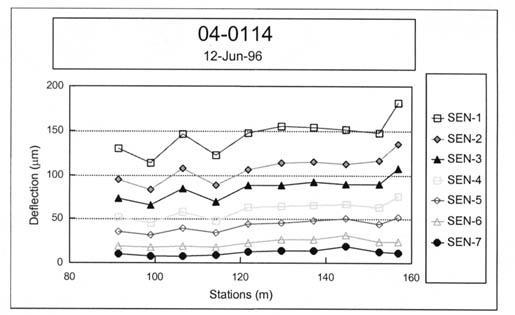
For the calculation of section average elastic properties, different maximum RMS error values were used to determine the average Young's modulus of a layer for a site and test date. Figures 13-16 graphically compare the average Young's modulus for different maximum RMS errors. The COV for the values shown in figures 13-16 varies from 5 to 15 percent along a test section. In general, a maximum RMS error of 2 to 3.5 percent had little to no effect on many of the test sections. In other cases, however, there were consistent and systematic changes in the average layer modulus with the maximum RMS error used to calculate the section average layer modulus.
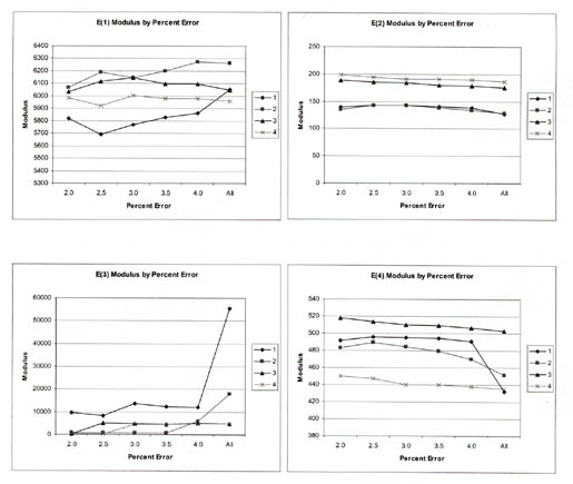
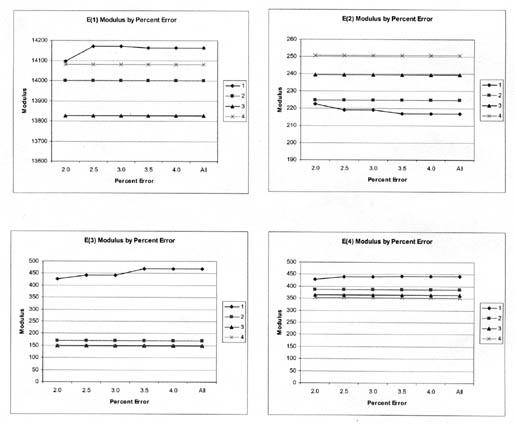
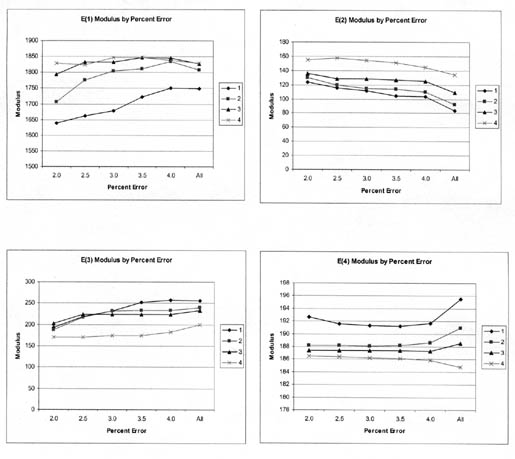

As expected, the maximum RMS error has a greater effect on the lower drop heights (smaller deflections) than on the higher drop heights (larger deflections). In general, the average elastic moduli calculated from all solutions with RMS error values of 3 percent or less are no different than those average values calculated with lower RMS error values.
In the third and fifth computed parameter tables, identified above (see table 6), all results were stored if a solution was obtained, even though some of the RMS errors for particular test points were greater than 4 percent. In the computed parameter summary tables (the fourth and sixth tables), only those solutions with RMS errors equal to or less than 2 percent were used in determining the average layer modulus and standard deviation along each test section on a specific test date. Selection of this maximum RMS error value of 2 percent is arbitrary and based on previous studies.
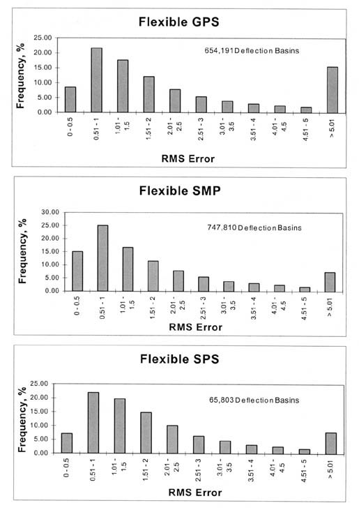
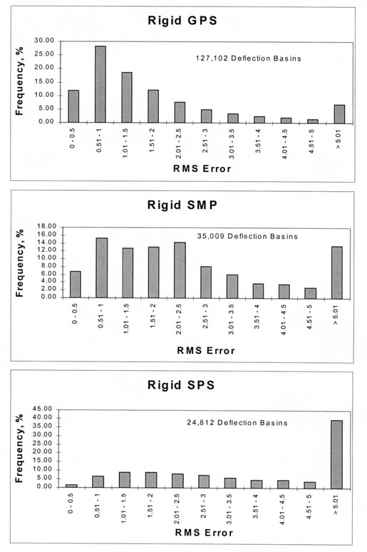
A total of 1,467,000+ deflection basins measured on the flexible pavement test sections were analyzed with MODCOMP4, and a total of 186,000+ basins measured on the rigid pavement test sections were analyzed. Figures 17 and 18 graphically illustrate the distribution of the RMS errors for the deflection basins measured on the flexible and rigid test sections that were analyzed with the linear elastic module of MODCOMP4, respectively. As shown, over 75 percent of the solutions have RMS errors less than 3 percent and are considered acceptable.
4.4 Brief Evaluation of Reasonableness of Solutions
A brief evaluation of the results was conducted to determine the reasonableness of the solutions. This review was focused mainly on the variation of the calculated moduli along the test section length, the change in the calculated moduli with season or month and with mid-depth temperature, and the effect of test load on the resulting moduli. This section of the report also presents examples of how these results can be used in pavement performance and/or material behavior studies.
4.4.1 Longitudinal Variation of Elastic Moduli. Figures 19-22 graphically illustrate examples of the longitudinal variation of the computed elastic moduli (Young's modulus) for selected test sections and different time periods. These results are typical of many other test sections. Some have extensive variability with both distance and time, whereas others are relatively uniform along the test section and with time.
These graphical comparisons are useful in judging whether the physical conditions of the pavement and subgrade soils may be significantly changing along the test section. In general, as the variability of the measured deflections increased, the variability of the calculated elastic layer moduli also increased and/or the number of reasonable solutions within a test section decreased.
For many test sections, a very stiff layer was computed for the subbase or stabilized subgrade layer of the pavement structure. These computed moduli are unrealistic and are not representative of the material, as shown in table 7 for test section 081053. These unrealistic moduli generally occurred for the more extreme Type II deflection basins (see figure 7). This condition was identified previously by Von Quintus and Killingsworth in a back-calculation study using the MODULUS software package.(3) Appendix C lists those test sections where the results for many of the test points are questionable.
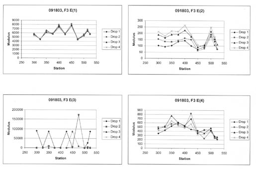
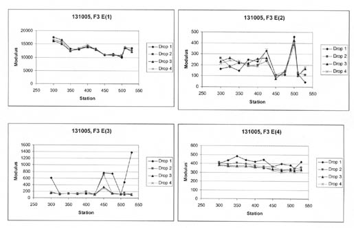
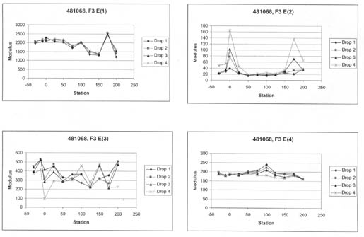
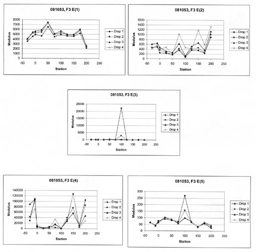
4.4.2 Wheelpath Versus Non-Wheelpath Measurements. At all of the LTPP test sections, deflections are measured both in the "outer wheelpath" (within the wheelpath) and in the "mid-lane" (between wheelpaths). The outer wheelpath measurements are identified as F3 in the database, whereas the mid-lane measurements are identified as F1. The back-calculation of layer moduli was completed for both sets separately.
Table 7 summarizes the average layer moduli computed for four test sections. For many of the test sections, there is no significant difference in the computed Young's modulus for the between-wheelpath and within-wheelpath measurement locations (e.g., test section 091803). However, significant differences were found for other test sections (e.g., test sections 081053 and 481068).
| LTPP Test Section |
Layer Designation |
Mid-Lane Mean, MPa |
Mid-Lane Standard Deviation, MPa |
Mid-Lane Coefficient of Variation, Percent |
Outer Wheelpath Mean, MPa |
Outer Wheelpath Standard Deviation, MPa |
Outer Wheelpath Coefficient of Variation, Percent |
|---|---|---|---|---|---|---|---|
| 081053 (March 1995) | 1 | 5,955 | 1,639 | 27.5 | 5,081 | 1,191 | 23.4 |
| 081053 (March 1995) | 2 | 1,355 | 528 | 38.9 | 641 | 370 | 57.8 |
| 081053 (March 1995) | 3 | 95 | 12 | 12.6 | 129 | 44.8 | 34.7 |
| 081053 (March 1995) | 4 | 127,086 | 107,095 | 84.3 | 32,559 | 38,370 | 117.5 |
| 091803 (August 1994) | 1 | 6,076 | 959 | 15.8 | 5,864 | 996 | 17.0 |
| 091803 (August 1994) | 2 | 190 | 60 | 31.6 | 189 | 54 | 28.6 |
| 091803 (August 1994) | 3 | 379 | 173 | 45.6 | 282 | 85 | 30.1 |
| 091803 (August 1994) | 4 | 450 | 110 | 24.4 | 421 | 128 | 30.4 |
| 131005 (January 1996) | 1 | 15,097 | 1,463 | 9.6 | 13,258 | 2,034 | 15.3 |
| 131005 (January 1996) | 2 | 291 | 130 | 44.7 | 216 | 98 | 45.4 |
| 131005 (January 1996) | 3 | 145 | 33 | 22.8 | 153 | 57 | 37.3 |
| 131005 (January 1996) | 4 | 368 | 26 | 7.1 | 342 | 27 | 7.9 |
| 481068 (August 1994) | 1 | 1,695 | 200 | 11.8 | 1,980 | 311 | 15.7 |
| 481068 (August 1994) | 2 | 216 | 104 | 48.1 | 57 | 51 | 89.5 |
| 481068 (August 1994) | 3 | 79 | 49 | 62.0 | 318 | 116 | 36.5 |
| 481068 (August 1994) | 4 | 193 | 5 | 2.6 | 179 | 8 | 4.5 |
Based on a brief review of the results, there is no consistent difference between the within-wheelpath and non-wheelpath measurements. For some of the test sections, however, low moduli were calculated for layers directly under the surface for within-wheelpath measurement locations. In most such cases, a higher modulus was calculated for the lowest layer, as shown in table 7 for test section 481068. These computations are believed to be unrealistic, even though the computations for both within- and between-wheelpaths were completed in the same within- and between-wheelpaths production run using the same pavement structure. Slight thickness variations, caused by plastic flow or lateral movement of the underlying materials close to the surface, may be a cause of this condition.
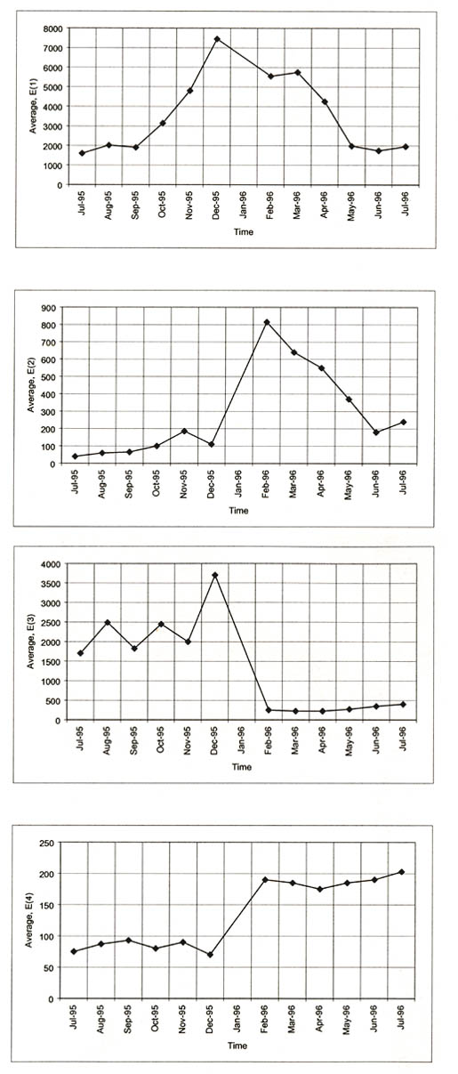
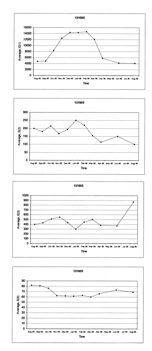
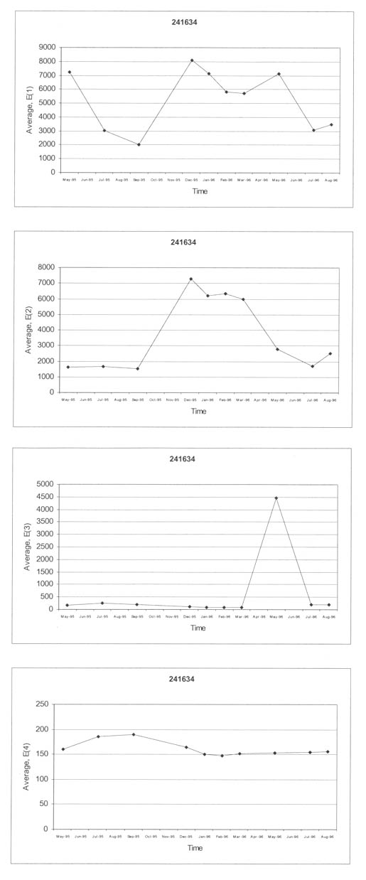
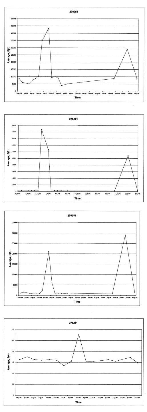
4.4.3 Seasonal or Monthly Effects. Figures 23-26 graphically illustrate examples of the monthly variation of the computed elastic moduli for the different layers of selected test sections. As shown, the moduli of the asphalt concrete layers increase for the winter months and decrease for the summer months. In addition, the modulus of the unbound aggregate layers and subgrade soils becomes extremely high during periods of possible freezing temperatures below the surface, as shown by the LTPP test section in Minnesota (276251).
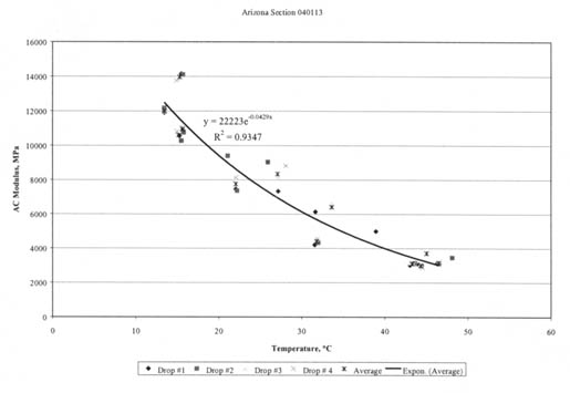
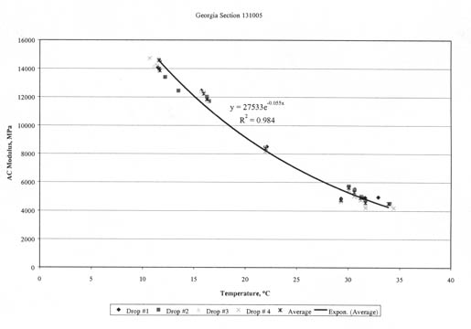
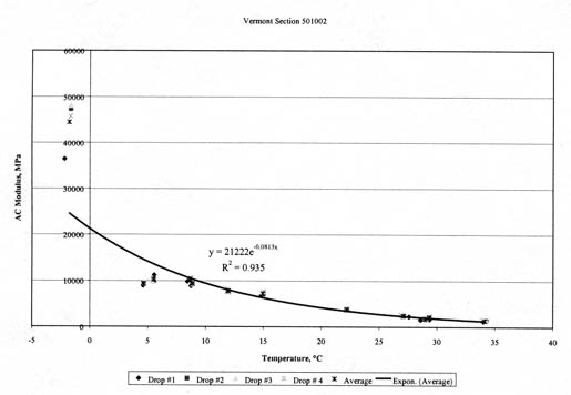
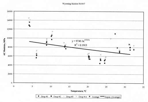
4.4.4 Temperature Effects. Figures 27-30 graphically illustrate examples of the computed elastic moduli for the asphalt concrete surface layer as a function of mid-depth temperature. As shown, the modulus of the asphalt concrete layer increases with decreasing temperatures. However, there are some cases where there are inconsistent changes in modulus with temperature. Some of these test sections were identified as having potential stripping in the HMA layer or were found to have extreme variations in the underlying support layers. Appendix C includes a summary of the overall average Young's modulus calculated at different temperature intervals for all HMA surface layers. As tabulated and expected, the average layer modulus decreases with increasing pavement temperature.
4.4.5 Time Effects. The SPS projects were used to look at systematic increases in the elastic moduli of the HMA and PCC surface layers as a result of hardening and curing. However, there are insufficient data to identify statistically any changes (increases) in the HMA and PCC moduli with time.
4.4.6 Stress Sensitivity from Linear Elastic Solutions. The linear elastic solutions were used to determine the change in computed elastic moduli (Young's moduli) with increasing load level. For fine-grained soils, the modulus decreased with increasing load level, as expected. For the coarse-grained soils, the opposite was the case, again an expected result, based on laboratory tests. These unbound materials or soils are stress-sensitive, and consistent changes were calculated with increasing load levels, as shown for some of the layers in figures 19-21.
The HMA layer is assumed to be a linear elastic material -- the modulus should not change with changes in load level. However, the computed elastic moduli resulting from the linear solutions were found to increase and decrease consistently with increasing load levels for many test sections (i.e., layer 1 in figure 22). Although these changes in moduli are not consistent with laboratory test results, they have been observed from other back-calculation studies using different programs. This observation could be just an artifact of the back-calculation process, the result of compensating errors or opposite changes in elastic modulus between two different but adjacent layers with increasing drop heights, and/or a stiffening or weakening effect with increased loads.
Again, the question becomes, "Is this a real condition or simply an anomaly from the back-calculation process?" It is believed that this condition may be more related to the interface condition between layers near the surface or damage that has occurred (accumulated) in the bound surface layers, rather than the true stress sensitivity of the layer.
4.5 Linear Versus Nonlinear Solutions
One of the primary purposes of this study was to compute the nonlinear elastic properties of the pavement materials and subgrade soils. In fact, the largest effort was devoted to calculating these nonlinear elastic properties. One of the questions to be answered at the beginning of the data study was whether the nonlinear solutions were worth the effort. Unfortunately, this question cannot be answered until a detailed comparison is completed between laboratory-derived properties and those computed from deflection basins.
Overall, fewer test points had acceptable RMS errors for the nonlinear solutions than for the linear elastic ones. Three possible explanations for this observation are listed below.
Another observation was that the HMA elastic moduli (bound layers) for the linear solutions were less than those for the nonlinear solutions but greater than the nonlinear solutions for the unbound layers. There are probably compensating differences between the bound or surface layers and unbound, subsurface layers. The cause for these differences is unknown but may be related to the interface condition of the surface layers/lifts, surface distortion, and/or microcracking of the HMA layers.
To begin to answer some of these questions would require a detailed analysis and comparison of the results with the laboratory tests and observations of the cores taken from the test sections, which was beyond the scope of work for this study.


 D
D