U.S. Department of Transportation
Federal Highway Administration
1200 New Jersey Avenue, SE
Washington, DC 20590
202-366-4000


Skip to content
Facebook iconYouTube iconTwitter iconFlickr iconLinkedInInstagram

Federal Highway Administration Research and Technology
Coordinating, Developing, and Delivering Highway Transportation Innovations

Report
This report is an archived publication and may contain dated technical, contact, and link information
Publication Number: FHWA-RD-03-041

Evaluation and Analysis of LTPP Pavement Layer Thickness Data

Statistical Formulations Used in the Skewness and Kurtosis Test

The following formulations for the combined skewness and kurtosis test were developed based on the reference [41].

For the skewness, we have:

Figure 76 in page 133 shows the skewness (k3) definition equation. k3 is equal to n divided by the product of n-1 and n-2 times the summation of the cubic difference between x sub i minus x bar, where n is the number of layer thickness measurements for the layer; x sub i is the individual thickness measurement along the section; x bar is the mean layer thickness.

Figure 76: Equation. Skewness definition.

For kurtosis, we have:

Figure 77 in page 133 shows the kurtosis (k4) definition equation. k4 is equal to 1 divided by the product of n-1, n-2, and n-3 times the difference between the product of n, n+1, and the summation of the fourth power of the difference between x sub i and x bar and the product of 3 and the square of the summation of the square difference between x sub i and x bar, where n is the number of layer thickness measurements for the layer; x sub i is the individual thickness measurement along the section; x bar is the mean layer thickness.

Figure 77: Equation. Kurtosis definition.

To evaluate the skewness and kurtosis tests results, the non-dimensional skewness and kurtosis coefficients are computed, as following:

Figure 78 in page 133 shows the skewness coefficient (g1) definition equation. g1 is equal to k3 divided by cubic s, where k3 is skewness and s is the standard deviation of the layer thickness data.

Figure 78: Equation. Non-dimensional skewness coefficient definition.


Figure 79 in page 134 shows the kurtosis coefficient (g2) definition equation. g2 is equal to k4 divided by the fourth power of s, where k4 is kurtosis and s is the standard deviation of the layer thickness data.

Figure 79: Equation. Non-dimensional kurtosis coefficient definition.

Based on the g1 and g2 values, the statistics and b2 are found next:

Figure 80 in page 134 shows statistic: the square root of b1 definition equation. Square root of b1 is equal to n-2 divided by the square root of the product of n and n-1 times g1, where n is the number of layer thickness measurements for the layer; g1 is the skewness coefficient.

Figure 80: Equation. Definition of statistic.


Figure 81 in page 134 shows statistic: the b2 definition equation. b2 is equal to the product of n-2 and n-3 divided by the product of n+1 and n-1 times g2 plus the product of 3 and n-1 divided by n+1, where n is the number of layer thickness measurements for the layer; g2 is the kurtosis coefficient.

Figure 81: Equation. Definition of b2 statistic.

To find z1 value, the following parameters are computed using and b2 statistics:

Figure 82 in page 134 shows the parameter A definition equation. A is equal to the product of the square root of b1 and the square root of the product of n+1 and n+3 divided by the product of 6 and n-2, where the square root of b1 is defined in Figure 80; n is the number of layer thickness measurements for the layer.

Figure 82: Equation. Definition of intermediate parameter A.


Figure 83 in page 134 shows the parameter B definition equation. B is equal to the quotient of the product of 3, square n plus 27 times n minus 70, n+1, and n+3 divided by the product of n-2, n+5, n+7, and n+9, where n is the number of layer thickness measurements for the layer.

Figure 83: Equation. Definition of intermediate parameter B.


Figure 84 in page 134 shows the parameter C definition equation. C is equal to the square root of the difference between the square root of the product of 2 and B-1 and 1, where n is the number of layer thickness measurements for the layer.

Figure 84: Equation. Definition of intermediate parameter C.


Figure 85 in page 135 shows the parameter D definition equation. D is equal to 1 divided by the square root of the natural logarithm of parameter C defined in Figure 84 in page 134.

Figure 85: Equation. Definition of intermediate parameter D.


Figure 86 in page 135 shows the parameter E definition equation. E is equal to the square root of the quotient of 2 and the difference between square C and 1, where parameter C is defined in Figure 84 in page 134.

Figure 86: Equation. Definition of intermediate parameter E.

The corresponding z1 value used as a skewness test statistic is the following:

Figure 87 in page 135 shows the skewness statistic z1 definition equation. z1 is equal to the product of parameter D and the natural logarithm of the total of parameter A divided by parameter E plus the square root of the total of the square of A divided E and 1, where parameter D defined in Figure 85 page 135; parameter A is defined in Figure 82 page 134; parameter E is defined in Figure 86 in page 135.

Figure 87: Equation. Definition of skewness test statistic z1.

To find z2 value, the following intermediate parameters are computed next:

Figure 88 in page 135 shows the mean of parameter b2 definition equation. meanb2 is equal to 3 times n-1 divided by n+1, where n is the number of layer thickness measurements for the layer.

Figure 88: Equation. Definition of the mean of intermediate parameter meanb2.


Figure 89 in page 135 shows the variance of parameter b2 definition equation. varb2 is equal to the quotient of 24 times n times n-2 times n-3 divided by the product of n+1, n+1, n+3, and n+5, where n is the number of layer thickness measurements for the layer

Figure 89: Equation. Definition of the variance of intermediate parameter varb2.


Figure 90 in page 135 shows the parameter F definition equation. F is equal to the quotient of the difference between b2 and meanb2 divided by the square root of varb2, where b2 is defined in Figure 81 in page 134; meanb2 is defined in Figure 88 in page 135; varb2 is defined in Figure 89 in page 135.

Figure 90: Equation. Definition of intermediate parameter F.


Figure 91 in page 135 shows the parameter G definition equation. G is equal to the product of the quotient of the product of 6 and n square minus 5n plus divided by the product of n+7 and n+9 and the square root of the quotient of the product of 6, n+3, and n+5 divided by the product of n, n-2, and n-3, where n is the number of layer thickness measurements for the layer.

Figure 91: Equation. Definition of intermediate parameter G.


Figure 92 in page 136 shows the parameter H definition equation. H is equal to 6 plus the product of 8 divided by G and the total of 2 divided by G plus the square root of the total of 1 and 4 divided by G square, where parameter G is defined in Figure 91 in page 135.

Figure 92: Equation. Definition of intermediate parameter H.

The corresponding z2 value used as a kurtosis test statistic is the following:
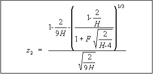
Figure 93 in page 136 shows the kurtosis statistic z2 definition equation. z2 is equal to the quotient of the total of 1 minus 2 divided by 9H minus the cubic root of the quotient of 1 - 2 over H divided by the total of 1 and F times the square root of 2 divided by H - 4 and the square root of the quotient of 2 divided by 9H, where H is defined in Figure 92 in page 136.

Figure 93: Equation. Definition of kurtosis test statistic z2.

The z1 and z2 statistics are used to obtain the p-values (the probability that values of the standard normal distribution are more extreme than the computed z1 and z2 statistics).

Federal Highway Administration | 1200 New Jersey Avenue, SE | Washington, DC 20590 | 202-366-4000
Turner-Fairbank Highway Research Center | 6300 Georgetown Pike | McLean, VA | 22101