Evaluation and Analysis of LTPP Pavement Layer Thickness Data

Procedures for the Kolmogorov-Smirnov Goodness-of-fit Test

The Kolmogorov-Smirnov test procedure involves the comparison between the experimental cumulative frequency and an assumed theoretical distribution function. If the discrepancy is large compared to what is normally expected from a given sample size, the theoretical model is rejected.

The Kolmogorov-Smirnov test procedure involves the following steps:

1. Sort layer thickness measurements in the ascending order.
2. Compute cumulative frequencies of each layer thickness observation S_n(x) using the following formula:

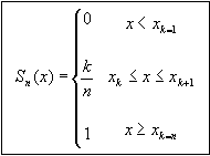
Figure 94: Equation. Cumulative frequencies definition.

Where x_k is a layer thickness value from sample of n layer thickness measurements sorted in the ascending order by thickness value. The k - index indicates the order of layer thickness observation in the sorted layer thickness array.

1. Select a candidate theoretical distribution function (for example, normal distribution).
2. Using the layer thickness measurements data, compute descriptive statistic values necessary for definition of the selected theoretical distribution (for example, mean and standard deviation).
3. Using selected theoretical distribution function and computed descriptive statistics, compute theoretical cumulative frequency values F(x_k) for each thickness value x_k.
4. Find the difference between the observed cumulative frequency value S_n(x_k) and the theoretically predicted cumulative frequency values F(x_k) for each x_k from the sample of n thickness measurements.
5. Select the maximum difference between the observed cumulative frequency value S_n(x_k) and the theoretically predicted cumulative frequency values F(x_k) called the observed maximum difference D_n or D-max statistic. This value is a measure of discrepancy between the theoretical model and the observed data.

Figure 95: Equation. D-max statistic definition.

8. Select level of significance α = 1 percent

9. Compute the critical value based on selected value of α. Based on value of n, is found as following

Figure 96: Equation. Critical value definition.

10. The Kolmogorov-Smirnov test determines whether, for specified level of significance α, the proposed distribution is an acceptable representation of the field data.

Figure 97: Equation. Kolmogorov-Smirnov test evaluation criteria.

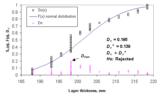
The following figure 98 demonstrates the results of the Kolmogorov-Smirnov test for a layer that did not pass the test of normality.

Figure 98: Chart. Example of Kolmogorov-Smirnov normal distribution goodness-of-fit test (DGAB layer SPS-1 LTPP section 01_0101).

Results of the Kolmogorov-Smirnov Goodness-of-fit Tests

The layer thickness measurements taken along the SPS LTPP sections for the structural layers were tested to determine how well the distribution of layer thickness measurements taken along the LTPP section follow selected theoretical distribution. The following table 69 provides the description of the layer and material types used in the SPS experiments. The table also provides information about layer thickness measurement sample sizes available in the LTPP database.

One data sample represents a group of measurements taken along the LTPP section for a specific layer and material type. There are 1,047 layers with thickness measurements along the LTPP section available in the LTPP database for the surface and base courses. The number of thickness measurements per layer and material type taken along the LTPP section ranges from 1 to 60. About 85 percent of all layers have at least 55 observations.

A total of 1034 pavement layers were tested to determine how well variability in layer thickness data along the LTPP section could be described using normal distribution. Kolmogorov-Smirnov goodness-of-fit test evaluated for level of significance alpha equal to 1 percent are summarized in table 70.

The results did not show as strong an indication of layer thickness distribution normality as the results of combined skewness and kurtosis test. This could be explained by lower power of Kolmogorov-Smirnov goodness-of-fit test compared to the combined skewness and kurtosis test. Low power indicates high probability of failing to reject the false null hypothesis.