Appendix B

Previous | Table of Contents | Next

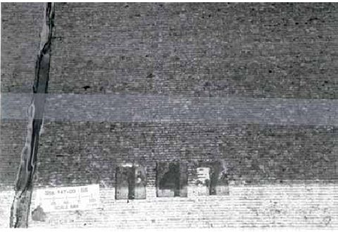
The test sections in Ohio were diamond ground between construction and the first monitoring visit (figure B1), so no evidence of surface scaling was visible. However, the diamond-ground surface did not experience any deterioration.

Figure B1. Typical surface textures after diamond grinding, Ohio test sections.

Nondestructive testing of the existing D-cracking susceptible concrete was conducted adjacent to the treated (or untreated) joints using Spectral Analysis of Surface Wave (SASW) methods. A schematic of the SASW test method is shown in figure B2. Actual testing at the Ohio test sections is shown in figure B3.

Figure B2. Schematic diagram of SASW testing (from Malhorta and Carino,Handbook on Nondestructive Testing on Concrete, CRC Press, New York, 1991.)

Figure B3. SASW testing at the Ohio test sections.

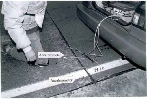
The method involved impacting the surface of concrete in such a way as to maximize the production of surface waves (R-waves) while minimizing the compression waves (P-waves). Two accelerometers mounted in line about 75 mm from the joint were used to measure the Rwave vibrations. Analysis of the phase shift of the vibrations between the two accelerometers was used to determine the R-wave velocity for various vibration frequencies. High-frequency vibrations are representative of shallow depths, while lower frequencies are more influenced by materials at greater depths in the pavement.

Figure B4 shows a typical R-wave velocity versus vibration frequency plot. The concrete pavement and subbase (base) portion are easily identified. The central section of the graph is dominated by noise resulting from waves reflected by the vertical edge of the pavement. This phenomenon is present in most of the R-wave velocity versus vibration frequency plots from the Ohio testing. Extensive analysis was conducted to filter out this reflection noise from the digital data obtained in Ohio.

Figure B4. Typical R-wave velocity versus vibration frequency plot.