U.S. Department of Transportation
Federal Highway Administration
1200 New Jersey Avenue, SE
Washington, DC 20590
202-366-4000
Federal Highway Administration Research and Technology
Coordinating, Developing, and Delivering Highway Transportation Innovations
 |
| This report is an archived publication and may contain dated technical, contact, and link information |
|
Publication Number: FHWA-RD-02-095 |
Previous | Table of Contents | Next
This chapter presents some case studies of the development, implementation, and evolution of QA specifications by the NJDOT. New Jersey was one of the first states to investigate and implement statistically based, QA specifications. As such, the NJDOT has a long history with QA specifications. These case studies have been selected primarily because the authors are very familiar with all of the steps involved and all of the specific details of the processes used in developing these specifications.
These case studies are intended to provide examples of how some QA specifications were initially developed and how they have evolved through the years. They are presented only to show the steps that are involved, the thought process that might be followed, and the types of decisions that must be made when developing QA specifications. They are NOT intended to represent the only, or even the best way, for any individual agency to develop its own QA specifications. These case studies have been selected for presentation because they clearly illustrate many aspects of the acceptance plan development process that are presented and discussed in the previous chapters and in the appendices.
As noted in the flowchart in figure 4, step 7.6, a decision that must be made very early in the specification development process is whether or not there is sufficient expertise within the agency, or if it will be necessary to seek outside assistance. This usually poses no problem as far as design, construction, inspection, and testing are concerned, because transportation agencies usually have many employees who are well trained in these areas. A critical area of expertise that often is not present, however, is statistical engineering.
Because this was recognized to be a vital prerequisite for a sound QA program, the NJDOT decided at the outset that it would be preferable to have the necessary statistical expertise as part of its in-house staff. Consequently, a new set of job specifications-the Statistical Engineer Series-was created to fill this perceived gap. Table 23 outlines the educational and experience requirements for the entry, intermediate, and supervisor levels; and the complete job specifications are contained in appendix N.
| Entry Level | Intermediate Level | Supervisor | |
|---|---|---|---|
| Engineering Degree | BSCE or equivalent | BSCE or equivalent | BSCE or equivalent |
| Applied Statistics Credits | 12 | 18 | 24 |
| Computer Science Credits | 6 | 6 | 6 |
| Experience, years | 2 | 3 | 4 |
The overriding philosophy of the NJDOT QA program is to use methods that are "simple but scientific," leading to the development of statistical construction specifications that
The first objective has been accomplished by using well-established statistical methods, and performing OC curve and EP curve analyses to verify that the acceptance procedures perform as intended. The second objective has been met by using pavement design methodology, engineering judgment, or a combination of both to develop prototype mathematical models to predict expected life from as-constructed quality levels. The third objective has been accomplished by choosing the simplest approaches possible and switching to more complex methods only if real data indicate the simple methods are inadequate in some way. The fourth objective has been achieved by recognizing both the technical and psychological benefits of positive-incentive provisions that reward excellent performers with bonuses in addition to the contract bid price. And, finally, the fifth objective has been accomplished by using life-cycle cost analysis methods to justify sufficiently severe payment reductions to strongly discourage poor quality workmanship.
A factor that must not be overlooked is that the construction industry is an indispensable partner in any highway agency's QA program. For any quality program to be successful for any extended period of time, it is essential that it be understood and supported by the contractors, producers, and suppliers who must work with it on a daily basis. This means that it must make sense to knowledgeable people in the field and must be perceived as fair and effective.
As this manual has previously emphasized, the surest way to guarantee that these conditions will be met is to include all the stakeholders in the specification development process. An approach that has worked extremely well for the NJDOT has been to form joint task forces that include representatives from the highway agency, FHWA, and the construction community. The specification and acceptance procedure should be well thought-out and thoroughly analyzed (OC curves, EP curves, etc.) before it is presented to the task force for their review since technical details are not easily worked out by group discussion. The agency can greatly enhance its credibility by being open to constructive criticism, and by providing valid, supportable answers to the many questions that will arise. By acknowledging that the specification is a prototype, and making the commitment to carefully monitor field performance and consider any necessary changes, the agency can expect to receive the support of the construction industry to proceed with a series of pilot projects. An additional condition that may be desirable for the field trials is to scale back the payment-adjustment provisions for the pilot projects, perhaps by as much as 50 percent. This allows both agency and contractor personnel to become more familiar and comfortable with the specification before it goes fully into effect.
The following are some of the basic principles of statistical specification writing, listed in the approximate chronological order of their discovery:
These principles, along with basic sampling and testing methodology, are applied in the case studies that follow.
Like most agencies, the NJDOT recognized that both the average level and the variability of construction work will affect expected performance. AAD and CI were not seriously considered as potential statistical quality measures, so this narrowed the range of possible choices to PD and PWL. Both are exactly equivalent from a mathematical standpoint, one being the complement of the other, but the NJDOT chose to use PD for specific reasons.
The primary reason was that it was the measure used in the original source documents. (23) A second reason was that the computation of total PD for a two-sided specification is slightly simpler and more intuitive than it is for PWL. And, finally, the use of PD casts the payment equation in a form that is easier to interpret by inspection, i.e., the constant term represents the maximum payment factor at PD = 0, and payment factors for increasing levels of PD gradually decrease from that maximum.
The PCC specification was the first of the modern statistical specifications developed by the NJDOT. What "modern" means is that most or all of the fundamental principles of statistical specification writing listed in the previous section are applied in a scientific manner. (The last three of this list were not felt to be necessary for the PCC specification but are included in case study 2.)
PCC acceptance is based on three quality characteristics-slump, air entrainment, and compressive strength. Since slump and air entrainment can be measured at the jobsite before the concrete is placed in the forms, the decision was made to use a pass/fail procedure for these measures. It was further decided that, if either slump or air entrainment (or both) were below the desired level based on the first set of tests, a single retempering would be permitted to attempt to bring the mix into the acceptable range. Typical acceptable ranges were ±25 mm for slump and ±1.5 percent for air entrainment, both of which represent ranges of about plus or minus two standard deviations.
Since compressive strength could only be evaluated after the concrete had cured, this characteristic was well-suited for acceptance by payment adjustment. Design strengths for four different classes of concrete are listed in table 24. The AQL was typically defined as PD = 10 percent below the class design strength (equivalent to PWL = 90).
It was the initial development of this specification in the late 1970s that led to a request to the Attorney General's office to furnish an opinion concerning the legality in the State of New Jersey of paying bonuses for superior quality. A review of existing statutes turned up nothing that specifically prohibited such an application so that, in the opinion of the Attorney General, such provisions were permissible. It was cautioned that it would be advisable to have evidence that extra quality, beyond what was specified in the contract documents, resulted in extra value to the State and the motoring public, thus justifying the use of bonus clauses. (This provided additional impetus to efforts already under way to establish quantified relationships that would ultimately be useful in developing performance-related specifications.)
Upon receipt of this opinion, it was decided to use a relatively modest bonus provision that provided a maximum payment of 102 percent for PCC items that tested out at the highest possible quality level of zero PD. Since the payment factors were applied to the in-place cost of the concrete, and concrete items tend to be relatively expensive, this provided substantial bonuses in many cases.
| Class | Class Design Strength | Typical Use | Pay Adj. Item | Tests per Lot1 | ||
|---|---|---|---|---|---|---|
| PSI | MPa | Initial | Retest2 | |||
| P 3 | 5500 | 37.9 | Prestressed members | Yes | 5 | 5 |
| A | 4200 | 29.0 | Bridge decks, columns, etc. | Yes | 5 | 5 |
| B 4 | 3700 | 25.5 | Pavement, footings, etc | If Yes: | 5 | 5 |
| If No: | 2 | 5 | ||||
| S | 2000 | 13.8 | Seal (tremie) | No | 1 | - |
1 A test is defined as the average strength of a pair of compression cylinders.
2 A retest, when required, is defined as the strength of an individual core.
3 Higher levels of Class P are frequently included by special provision.
4 Some Class B items may be declared as payment adjustment items.
More recently, the decision was made to increase both the positive incentives and the negative disincentives of the PCC payment schedule. NJDOT specification writers prefer to express payment schedules in terms of payment adjustment rather than payment factor and, accordingly, equations 29 and 30 were developed. As can be seen from equation 29, the AQL of 10 PD corresponds to a payment adjustment of zero (100 percent payment). The maximum bonus payment provided by equation 29 is +3.0 percent, while the minimum payment adjustment assigned by equation 30 is -50 percent.
where:
The payment schedule given by equations 29 and 30 illustrates a feature frequently used by the NJDOT, which has been well received by the construction industry. Provided that the quality level does not deviate too far from the desired level, the effect on the amount of payment adjustment is relatively moderate (equation 29). However, for seriously deficient quality, the level of payment falls off much more rapidly (equation 30).
Like many other agencies, the NJDOT also defines an RQL. This provision supersedes the payment equation and allows the agency the option to require removal and replacement whenever a poor quality level might severely impair the performance of an item. Based on the fatigue relationship of the AASHTO design equation, and consultations with pavement engineers, it is believed that a percent defective level of PD = 75 might result in a loss of service life of about 50 percent for New Jersey's PCC pavement design. (31) Based on this assumption, the RQL was set at PD = 75 with the provision that, if the agency elects not to enforce it, then the payment schedule given by equation 30 applies.
Ideally, it would be desirable to also have fatigue relationships for bridge decks and other structural items, similar to the AASHTO design equation for pavement, making it possible to predict the service lives of these items as a function of the as-constructed quality. An ongoing research study will attempt to determine if sufficient performance data are available to establish reliable relationships of this type. In the meantime, until such relationships can be developed, the NJDOT has decided to use the payment equations developed for pavement and apply them to all concrete items.
Unlike the application of payment adjustments, for which underestimates and overestimates of quality tend to balance out in the long run, there is no such compensating property associated with estimates of RQL material. In other words, it would not be considered an appropriate result if an agency falsely rejected a lot or two that were not actually as poor as RQL quality and, at the same time, mistakenly accepted a lot or two that truly were as poor as RQL quality. It is desired to keep the risk of either type of mistake at manageably low levels, and the easiest way to do this is to employ a retest to confirm the result when a seriously out-of-specification condition is detected. In the case of the NJDOT specification, a retest option occurs at the breakpoint of the payment schedule at PD = 50. Retest sampling rates are listed in table 24.
As noted in table 24, not all concrete items are accepted by payment adjustment. Some less critical items, usually Class B concrete, may be accepted by a pass/fail procedure. Provided that no individual strength test result falls below an appropriate limit, the item is accepted at full payment. Although it does not occur often, when a non-payment-adjustment item is rejected by the pass/fail procedure, it is then subject to retest and, from that point on, is treated as a payment-adjustment item.
The earlier version of this specification was implemented in the late 1970s, first on a series of pilot projects and, when that proved successful, it was included on all jobs thereafter. Initially, the construction industry was very apprehensive about the specification. Bid prices were somewhat higher than normal on the first few jobs, and some contractors hired testing laboratories to take companion cylinders to compare to the acceptance cylinders taken by the NJDOT. Also, it was obvious from the unusually high strengths obtained on the pilot projects (increase of about 7 Mpa) that contractors were being quite conservative with their mix designs.
As more experience was gained on the pilot projects, it was apparent that the independent testing labs were obtaining strengths that compared favorably with NJDOT results, and most contractors discontinued taking companion cylinders. Also, because of the conservative mix designs, strengths were higher than necessary and most contractors were earning bonuses. As time went on, the construction industry realized that with moderate care it could easily meet the requirements of the specification and bid prices tended to move back toward normal levels. Mix designs strengths tended to stay higher than in the past, but not as high as they were on the first few pilot projects.
When the latest version of the specification was implemented, the concern on the part of the construction industry was considerably less than it had been for the initial version. Still, it was deemed advisable to first implement the specification on a series of pilot projects. Once again, the experience was very favorable with the majority of lots earning full bonus, and the NJDOT plans to implement the specification on all future projects.
The development of the NJDOT Superpave specification consisted of three major phases. For the first phase in the early 1990s, the Superpave design method had not yet been developed. (24) At that time, the NJDOT was controlling the in-place density of its HMAC with an acceptance procedure based on the average air voids level determined from a series of cores taken from the completed mat. Although this specification had worked reasonably well for a number of years, it was noticed that the average often fell on the high side of the allowable range of 2.0-8.0 percent, and that individual values falling well above the upper limit of 8.0 percent were quite common. Consequently, it was decided to revise the specification and use a different quality measure, PD, designed to simultaneously control both the average level and the variability of the items to which it is applied.
Changing from an acceptance procedure based on the mean to one based on PD essentially redefined the AQL from a very lenient value of PD = 50 to a considerably more demanding level of PD = 10. Other modifications at the time included switching from a stepped to an equation-type payment schedule, adding a bonus provision for superior work, and including a remove-and-replace clause for seriously defective work.
A procedure and payment schedule, very similar to that described for the PCC specification in case study 1, were developed. Several pilot projects were constructed, quality levels were consistently good, and the specification was then broadly implemented.
In the late 1990s, a second phase of pilot projects introduced the change to the Superpave design method and, at the same time, the incorporation of a composite payment schedule based on three quality characteristics-in-place air voids, thickness, and smoothness. (25) Individual compound payment schedules were developed for each of these three characteristics, all based on PD as the statistical quality measure. Each of the payment schedules awarded bonuses for excellent quality, assessed moderate reductions for quality that strayed minimally from the desired level, and imposed more severe reductions for seriously deficient quality. Retest and remove-and-replace provisions were also included in this version of the specification. The composite payment equation combined the results of the individual payment equations, and the overall lot payment factor was taken as the average of the individual payment factors.
Several pilot projects were constructed with the phase two version of the specification. Although the quality ranged from good to excellent, with very few poor quality lots, it soon became apparent that certain features of the acceptance procedure were not optimal and should be improved. Thus began the third phase of the development of the Superpave specification.
A primary concern was that the method of averaging the payment factors for the individual quality characteristics did not accurately reflect the effect of the individual quality measures on pavement performance, thus falling short of relating the specification to performance. If the true performance model for HMAC pavement as a function of the three acceptance characteristics were known, it is believed that it would behave approximately as indicated in table 25.
| Quality Levels | Service Life |
|---|---|
| Poor in any one characteristic | Some loss |
| Poor in any two characteristics | Greater loss |
| Poor in all three characteristics | Substantial loss |
If the intuitive model in table 25 is even approximately correct, the method of averaging the individual payment factors in the prototype specification will not withhold sufficient payment to cover the likely costs of future repairs, nor will it pay an appropriate amount of bonus for truly superior quality. If the specification is to be truly related to performance, an additive process must determine the lot payment factor, although not necessarily a direct or fully additive process.
To confirm and approximately quantify the intuitive model in table 25, the NJDOT conducted a national survey to obtain estimates of pavement life for selected combinations of quality levels for the three measures-air voids, thickness, and smoothness. Responses were received from 35 States, of which four indicated that this information was not available, while another five failed a consistency check. This left a total of 26 responses, the averages of which are presented in table 26.
Table 26 provides the data from which it is possible to infer how experienced engineers believe various combinations of poor quality in the three characteristics affect pavement service life. The first row represents the reference condition, an expected life of 20 years when all quality measures are at their respective "good" levels. The next three rows include those cases for which just one of the three measures is at the "poor" level, producing an average expected life of (16.1 + 15.0 + 11.6) / 3 = 14.2 years. The next group of three rows includes those cases for which two of the three measures are at the "poor" level, producing a lower average expected life of (11.9 + 9.3 + 8.7)/3 = 10.0 years. The final row in table 26 represents the case for which all three measures are at the "poor" level, and produces a still lower expected life of 6.8 years.
| Initial Quality Levels | Expected Life (Years) | ||
|---|---|---|---|
| Smoothness | Air Voids | Thickness | |
| Good | Good | Good | 20.0 1 |
| Good | Good | Poor | 15.0 |
| Good | Poor | Good | 11.6 |
| Good | Poor | Poor | 8.7 |
| Poor | Good | Good | 16.1 |
| Poor | Good | Poor | 11.9 |
| Poor | Poor | Good | 9.3 |
| Poor | Poor | Poor | 6.8 |
1 Given as a reference point.
Since these results were consistent with the intuitive model in table 24, it was decided to proceed with the development of an additive model for this specification. Since it was planned to change to a new type of smoothness measure in the near future, it was decided to use only air voids and thickness in the composite payment schedule to be developed, and to treat smoothness separately.
At the time this specification was developed, the exponential model described in chapter 6 had not yet been developed, so the polynomial model for two characteristics given by equation 31 was used.
EXPLIF = C0+ C1 x PDVOIDS+ C2 x PDTHICK + C3 x PDVOIDS x PDTHICK(31)
where:
To determine the four unknown coefficients for this model, it is necessary to have four separate pieces of performance data, as shown in table 27. These values represent a consensus based on NJDOT field experience, plus an analysis using the AASHTO design procedure for flexible pavement using typical NJDOT data. (31)
| Thickness Quality | ||
|---|---|---|
| Air Voids Quality | PD = 10 | PD = 90 |
| PD = 10 | 20 yrs. | 10 yrs. |
| PD = 75 | 10 yrs. | 5 yrs. |
The four pieces of data in table 27 were then used to write four simultaneous equations that were solved to obtain the four unknown equation coefficients, producing the performance model given by equation 32.
EXPLIF = 22.9 - 0.163 PDVOIDS- 0.135 PDTHICK+ 0.000961 PDVOIDS x PDTHICK (32)
There are two ways that this model can be used to develop an acceptance procedure and adjusted payment equation. It can be used directly, first to estimate expected life, which is then substituted into a payment equation to determine the payment adjustment. Alternatively, it can be converted into a composite quality measure (see complete development in appendix K), in which case the payment adjustment is expressed as a function of the composite quality measure. For this specification, the NJDOT chose the latter approach, producing the expression for composite quality measure (PD*) given by equation 33:
PD* = 0.807 PDVOIDS+ 0.669 PDTHICK- 0.00476 PDVOIDS x PDTHICK(33)
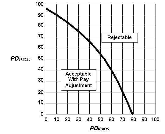
The use of the composite quality measure also provided an effective way to resolve another serious concern with the existing specification-the fact that the RQL provision was inconsistent in the way it dealt with simultaneous failures in two or more acceptance characteristics. The purpose of the RQL provision is to allow the agency the option to require removal and replacement, at the contractor's expense, of an item whose quality is so deficient that its performance may be severely impaired. Initially, the RQL for both air voids and thickness had been defined as PD > 75 so that if either air voids or thickness exhibited this level of quality the lot was considered rejectable. Later, based on attempts to relate quality to performance, it was decided that thickness PD could be as large as PD = 90 before such a severe consequence was justified. However, a more troubling problem was the inconsistency shown in table 28.
| Case | Quality Level | Rejectable? | |
|---|---|---|---|
| Air Voids | Thickness | ||
| 1 | PD = 10 (AQL) | PD = 90 (RQL) | Yes |
| 2 | PD = 75 (RQL) | PD = 10 (AQL) | Yes |
| 3 | PD = 74 (Almost RQL) | PD = 89 (Almost RQL) | No |
In cases 1 and 2, if either air voids or thickness is at the RQL while the other is at the AQL of PD = 10, this produces a reject condition. Case 3, in which both characteristics are almost at the RQL, clearly is far worse than the other two cases but does not lead to a reject condition.
Defining the RQL in a more appropriate way using the composite quality measure can rectify this inconsistency. Substituting either PDVOIDS= 10, PDTHICK= 90 or PDVOIDS= 75, PDTHICK= 10 into the composite quality measure equation produces PD* » 64, which, for practical purposes, is rounded to PD* > 65 as the RQL limit. Figure 43 illustrates how the RQL provision stated in this manner applies for all possible combinations of PDVOIDS and PDTHICK. It is the negative cross-product term that produces the concave downward shape, and any combination of PDVOIDS and PDTHICK falling on or above the line is considered rejectable. Note that the problematical case 3 in table 27 is clearly rejectable by this method and, also, that the curve passes through the two primary RQL points: PDVOIDS = 10, PDTHICK= 90 and PDVOIDS= 75, PDTHICK= 10. (The NJDOT has estimated that pavements falling anywhere on the RQL line in figure 43 have approximately a 50 percent loss of expected service life.)
The composite quality measure applies to both base and surface courses. In the NJDOT specification, total thickness is measured in conjunction with the surface layer. For base course, or for surface course of non-uniform thickness for which no thickness requirement applies, a default value of PDTHICK = 10 is used to compute the composite quality measure.
Because the expected service life of the pavement is approximately the same for any given value of PD*, this provides a convenient basis for a payment equation related to performance. Equations 34 and 35 are the equations for percent payment adjustment (PPA) developed by the NJDOT for air voids and thickness of mainline paving, ramps, and new shoulders in the latest Superpave specification. For existing shoulders, which experience has shown are more difficult to compact, the PPA computed with equation 34 or 35 is multiplied by a factor of 0.5. The lot payment adjustment is the PPA, expressed as a decimal, multiplied by the in-place dollar value of the lot. Alternatively, construction personnel sometimes use the PPAs to adjust the tonnage before totaling it up for payment, which produces the same result.
PD* < 40: PPA = 10 - 0.67PD* (34)
PD* > 40: PPA = 116 - 3.32 PD* (Minimum = -100) (35)
(RETEST: PD* > 40, REJECT: PD* > 65)
These payment equations incorporate the same feature described in case study 1. As long as the contractor can maintain reasonably good control so that PD* < 40, the consequences in terms of payment adjustment are relatively moderate. If, however, the process goes sufficiently out of control that values of PD* > 40 are obtained, the payment equation is much more steeply inclined and the consequences become more severe. Although it could be put at any point the agency considers appropriate, the NJDOT has found it convenient to put the retest option at the breakpoint of PD* = 40 in this compound payment equation.
Another drawback of the prototype specification was that, except for new construction, it did not include an incentive/disincentive provision for riding quality. In the near future, the NJDOT plans to switch to a profilometer-type smoothness measuring device, but, until that change is made, an interim incentive/disincentive plan has been developed for typical resurfacing projects that consist of milling followed by two paving layers. The plan is based on percent defective length (PDL), defined as the percent of the length of the pavement lot having deviations exceeding 3.175 mm in 3.048 m as measured with a rolling straightedge.
An agreement was reached with industry associations to use an incentive/disincentive plan that is less severe than is likely to be proposed when a new procedure is developed around a more sophisticated smoothness-measuring device. The interim payment schedule, based on the rolling straightedge, is given by equations 36 and 37. Pay adjustments (PA) for smoothness are calculated in units of $/m2, and the net payment adjustment for the lot is determined by multiplying by the lot area in square meters. As was done for air voids and thickness, the payment schedule consists of a compound payment equation that is moderate for quality that is reasonably under control, and more severe for quality that is clearly out of control. The payment adjustment computed for smoothness is added to any adjustment computed from the composite measure for air voids and thickness.
PDSMOOTH < 2.0: PA = 0.34 -
0.26 PDSMOOTH($/m2) (36)
PDSMOOTH >
2.0: PA = 0.72 - 0.45 PDSMOOTH($/m2)
(37)
(RETEST: PDSMOOTH > 2.0, REJECT: PDSMOOTH > 3.5)
There occasionally are resurfacing projects that do not meet the necessary criteria for thickness and smoothness to be accepted by payment adjustment. For these cases, table 29 illustrates how the new procedure applies across the full range of quality from the best (PDVOIDS = 0) to the worst (PDVOIDS = 100). Table 30 illustrates the performance over the same range when all three payment schedules apply.
| Base and Surface | Avg. PPA (%) | Lot Payment | ||
|---|---|---|---|---|
| PDVOIDS | PD* | $/m2 | $/Lane-Km | |
| 0.0 | 6.7 | +5.51 | +0.52 | +1,902 |
| 10.0 | 14.3 | +0.42 | +0.04 | +146 |
| 43.9 | 40.0 | -16.80 | -1.58 | -5,780 |
| 76.8 | 65.0 | -99.80 | -9.40 | -34,385 |
| 100.0 | 82.6 | -100.00 | -9.42 | -34,458 |
| Base Course | Surface Course | V & T PPA (%) | Total Lot Payment | |||||
|---|---|---|---|---|---|---|---|---|
| PDV | PD* | PDV | PDT | PD* | PDS | $/m2 | $/La-Km | |
| 0.0 | 6.7 | 0.0 | 0.0 | 0.0 | 0.5 | +7.76 | +0.94 | +3,439 |
| 10.0 | 14.3 | 10.0 | 10.0 | 14.3 | 0.5 | +0.42 | +0.25 | +914 |
| 43.9 | 40.0 | 0.0 | 59.8 | 40.0 | 0.5 | -16.80 | -1.37 | -5,011 |
| 43.9 | 40.0 | 30.0 | 30.0 | 40.0 | 2.0 | -16.80 | -1.76 | -6,438 |
| 43.9 | 40.0 | 49.6 | 0.0 | 40.0 | 3.5 | -16.80 | -2.44 | -8,926 |
| 76.8 | 65.0 | 0.0 | 97.2 | 65.0 | 0.5 | -99.80 | -9.19 | -33,617 |
| 76.8 | 65.0 | 53.2 | 53.2 | 65.0 | 2.0 | -99.80 | -9.58 | -35,044 |
| 76.8 | 65.0 | 80.6 | 0.0 | 65.0 | 3.5 | -99.80 | -10.26 | -37,531 |
| 100.0 | 82.6 | 100.0 | 100.0 | 100.0 | 3.5 | -100.00 | -10.28 | -37,604 |
Note: Costs based on 5.1 cm base, 5.1 cm surface, $38.59/Mg
V = Voids, T = Thickness, S = Smoothness, La-Km = Lane-Kilometer
Because table 30 includes all three measures of quality, both the incentives and the payment reductions cover a wider range than the corresponding values in table 29. In table 29, it is seen that excellent quality with zero PDVOIDS produces a PD* value of 6.7 and a bonus payment of $1902 per lane-kilometer. In table 30, this same level of quality combined with excellent quality in thickness produces a PD* value of zero, which, when combined with the excellent smoothness PD value of 0.5, corresponds to a bonus payment of $3439 per lane-kilometer. For extremely poor quality, both tables show that the maximum payment reduction is in the range of -$30,000 to -$40,000 per lane-kilometer.
The intermediate values in both tables present additional examples between these two extremes, and table 30 illustrates how different combinations of air voids and thickness PD can produce identical values of PD* (40.0 and 65.0), thus representing approximately equivalent performance from the standpoint of these two measures. It is this feature that makes the composite quality measure particularly well suited for relating performance to the payment schedules.
The procedure described thus far is practical and effective, but it contains a flaw that eventually should be addressed. Like the problem with the individual RQL provisions for air voids and thickness outlined in table 26 that was resolved by defining the composite quality measure, PD*, a similar inconsistency exists with PD* and PDSMOOTH. One way to resolve this problem would be to define a more complete composite quality measure that incorporates all three individual measures-air voids, thickness, and smoothness-and the general development of models for three or more quality characteristics is described in appendix L.
The NJDOT has chosen not to take this approach, however, because a major change in the current riding quality specification is imminent. When a new smoothness measuring device is selected, it is believed that it will be capable of being driven at or near traffic speed. In that case, it is likely that smoothness acceptance lots will no longer be treated in a piecemeal fashion along with air voids and thickness lots but, instead, may be defined as the entire project in one direction.
The new specification has payment schedules that are linked to expected performance, is easy to understand and apply, and provides increased incentive to provide good quality and avoid poor quality. To the extent possible it has been related to pavement performance through an analysis of expected service life and life-cycle costs. The ease of application can be seen in the outline in figure 44 that summarizes the key features of the complete acceptance procedure. With the use of the composite quality measure (PD*) and other refinements, the new specification requires a total of only five payment or payment-related equations to state the requirements for air voids, thickness, and smoothness. (The specification it replaced required more than a dozen payment equations to accomplish the same purpose.) And, finally, because the composite quality measure reflects the approximate additive nature of the effects of the three acceptance characteristics, both the incentives for excellent quality and the payment reductions for poor quality have been substantially increased, thus providing a strong incentive to produce good initial quality.
Another potential benefit of the increased incentive provision could foreshadow a profound change in the bidding process. Some NJDOT contractors have indicated that they have sufficient confidence in their QC operations and their ability to earn the incentive payments that this allows them to bid more competitively. If this continues to be the case, this may be an effective way for State agencies, which are legally bound by the competitive bidding system, to put more work in the hands of highly qualified contractors.
Base Course Air Voids and Surface Course Air Voids and Total ThicknessCompute Composite Quality Measure (PD*):
Compute Percent Payment Adjustment (PPA):
Surface Smoothness (Interim Procedure Until New Device Selected)Compute Payment Adjustment (PA, expressed in units of $/m2):
|
Figure 44. Outline of NJDOT Superpave Acceptance Procedure
This case study describes the development of a new acceptance procedure for HMAC pavement smoothness based on International Roughness Index (IRI) and illustrates some of the preparatory steps that must be taken, and assumptions that must be made, when performance models are not readily available.
As described in case study 2, an interim acceptance procedure for pavement smoothness had been developed as part of the latest version of the NJDOT Superpave specification. The interim procedure is based on measurements obtained with the rolling straightedge, a type of device the NJDOT has used for many years. By this method, smoothness was judged based on PDL, defined as the percent of the length of the pavement lot having deviations exceeding 3.175 mm in 3.048 m, computed from dye marks made on the pavement as the device is pushed at walking speed.
The rolling straightedge has the advantage of being relatively inexpensive and its operation is easily understood. From this standpoint it was well suited to use for acceptance by highway agencies, and also by contractors for QC purposes. However, it also has several drawbacks in that data collection is very slow and labor intensive, lanes being measured must be closed to traffic, and operators are exposed to fast moving traffic in adjacent lanes. More recently, questions about its accuracy and precision have been raised, and literature is available indicating that measurements made with a 3.048 m straightedge are incapable of being a good measure of pavement smoothness because they are insensitive to some of the longer wavelengths that are important in terms of vehicle dynamics, particularly in regard to trucks and larger vehicles that are known to be the major contributors to pavement damage. (26) Consequently, it was decided to switch to a new measure of smoothness, the IRI, a measurement that is computed directly from the longitudinal profile of the pavement and that is designed to be sensitive to vehicle dynamics.
An interim acceptance procedure for smoothness based on IRI has been developed and, for the initial phase-in period, it has been recommended that any lots subject to rejection or substantial payment reduction be retested with the rolling straightedge to make the final determination of acceptance. This will provide a grace period in which both the NJDOT and the construction industry can become familiar with the IRI as the new measure of smoothness. It is recognized that IRI and PDL do not correlate well because they measure different things, but it is believed that an interim procedure including the rolling straightedge will be more acceptable to both industry and NJDOT personnel.
Because the final decision will occasionally be based on the rolling straightedge during the phase-in period, there is the risk that pavements with poor IRI levels may be accepted, but that is exactly the situation now with acceptance based on PDL. There is also the likelihood that, on occasion, some pavements that are penalized based on IRI may appear to ride reasonably well in a passenger car and, if checked, may also have relatively low levels of PDL as measured with the rolling straightedge. This will most likely happen when the roughness consists of longer wavelengths that tend to affect larger and heavier vehicles, and it is a natural condition that must be expected to occur from time to time.
Since the NJDOT currently owns an ARAN that has recently been equipped with laser sensors to measure pavement profile, this vehicle will be used as the measurement device, at least initially. Several tests have been run to confirm that the measurements are sufficiently repeatable, and it was also discovered that the degree of repeatability can be improved by using a method that automatically triggers the collection of data at a specified starting point. Eventually, it will probably be necessary to purchase additional equipment dedicated solely to this function.
Since PD has been used as the statistical quality measure for other construction specifications, and it is desired to control both the mean level and the variability of IRI, the new specification will also be based on PD. Based on recent literature, (26) plus an analysis of IRI data obtained from New Jersey highways, it was determined that an appropriate upper limit for the prototype specification would be an IRI value of 1.26 m/km (or 80 inches/mile), combined with a typical value for the AQL of PD = 10. Since larger IRI values represent rougher pavement, this is a one-sided specification with a single upper limit, and the PD above this limit will be designated as PD80.
Unlike some statistical estimation procedures, for which the amount but not the location of the defective material is determined, the measurement of IRI produces a record of the pavement profile that makes it possible to identify the specific locations of rough areas. The availability of this information makes it possible to require corrective action, such as the selective grinding of particularly rough spots. Consequently, it was decided to define another quality measure, N100, which represents a count of the individual sections of pavement having an IRI of 100 inches/mile, or more.
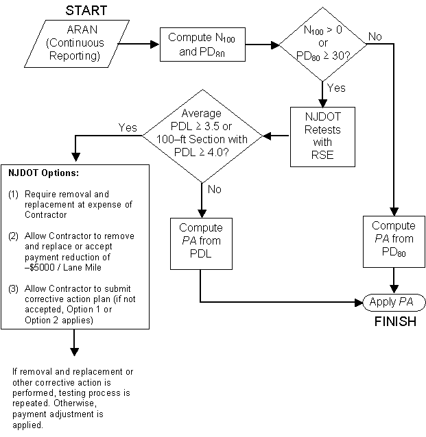
The acceptance procedure will be based on both quality measures-PD80 and N100. For the prototype specification, N100 will be used only as one of the triggers to determine when the rolling straightedge must be brought out to make the final determination of acceptance. Eventually, it may be used to determine when corrective action (selective grinding) will be required. A flow chart of the proposed procedure is shown in figure 45.
The need for the use of a bonus provision to assure fairness with acceptance procedures based on PD (or PWL) has been discussed earlier. What is less clear is whether such a clause is appropriate with an "identify and correct" type of acceptance procedure. However, because an extremely high level of smoothness would be expected to extend pavement life, and a high level of initial quality would also tend to expedite the construction process, it was decided that some degree of bonus was justifiable. It has also been observed that many other agencies have chosen to include bonus provisions as part of their smoothness acceptance procedures. The presence of a bonus provision will have the further advantage of promoting better cooperation from the construction industry, and it may also allow better contractors to bid more competitively.
In the past, the NJDOT has used specific starting and stopping stations to define smoothness lots, usually linked to time of construction (day's production, etc.). However, with the use of a measuring device that can be driven down the road at close to traffic speeds, it is recognized that it will be more practical to define acceptance lots as the entire project in one direction, or possibly a single lane for the entire project in one direction, rather than attempting to identify precise starting and stopping points for each day's production.
Similarly, it will be simpler (and is consistent with the LCC basis) if the payment adjustments are expressed in terms of dollars per lane-mile (or possibly dollars per square yard) rather than relating them to the bid price of the HMAC. (The interim acceptance procedure based on the rolling straightedge used with the latest Superpave pilot projects described in case study 2 expressed the payment adjustments in units of $/m2.)
However, to apply LCC to determine appropriate payment levels, it is necessary to have at least an approximate performance model to predict expected pavement life as a function of various levels of quality received. Since no such model based on IRI was readily available, it was necessary to rely on engineering knowledge and experience to develop a preliminary performance model.
As discussed in chapter 6, and developed further in appendix L, a particularly useful performance model is the exponential form given by equation 38,
EXPLIF = Ae-B(PD)C (38)
where
This model form is practical for several reasons. It tends to produce a sigmoidal ("S") shape (although this may not always occur) that is well-suited for many quality characteristics. This property recognizes that there is often a point of diminishing returns, both for extremely good quality and extremely poor quality. For example, performance tends to improve relatively rapidly for increasing quality within the region in which most quality estimates tend to fall but, for extremely high levels of quality, the additional improvement often is only marginal. The same effect is usually observed for extremely poor quality, primarily because expected life is limited at zero and, as quality continues to decrease, expected life approaches the horizontal axis asymptotically. Consequently, this model provides a measure of realism that is not always present with other model forms.
Another advantage of the exponential model given by equation 38 is that it only requires three "known" points to determine the unknown coefficients-A, B, and C. In most cases, it will be possible to identify three points that are sufficiently well known that the model can be specified reasonably accurately. Points that are typically used are the origin (at which PD = 0 and coefficient A is the maximum expected life), the AQL (at which the expected life equals the design life), and the RQL (at which expected life is dramatically reduced, but usually is not zero).
Very similar reasoning was used for the development of the IRI performance model. The primary determining point is the AQL at PD80 = 10, at which it is assumed that the typical service life of 10 years for a resurfacing will be achieved. Next, based on a consensus of experienced engineers, it was decided that the best possible quality level, represented by PD80 = 0, might extend the life of a typical resurfacing to about 12 years. Finally, instead of attempting to estimate the expected life at the RQL (which, at this point, is yet to be defined), it was decided to use the poorest possible quality level of PD80 = 100. Based on experience with very rough pavements, plus recent literature on IRI measurements, it was believed that such a pavement would not be immediately repaired in many cases and, consequently, would not have an expected life of zero.(26) However, this clearly is an extremely poor level of quality, and it was decided to assume an expected life of two years for purposes of developing the preliminary model. This produced the performance matrix given by table 31.
| PD80 | EXPLIF, in years |
|---|---|
| 0 | 12 |
| 10 | 10 |
| 100 | 2 |
The next step is to use the data from this performance matrix to determine the unknown model coefficients. By taking logarithms of both sides of equation 38, and substituting the values for PD80 and EXPLIF from table 31, it is possible to write three equations in three unknowns, and solve to obtain the performance model given by equation 39. (As a check, it is easy to demonstrate that, when the PD80 values from table 31 are entered, this equation returns the appropriate values for EXPLIF.)
EXPLIF = 12e -0.0186 ( PD80) 0.992 (39)
Once the performance model has been obtained, a method must be found to use the estimates of expected life it provides and convert them into appropriate levels of adjusted payment. To do this, the LCC equation derived in appendix I, which is repeated below as equation 40, can be used.
PAYADJ = C ( R D-R E ) / ( 1 - R O ) (40)
where:
The next step is to use equations 39 and 40 to develop table 32, relating PD80 to EXPLIF and PAYADJ. These results are then plotted in figure 46.
| PD80 | EXPLIF, in years (computed with equation 39) | PAYADJ, $ / Lane Mile (computed with equation 40) |
|---|---|---|
| 0 | 12.0 | +22,300 |
| 10 | 10.0 | 0 |
| 30 | 7.0 | -36,800 |
| 50 | 4.9 | -65,200 |
| 70 | 3.4 | -86,900 |
| 90 | 2.4 | -102,000 |
PAYADJ |
|
| ($1000/Lane Mile ÷ 1.61 = $1000/Lane Kilometer) |
Figure 46. Proposed Smoothness Acceptance Procedure Based on IRI
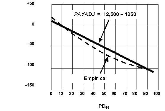
The empirical relationship obtained from equations 39 and 40 is plotted as a dashed line in figure 46. Since this relationship is nearly linear, it is approximated by the linear payment schedule that is given by equation 41, and plotted in figure 46. This represents the level of adjusted payment, in $ per lane-mile, that is justified by LCC analysis applied to the tentative performance model given by equation 39.
PAYADJ = 12,500 - 1250 PD80 (41)
An agency could choose to use any payment schedule that is less severe than this, as long as it provided sufficient incentive to produce the desired level of quality. For example, if management felt that the maximum bonus of +$12,500 per lane mile awarded by equation 41 was excessive, and wished to cap it at +$5000 per lane mile instead, then a somewhat shallower payment equation would be necessary. Since this shallower payment equation must go through the point PD80 = 10, PAYADJ = 0, in addition to the point PD80 = 0, PAYADJ = +$5000, its intercept is +$5000 and its slope is (5000 - 0) / (0 - 10) = -500, leading to equation 42 as just one of many alternate payment equations that might be used.
PAYADJ = 5000 - 500 PD80 (42)
For reasonably good levels of IRI quality, payment schedules such as equations 41 or 42 would apply. However, if either N100 > 0 or PD80 > 30 based on the initial tests, then a retest with the rolling straightedge is required, and the payment schedule given by equation 43, where PDL is percent defective length, applies (subject to the options listed on the flow chart in figure 45). Equation 43 is an interim payment schedule chosen to be very close to an existing schedule used with the rolling straightedge, and will no longer apply when the rolling straightedge is eventually phased out.)
PAYADJ = 3000 - 2308 PDL (43)
It can be seen by inspection that equation 43 pays a maximum bonus of PAYADJ = +$3000/lane mile at the best possible quality level of PDL = 0, and produces a payment adjustment of zero (100 percent payment) at the AQL of PDL = 1.3 for this measurement device. At the RQL value of PDL = 3.5, the payment reduction will be approximately -$5000/lane mile, provided the RQL provision in figure 45 is not enforced.
At the time of this writing, the final details of the specification are being worked out in preparation for testing on a series of pilot projects during the next construction season. As with other trial specifications, it is expected that the payment schedules will be reduced, perhaps by as much as 50 percent, for the initial pilot projects. Provided these projects are successful, it is planned to eventually exclude the use of the rolling straightedge before implementing the new specification widely on all projects.
Various modifications of this acceptance procedure are anticipated, both near-term and long-term. Depending upon the level of quality received, and on the ability of the construction industry to meet these requirements, some minor changes of the acceptance procedure may be appropriate in the near-term. Normally, the second phase would be to restore the full amount of the payment schedules, and then schedule additional pilot projects.
Long-term, the tendency will be to continue to "raise the bar" by specifying higher levels of quality as the construction industry gradually adapts to the new requirements and shows that they can consistently meet them. Also, since the performance model upon which the acceptance procedure is based is only tentative, it will be necessary to track performance so that, when some of the pavements constructed under this specification eventually require resurfacing, it will be possible to assess the adequacy of the model.