U.S. Department of Transportation
Federal Highway Administration
1200 New Jersey Avenue, SE
Washington, DC 20590
202-366-4000
Federal Highway Administration Research and Technology
Coordinating, Developing, and Delivering Highway Transportation Innovations
 |
| This report is an archived publication and may contain dated technical, contact, and link information |
|
Publication Number: FHWA-RD-02-095 |
Previous | Table of Contents | Next
Statistical construction specifications use characteristics measured at the jobsite to make appropriate acceptance decisions. The decision might be to pay a small incentive for unusually high quality, pay the contract price for an item that meets the specified quality level, accept the item at reduced payment when the quality is marginally deficient, or require removal and replacement if the quality is seriously defective. It may also be necessary to make an intermediate decision concerning whether or not additional tests should be performed to check marginal results, or to confirm that the quality is sufficiently poor that removal and replacement is warranted.
There are, therefore, several different types of decisions to be made and, when there are also different types of tests to be performed on a particular construction item, it can become a complex matter to design an acceptance procedure that is fair, effective, and free from inconsistencies. As an example of one type of inconsistency that can occur, consider the performance of a rejection provision for air voids and thickness of HMAC pavement as outlined in table 50.
Case |
Quality Level |
Rejectable? | |
|---|---|---|---|
Air Voids |
Thickness | ||
1 |
PD = 10 (AQL) |
PD = 75 (RQL) |
Yes |
2 |
PD = 75 (RQL) |
PD = 10 (AQL) |
Yes |
3 |
PD = 74 (Almost RQL) |
PD = 74 (Almost RQL) |
No |
The RQL for both air voids and thickness has been defined as PD > 75. In other words, if either characteristic exhibits this level of quality, the lot may be declared rejectable. However, as seen in table 50, case 3 is clearly the worst case, yet it does not trigger the RQL provision whereas the other two cases do.
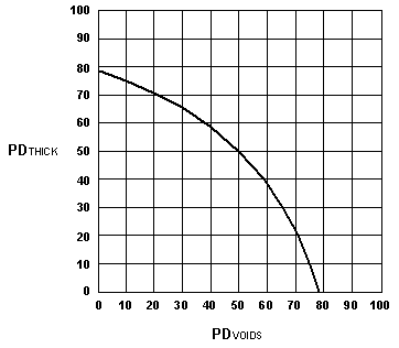
To correct this inconsistency, a composite RQL provision can be derived as a joint function of the two quality measures. Equation 95 and figure 64 illustrate an RQL provision of this type derived from basic performance considerations (see appendix J).
| 1.273 PDVOIDS + 1.273 PDTHICK - 0.0109 (PDVOIDS x PDTHICK)>100 | (95) |
 |
Figure 64. Graph of RQL Provision Given by Equation 95 |
All points on the curve in figure 64 are judged to be equally detrimental in terms of pavement performance, and any combination of PDVOIDS and PDTHICK falling on or above the curve would be judged to be rejectable. Although equation 95 was developed specifically to make an appropriate rejection decision based on the joint quality measures of air voids and thickness, it suggests how a general family of curves might be developed that would be useful for the retest and payment adjustment decisions that must also be made.
To illustrate how this can be done, equation 96 presents a general performance model in which EXPLIF represents the expected life of the pavement in years, the C terms are coefficients to be determined, and PDVOIDS and PDTHICK are the measures of air-voids and thickness quality. To determine the four unknown coefficients in equation 96, four known points spanning a wide range of quality are needed. These may be obtained from any valid source-agency experience, established performance models, or field experiments-and the values presented in table 51 were obtained from a combination of these sources (see appendix J).
EXPLIF = C0 + C1 (PDVOIDS) + C2 (PDTHICK) + C3 (PDVOIDS x PDTHICK) |
(96) |
| PDTHICK = 10 |
PDTHICK = 90 |
|
|---|---|---|
|
PDVOIDS = 10 | 20 years | 10 years |
|
PDVOIDS = 75 | 10 years | 5 years |
Substituting the values from table 51 into equation 96 produces four equations in four unknowns given by equations 97 through 100:
C0 + 10 C1 + 10 C2 + 100 C3 = 20 |
(97) |
C0 + 75 C1 + 10 C2 + 750 C3 = 10 |
(98) |
C0 + 10 C1 + 90 C2 + 900 C3 = 10 |
(99) |
C0 + 75 C1 + 90 C2 + 6750 C3 = 5 |
(100) |
The solution for this set of simultaneous equations provides the coefficients to be substituted into equation 96 to obtain the performance model given by equation 101:
EXPLIF = 22.9 - 0.163 PDVOIDS - 0.135 PDTHICK + 0.000961 (PDVOIDS x PDTHICK) |
(101) |
This equation predicts that excellent quality (PDVOIDS = PDTHICK = 0) will extend pavement life beyond its design life of 20 years to almost 23 years. At the other extreme, the worst possible quality level in terms of percent defective (PDVOIDS = PDTHICK = 100) produces an expected life of just less than three years. As a further check of the derivation of equation 101, the four combinations of quality levels listed in table 51 can be entered into this equation to demonstrate that it returns the table 51 values for expected life. The complete family of performance curves is plotted in figure 65.
Because equation 101 provides a direct estimate of expected life as a function of the individual quality measures, it can form the basis for a performance-related payment schedule, as demonstrated in chapter 6. Alternatively, equation 101 can be used to develop a single, composite quality measure that will simplify the overall acceptance process and the various decisions to be made.
Since the quality measure used for this example is percent defective (PD), which ranges from a minimum of zero to a maximum of 100, it will be convenient to develop a composite quality measure (PD*) that spans that same range. As derived, the value of EXPLIF in equation 101 ranges from 2.71 to 22.9. To map equation 101 onto the desired response surface, the following three operations must be performed on the terms on the right-hand side of the equation:
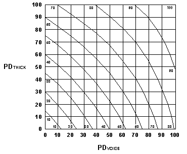
This produces equation 102, which can be demonstrated to produce values of PD* ranging from zero to 100 as the individual quality measures cover the entire range from PDVOIDS = 0, PDTHICK = 0 to PDVOIDS = 100, PDTHICK = 100. To provide a better understanding of how this equation performs, a family of curves is plotted in figure 66.
PD* = 0.807 PDVOIDS + 0.669 PDTHICK - 0.00476 (PDVOIDS x PDTHICK) |
(102) |
To demonstrate the practicality of the composite quality measure, a complete acceptance procedure must be specified. This includes the AQL, the RQL, any retest provision, and the payment schedule.
For illustration purposes, suppose the agency has decided that the AQL, the quality level at which the pavement is to be accepted with no price adjustment, is defined as PDVOIDS = PDTHICK = 10. Suppose, also, that if the combined effects of poor quality in air voids and thickness are such that the performance relationship of equation 101 (shown graphically in figure 65) indicates an expected life of 10 years, or less, the pavement is considered to be rejectable and the agency reserves the option to require removal and replacement. Also, since agencies might want to specify some intermediate level of quality at which the agency has the option to require additional tests before accepting what might turn out to be seriously defective work, it will be assumed for this example that the retest option is in effect whenever the performance model of equation 101 indicates an expected life of 15 years or less. And finally, based on a life-cycle cost analysis of the cost of premature pavement failure, (32) the projected net present cost to the highway agency of a 20-year design pavement failing after only 10 years is estimated to be approximately $50,000 / lane-kilometer.

Figure 66. Graph of Composite Quality Measure (PD*) Given by Equation 102
With this information, the complete acceptance procedure can be specified. To determine the comparable value of PD* associated with the AQL, the values of PDVOIDS = PDTHICK = 10 are substituted into equation 102 to obtain PD* = 14 as the AQL. Therefore, the payment equation must produce a payment adjustment of zero at PD* = 14. To determine the value of PD* associated with the RQL, any combination of values on the 10-year-lifeline in figure 65 can be substituted into equation 102. For example, entering PDVOIDS = 60 and PDTHICK = 40 into equation 102 produces PD* > 64 as the RQL. Similarly, any combination of values on the 15-year-lifeline, such as PDVOIDS = 20 and PDTHICK = 40, produces PD* > 39 as the retest provision. Finally, assuming a simple linear payment equation will be sufficient, the payment schedule given by equation 103 is derived.
|
PAYADJ = 14,000 - 1000 PD* |
(103) |
Where: PAYADJ = lot payment adjustment ($ / lane-kilometer), and
PD* = composite quality measure.
It can be seen that when PD* is at the AQL value of 14, equation 103 produces a payment adjustment of zero, as desired. Similarly, when PD* equals the RQL value of 64, the desired payment reduction of -$50,000 / lane-kilometer is obtained. For truly excellent quality, where PDVOIDS and PDTHICK are both zero, PD* also equals zero and the payment equation awards a maximum bonus of $14,000 / lane-kilometer. At the other extreme, when PDVOIDS and PDTHICK both equal 100, PD* also equals 100 and the payment equation assigns the maximum payment reduction of -$86,000 / lane-kilometer. In between, all payment adjustments are related to performance in that all quality levels that fall on any particular pavement-lifeline in figure 65 will receive the same level of payment. Note also that both the retest provision and the RQL provision, because they are stated in terms of the composite quality measure, avoid the inconsistency illustrated in table 50.
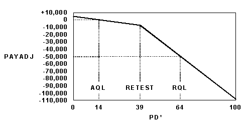
The maximum incentive of $14,000 / lane-kilometer paid by equation 103 is the result of choosing to make the payment equation linear. If the agency were not comfortable with this large an incentive, perhaps because there were other factors that might prevent the pavement from fully benefiting from superior quality in the measured quality characteristics, then it may be appropriate to use a compound payment equation that is less steeply inclined in the region of the AQL. For example, suppose the agency determined that the maximum incentive to be paid under any circumstances was $5000 / lane-kilometer, but that the payment reduction of -$50,000 / lane-kilometer at PD* = 64 was still considered to be justified. Since it is necessary to produce a payment adjustment of zero at the AQL of PD* = 14, two separate payment equations will be required, resulting in a compound payment equation. Although the breakpoint of the compound equation can be at any desired point, it will be convenient to put it at the retest level of PD* = 39. The resulting payment schedule is given by equations 104 and 105, and is illustrated in figure 67.
PD* < 39: PAYADJ = 5,000 - 357 PD* |
(104) |
Extension to Three Variables
Although it is possible to apply this same process when there are three individual quality characteristics, more data are required and it will be necessary to solve eight simultaneous equations to account for all the cross‑product terms. Therefore, when there are three or more variables, it is recommended that the exponential model, which is described in chapter 6 and appendix L, be used.
 |
| Figure 67. Compound Payment Schedule Given by Equations 104 and 105 |
Not all individual quality measures are equally suitable for incorporation into a composite measure. Measures that are best suited are those that jointly affect performance in such a way that, within practical limits, higher quality in one tends to offset deficiencies in the others. Another requirement is that they be convenient to measure in association with each acceptance lot. The example involving air voids and thickness of HMAC pavement is obviously well suited, as would be strength and thickness of PCC pavement.
Measures that are less suitable are those that are dominant or controlling, or which are less convenient to measure on individual lots. For example, an agency might choose to use a stand-alone acceptance procedure for pavement smoothness if it were felt that riding quality should be evaluated on its own merits without regard to the other quality measures, or if it were considered more convenient to evaluate riding quality on large sections of the project at a single time rather than on a lot-by-lot basis.
An alternate method to develop performance-related payment equations for multiple quality characteristics is to first develop a composite quality measure that is a function of the individual quality measures. An example was presented in which performance relationships for air voids and thickness of HMAC pavement were used to develop a single quality indicator, PD*, as a function of the individual quality measures, PDVOIDS and PDTHICK.
The methodology offers both mathematical simplicity and a sound empirical basis in that it can be developed from performance data obtained by a variety of means. It is generally applicable in any situation involving multiple acceptance criteria for which performance results are known or can be modeled or approximated. It is well suited for use with PD or PWL, but is not necessarily limited to those quality measures. It avoids certain inconsistencies in practice that may occur with other methods for dealing with multiple quality characteristics, and it leads to rational payment schedules in that it assures that all combinations of individual quality measures that predict the same level of expected life will receive the same amount of payment adjustment.
The use of a composite quality measure provides a practical and effective means to make three different types of acceptance decision-retest, reject, and payment adjustment-all keyed to a common performance model. But in spite of these many advantages, perhaps its strongest selling point is the ease with which it can be understood and applied, as demonstrated by the following procedural steps for the HMAC example: