U.S. Department of Transportation
Federal Highway Administration
1200 New Jersey Avenue, SE
Washington, DC 20590
202-366-4000
Federal Highway Administration Research and Technology
Coordinating, Developing, and Delivering Highway Transportation Innovations
 |
| This report is an archived publication and may contain dated technical, contact, and link information |
|
Publication Number: FHWA-RD-02-095 |
Previous | Table of Contents | Next
This appendix includes a brief explanation and discussion of the OCPLOT computer simulation program for developing OC and EP curves. This program was developed as part of FHWA Demonstration Project 89, and a much more thorough discussion of the OCPLOT program is provided in the manual for that project. (18)
In the case of pass/fail acceptance procedures, OC curves can be computed directly or constructed with the aid of specialized mathematical tables. For acceptance procedures with adjusted payment schedules, the construction of EP curves usually requires computer assistance. Program OCPLOT uses computer simulation to develop both OC and EP curves.
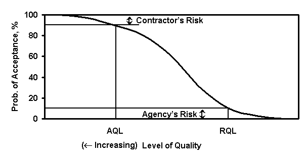
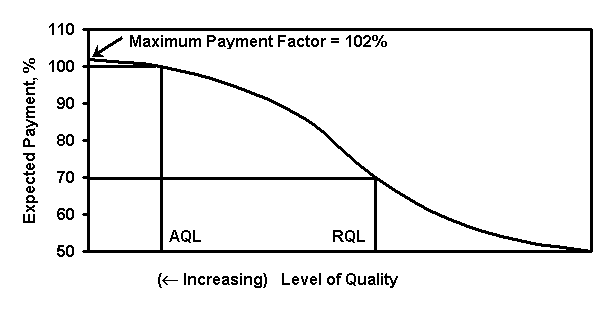
Program OCPLOT is designed to analyze the types of acceptance procedures typically used in the highway field. This includes pass/fail procedures, leading to the type of OC curve shown in figure M1, and payment adjustment procedures, leading to the type of EP curve shown in figure M2.
Figure M3 lists some of the options that may be selected from the primary menu. The various items appear on the screen one at a time in a logical sequence, and later items are dependent upon the responses to earlier ones. The versatility of the program is apparent from the many different ways these selections might be combined.
When the selections from the first menu are complete, the menu will appear similar to that shown in figure M4. The prompt "Press any key to continue" at the bottom of the display provides a pause that gives the user the opportunity to use the <ESC> key to go back and change some values or press the <PrintScreen> key to save the screen to a file if a record of the menu selections is desired. Striking almost any other key will cause the second menu in figure M4 to appear.
|
Figure M1. Conventional OC Curve for Pass/Fail Acceptance Procedure |
|
Figure M2. Typical EP Curve for Acceptance Procedure with |
| ACCEPTANCE METHOD | |
| Pass/Fail | TYPE OF PLAN |
| Pay Adjustment | Attributes Variables |
| QUALITY MEASURE | |
| Percent Defective (PD) | |
| Percent Within Limits (PWL) | |
| LIMIT TYPE | |
| SingleSided | |
| Double Sided | |
| PAY EQUATION TYPE | |
| Linear/Nonlinear | Enter Values |
| MAXIMUM PAY FACTOR | |
| Yes | Enter Values |
| No | |
| ACCEPTABLE QUALITY LEVEL (AQL) | |
| Enter Value | |
| REJECTABLE QUALITY LEVEL (RQL) | |
| Enter Value | |
| RQL PROVISION | |
| Yes | Enter RQL Payment Factor |
| No | |
| RETEST PROVISION | |
| Yes | INITIAL TESTS |
| No | Combined Discarded |
| SAMPLE SIZE | |
| Enter Value(s) | |
Figure M3. Selections Available in Program OCPLOT |
|
| ENTER THE FOLLOWING INFORMATION |
|
| ACCEPTANCE METHOD |
ACCEPTABLE QUALITY LEVEL PD = 10 |
| QUALITY MEASURE Percent Defective |
REJECTABLE QUALITY LEVEL PD = 50 |
| LIMIT TYPE Double-Sided |
RQL PAY FACTOR PF = 70 |
| PAY EQUATION PF = 102 - .2 PD |
RETEST PROVISION None |
| MAXIMUM PAY FACTOR PF = 102.0 |
SAMPLE SIZE 10 |
Press
any key to continue |
|
| <ESC> = Back |
<END> = Exit |
Second Menu:
|
SELECT LEVEL OF PRECISION |
|
(1) Low Faster Execution (2) Intermediate (3) High Slower Execution SELECTION |
|
<ESC> = Back <END> = Exit |
Figure M4. First and Second Menus for Program OCPLOT |
Because program OCPLOT uses computer simulation to analyze whatever acceptance procedure has been specified, it is very computationally intensive and the execution speed is dependent upon the level of precision selected from the second menu. Table M1 lists the number of replications performed for the different levels of precision.
|
Precision Level |
Number of Replications |
|---|---|
|
1 |
200 |
|
2 |
1,000 |
|
3 |
5,000 |
Selection 1 provides the fastest execution, which is useful for exploratory work but may not be good enough to report as a final result. When this level is selected, 200 sample sets of the desired size are randomly generated from a normal population for each of several known levels of quality.
Each sample set is evaluated in accordance with the acceptance plan specified in the primary menu and the results are stored in memory for subsequent analysis. This is far more thorough and many times faster than testing the acceptance procedure with a field trial. (A field trial would be appropriate only if the procedure survives this initial check.)
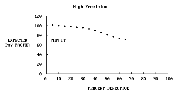
Selection 2 from the second menu provides an intermediate level of precision for which 1000 sample sets are generated at each quality level. This level of precision is usually satisfactory to report as a final result, producing points for the OC curve, representing probability of acceptance, or the EP curve, representing the expected payment factor, that are typically accurate to within one or two units. If still better precision is desired, selection 3 will cause 5000 sample sets to be generated at each quality level. This level of precision tends to produce a smooth line when the OC or EP curve is plotted.
Once the precision level is selected from the second menu, the computational process begins. For either low or intermediate precision, program OCPLOT displays detailed information at the two key points at which risk levels are usually expressedthe AQL and the RQLas shown in figures M5 and M6. This serves two important purposes. For users less familiar with statistical estimation procedures and acceptance plans, the graphical displays at the AQL and RQL are both informative and educational. It may come as a surprise to some, for example, how widely distributed the quality estimates are, especially for small sample sizes. For users more familiar with statistical acceptance procedures, these displays provide assurance that the simulation process is working properly. The actual displays on a color monitor are colorcoded to clearly distinguish acceptable and rejectable results and the corresponding payment factors.
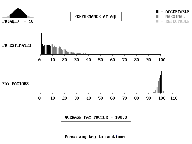
Figure M5. Typical Display at AQL at Intermediate Precision by
Program OCPLOT
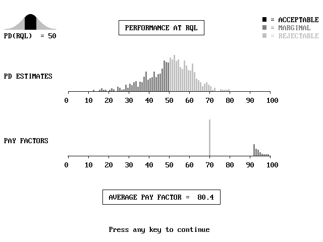
Figure M6. Typical Display at RQL at Intermediate Precision by Program OCPLOT
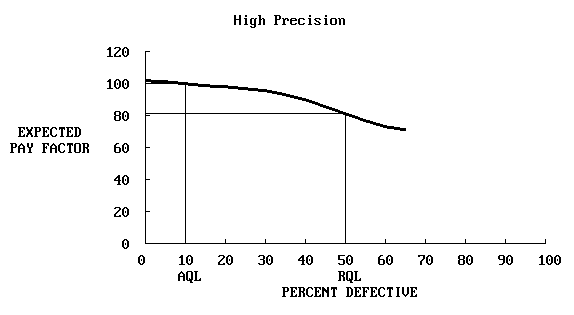
Although the AQL and the RQL are probably the most important points at which it is desirable to know how the acceptance procedure will perform, it usually is useful to have a plot of the entire OC or EP curve that provides a picture of the performance over the complete range of quality that might be encountered. The prompt at the bottom of the screen instructs the user to strike any key to continue with this step to obtain the display shown in figure M7. The horizontal and vertical axes and the two previously calculated points at the AQL and the RQL appear on the screen immediately. The remaining points appear one at a time at a speed determined by the level of precision that has been selected and the speed of the machine running the program.
After all the points have been calculated and plotted, the user may strike any key to connect the points with a solid line. Following this, the next key stroke will add vertical and horizontal lines highlighting the performance of the acceptance plan at the AQL and RQL, as shown in figure M8. And, like the histograms in figures M5 and M6, any of these displays may be saved to a file by using the <PrintScreen> key.
Following this display, striking a key will produce the menu shown in figure M9. If the first item in this menu is selected, the output shown in figure M10 is displayed. This permits the user to save the values of the data points shown in figure M7 from which the OC curve was constructed. The other selections in this menu make it possible to return to earlier points in the input stage of the program or to exit the program.
Example M1: Pass/Fail Attributes Procedure
Attributes acceptance procedures are based on measures that are counted rather than computed, such as the number of defects on an item of production or the number of test results falling outside specification limits. In contrast, variables acceptance procedures are based on statistical parameters that are computed, such as the mean and standard deviation, and lead to the estimation of PD or PWL.
Advantages of attributes procedures are that they are simple to apply and they require no assumptions about the underlying distributional form of the population being sampled. For example, a typical attributes procedure might require that a sample of size N = l0 be taken and that no more than C = 2 test results may be outside the specification limits, where "C" is referred to as the acceptance number. A disadvantage is that they require larger sample sizes to achieve the equivalent discriminating power of a variables procedure. Variables procedures, because of their inherently greater efficiency, are generally preferred whenever the requirement for a normallydistributed population is reasonably satisfied.
|
| FigureM7. Points on EP Curve Plotted by Program OCPLOT |
 |
| Figure M8. Display of EP Curve Plotted by Program OCPLOT with AQL and RQL Performance Highlighted |
|
SELECT DESIRED OPTION |
|
(1) Display operating characteristic table (2) Select precision level and run again (3) Change some values and run again (4) Run again with new input data (5) Exit program SELECTION |
| <ESC> = Back <END> = Exit |
Figure M9. Third Menu for Program OCPLOT
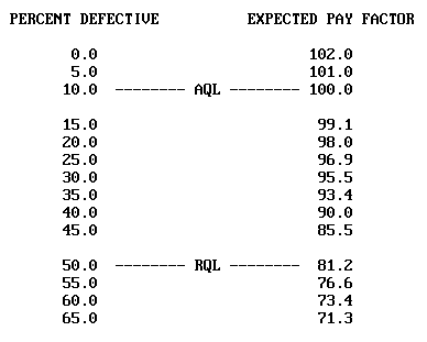
Figure M10. Display of Numerical Values of Points on EP Curve Computed
at High Precision by Program OCPLOT
Although the vast majority of highway construction measures tend to be normally distributed, there are some that are not. A physical constraint close to the desired target value often produces nonnormality. For example, depth of cover over the top mat of reinforcing steel in a bridge deck may tend to be skewed because it is physically impossible (provided the steel is embedded) for the cover to be less than zero but there is less of a restriction on how deep the mat might be. Similarly, if the target level for percent air voids in bituminous pavement is fairly low, the physical limit of zero may tend to skew this distribution toward larger values. Another condition that can produce nonnormality is the combining in the same lot of two distinctly different populations. As a general rule, a conscious effort should be made to avoid this condition when applying a statistical specification.
Because situations may arise in highway construction that warrant their use, program OCPLOT provides the capability of analyzing attributes acceptance procedures. Although it would be possible to develop a payment schedule based on an attributes procedure, their use has been limited almost exclusively to pass/fail applications. The following is presented as a generic example of such a procedure.
It is assumed for this example that the statistical quality measure is the percent defective (PD), the percentage of the lot falling outside specification limits. The acceptable quality level (AQL) and the rejectable quality level (RQL) are defined as PD = 10 and PD = 50, respectively. It is desired to develop an acceptance procedure that will balance the risks at 0.05. In other words, if the contractor provides work that is exactly at the AQL, there is to be a 0.05 chance that it will erroneously be rejected and, at the other extreme, if the work is truly at the RQL, there is to be a 0.05 chance that it will erroneously be accepted.
An acceptance plan is required, stated in terms of the sample size (N) and the acceptance number (C) that will produce the desired risks. For both risks to be 0.05, an OC curve is desired that indicates probabilities of acceptance at the AQL and the RQL of 0.95 and 0.05, respectively. Because both N and C must be integer values, the resultant risk levels vary in discrete steps, and it usually is not possible to obtain exactly the desired risk values. To find a plan that matches the desired risk levels as closely as possible, it is necessary to examine several plans.
This can easily be accomplished with program OCPLOT by selecting "Pass/Fail" and "Attributes" from the opening menu, followed by other appropriate selections and ending with a trial combination of N and C. It is usually advantageous to make the first few runs at low precision (selected from the second menu) in order to speed up the trial"and"error process.
Figure M11 shows the completed menu for the initial try with N = 10 and C = 2 and figure
M12 shows the resulting acceptance probabilities obtained at high precision. It can be seen in figure M12 that the probability of acceptance of 0.052 at the RQL is close to the desired value, while the probability of acceptance of 0.927 at the AQL is too low.
|
ENTER THE FOLLOWING INFORMATION |
|
ACCEPTANCE METHOD REJECTABLE QUALITY LEVEL Pass/Fail PD = 50 TYPE OF PROCUDURE RETEST PROVISION Attributes None QUALITY MEASURE SAMPLE SIZE Percent Defective 10 LIMIT TYPE ACCEPTANCE NUMBER SingleSided 2 ACCEPTABLE QUALITY LEVEL PD = 10 Press any key to continue |
|
<ESC> = Back <END> = Exit |
Figure M11. Completed Menu for Analysis of Pass/Fail Attributes
Acceptance Plan with N = 10 and C = 2
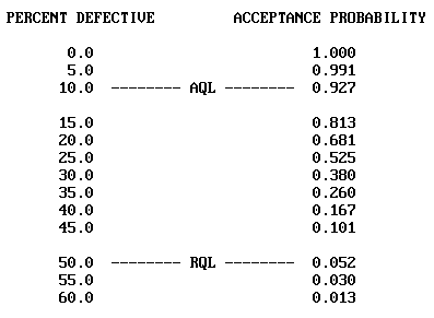
Figure M12. Numerical Values of Points on EP Curve for Pass/Fail Attributes Acceptance Plan with N = 10 and C = 2
The results of several attempts are presented in table M2. The values in this table were all obtained at high precision and here it can be seen that the plan having N = 13 and C = 3 comes the closest to meeting the desired acceptance probabilities of Prob. ³ 0.95 and Prob. £ 0.05 at the AQL and RQL, respectively. This is a trial and error process, but, with a little experience, it usually is possible to find a suitable plan relatively quickly.
|
Percent Defective (PD) |
Probability of Acceptance |
|||
N = 10 C = 2 |
N = 12 C = 3 |
N = 13 C = 3 |
N = 14 C = 3 |
|
|
0 |
1.000 |
1.000 |
1.000 |
1.000 |
|
10 (AQL) |
0.927 |
0.975 |
0.966 |
0.960 |
|
20 |
0.681 |
0.810 |
0.747 |
0.698 |
|
30 |
0.380 |
0.491 |
0.430 |
0.350 |
|
40 |
0.167 |
0.226 |
0.163 |
0.130 |
|
50 (RQL) |
0.052 |
0.079 |
0.048 |
0.028 |
|
60 |
0.013 |
0.014 |
0.006 |
0.011 |
The attributes acceptance plan meeting the requirements of this example requires that a total of N = 13 test specimens be taken from random locations within each lot and that, after the appropriate tests have been performed, no more than C = 3 of the test results shall be outside specification limits. The use of such a plan ensures that truly AQL work will be accepted about 95 percent of the time and that truly RQL work will be accepted only about 5 percent of the time.
Variables procedures are based on the assumption that the population being sampled is at least approximately normally distributed. They involve the computation of statistical parameters, such as the mean and standard deviation, to estimate PD or PWL. Provided the normality assumption is sufficiently well satisfied, variables procedures can provide essentially the same discriminating power as equivalent attributes plans, but with a substantially smaller sample size.
To illustrate this last statement, a variables procedure is sought that will have essentially the same discriminating power (OC curve) as the attributes procedure developed in example M1. Like the previous example, this involves a trial and error process with which program OCPLOT can be extremely helpful. For this example, the selections "Pass/Fail" and "Variables" are made from the opening menu, followed by other appropriate selections and ending with trial values for the sample size and acceptance limit.
This trialanderror process proceeds more quickly if a low level of precision is selected for the initial attempts. When it appears that the appropriate combination of sample size and acceptance limit has been found, this should be checked at intermediate precision. Further minor adjustments may then be necessary before confirming the result at high precision.
Figure M13 shows the completed menu for the variables acceptance plan that was ultimately selected. The actual numerical values on the OC curve are shown in table M3, which summarizes the results of examples M1 and M2. In this table it can be seen that the performance of the variables plan very closely matches that of the attributes plan in example M1 (table M2, N = 13, C = 3). The dramatic difference is that this has been accomplished with a sample size of N = 8, whereas the attributes plan required a sample size of N = 13. In this case, which assumes that the normality assumption is satisfied, the use of a variables plan results in a direct savings in sampling and testing costs of nearly 40 percent.
|
ACCEPTANCE METHOD REJECTABLE QUALITY LEVEL Pass/Fail PD = 50 TYPE OF PROCUDURE RETEST PROVISION Variables None QUALITY MEASURE SAMPLE SIZE Percent Defective 8 LIMIT TYPE ACCEPTANCE LIMIT SingleSided PD = 26 ACCEPTABLE QUALITY LEVEL PD = 10 Press any key to continue |
|
<ESC> = Back <END> = Exit |
Figure M13. Completed Menu for Pass/Fail Variables Acceptance Plan Example
|
Percent Defective |
Probability of Acceptance |
|
|
Attributes Plan |
Variables Plan |
|
|
0 |
1.000 |
1.000 |
|
5 |
0.997 |
0.996 |
|
10 (AQL) |
0.966 |
0.954 |
|
15 |
0.884 |
0.841 |
|
20 |
0.744 |
0.693 |
|
25 |
0.596 |
0.544 |
|
30 |
0.430 |
0.376 |
|
35 |
0.279 |
0.256 |
40 |
0.163 |
0.157 |
45 |
0.091 |
0.088 |
50 (RQL) |
0.048 |
0.048 |
55 |
0.024 |
0.024 |
60 |
0.006 |
0.009 |
Although the pass/fail acceptance procedures discussed in examples M1 and M2 may be useful for highway construction applications, the use of acceptance procedures with adjusted payment schedules is generally of greater interest. The proper design of such plans is critical to their performance, and poorly conceived plans may be either totally ineffective or impractically severe. Neither problem may be apparent, however, until the plan has been analyzed by constructing the EP curve.
Equation M1 gives a payment schedule proposed for use by an owner. The AQL was defined as PWLSPEC = 90 and, since there was no incentive payment provision, the maximum payment factor was limited to 100 percent.
PR = PWL SPEC PWLCOMP |
(M1) |
where: PR = payment reduction (percent).
PWLSPEC = specified PWL at the AQL.
PWLCOMP = PWL computed from test values.
To transform this equation into a form that can be handled by program OCPLOT, it is necessary to express it in terms of the payment factor rather than the payment reduction. By substituting PWLSPEC = 90 and PR = 100 PF into equation M1, equation M2 is obtained, subject to the restriction that PF £ 100.
PF = 10 + PWLCOMP |
(M2) |
where: PF = payment factor (percent)
PWLCOMP = PWL computed from test values.
To judge the effectiveness of this payment equation, the EP curve will be developed for a typical sample size of N = 5. The completed input menu is shown in figure M14. Following this, an intermediate level of precision was selected from the second menu to obtain the display at the AQL shown in figure M15. Finally, the program was run at high precision, which produced the displays shown in figures M16 and M17.
|
ACCEPTANCE METHOD ACCEPTABLE QUALITY LEVEL Pay Adjustment PWL = 90 QUALITY MEASURE REJECTABLE QUALITY LEVEL Percent Within Limits PWL = 50 LIMIT TYPE RQL PROVISION SingleSided None PAY EQUATION RETEST PROVISION PF = 10 + 1 PWL None MAXIMUM PAY FACTOR SAMPLE SIZE PF = 100 5 Press any key to continue |
|
<ESC> = Back <END> = Exit |
Figure M14. Completed Menu for Analysis of Payment Equation
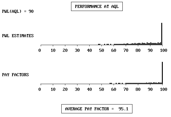
Figure M15. Performance of Payment Equation at AQL
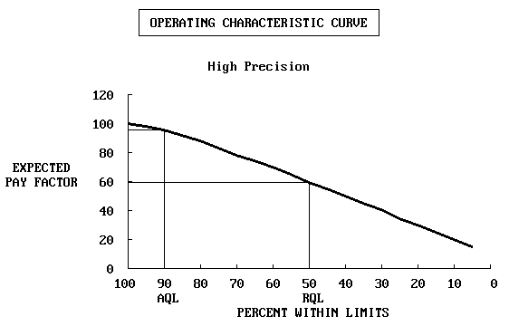
Figure M16. EP Curve for Analysis of Payment Equation
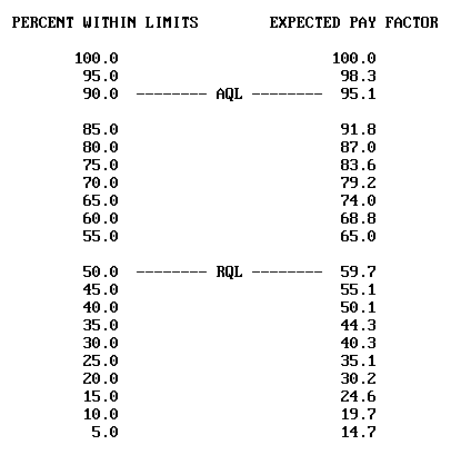
Figure M17. Numerical Values for Points on EP Curve for
Analysis of Payment Equation
It can be seen in figure M15 that there is a serious problem with this acceptance procedure. A contractor who performs consistently at the AQL will receive an average payment reduction of nearly 5 percent. To emphasize the impact this would have on the construction industry, this means that a contractor responsible for $10 million worth of work under this specification over the course of a construction season would on the average be penalized approximately $500,000 for successfully providing the level of quality that was explicitly defined as acceptable in the contract documents.
This example illustrates the situation discussed previously, whereby the failure to include an incentive payment provision with this type of specification prevents the acceptance procedure from paying an average of 100 percent when the work is exactly at the AQL. The reason for this can be seen with the help of figure M15. The upper histogram in this figure represents the distribution of 1000 PWL estimates, each obtained by randomly sampling a population that is exactly of AQL quality. These sample PWL estimates range from a low of about 47 percent to a high of 100 percent because of the inherent variability of the sampling process. However, the longterm average of these estimates will always be extremely close to the true value (the AQL in this case) because the PD/PWL estimation process is an unbiased statistical estimation procedure. The problem arises because the payment schedule does not permit this unbiased property to extend to the distribution of payment factors. Because there is no incentive payment provision, all PWL estimates that are greater than the true PWL of 90 receive the maximum payment factor of 100 percent, while all those below the true value receive some degree of payment reduction. Since approximately half the lots will receive payment reductions and the other half will receive 100 percent payment, the net result is that the average payment factor for AQL work will be substantially lower than 100 percent.
This situation is clearly misleading and unfair, yet it exists in current QA specifications. It is not difficult to correct, however, as demonstrated in the next example.
The problem described in the preceding example, in which truly AQL work receives a substantial payment reduction, is easy to correct. All that is required is the inclusion of an incentive payment provision as part of the acceptance procedure. In equation M2, this would mean removing the restriction that the maximum payment factor cannot exceed 100 percent.
Ordinarily, the maximum payment factor and the slope of the payment equation should be consistent with established (or estimated) performance relationships and the anticipated economic consequences of any departures from the specified AQL. To be consistent with this example, a maximum incentive payment factor of 110 percent will have to be used. In actual practice, however, most agencies have used incentive payment provisions of 105 percent or less.
To confirm that this will solve the problem, program OCPLOT was run an additional time with the identical input used for example M3 except that when the prompt "MAXIMUM PAY FAC TOR" appeared, selection 2 was chosen, indicating that no upper limit is placed on the payment equation. The program then automatically computed and displayed the maximum payment factor of PF = 110.0, as shown in the completed menu in figure M18. The performance at the AQL is displayed in figure M19, where it is seen that the expected payment factor is 100 percent, as desired.
|
ACCEPTANCE METHOD ACCEPTABLE QUALITY LEVEL Pay Adjustment PWL = 90 QUALITY MEASURE REJECTABLE QUALITY LEVEL Percent Within Limits PWL = 50 LIMIT TYPE RQL PROVISION Single-Sided None PAY EQUATION RETEST PROVISION PF = 10 + 1 PWL None MAXIMUM PAY FACTOR SAMPLE SIZE PF = 110.0 5 Press any key to continue |
|
<ESC> = Back <END> = Exit |
Figure M18. Completed Menu for Analysis of Acceptance Procedure with Incentive Payment Provision |
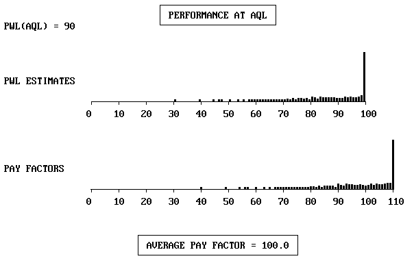
Figure M19. Performance at AQL of Acceptance Procedure with
Inventive Payment Provision
It was shown in chapter 7 that multiple OC curves could be plotted to illustrate the performance of acceptance plans with payment adjustment provisions. Each of these curves is associated not with the probability of acceptance, but with the probability of receiving greater than or equal to a given payment level. For example, suppose that equation M3 is selected to determine the payment for a lot based on a sample of size N = 5.
| PF = 55 + (0.5 x PWL) | (M3) |
From this equation it can be seen that full payment, i.e., PF = 100 percent, is obtained for a computed lot PWL of 90. Lot PWL values greater than 90 will lead to an incentive payment, while lot PWL values less than 90 will lead to a disincentive payment.
The probability of receiving a payment greater than or equal to 100 percent therefore is equivalent to the probability of receiving an individual estimated lot PWL of 90 or greater. By using the Pass/Fail option and selecting 90 as the ACCEPTANCE LIMIT, the OCPLOT program can be used to determine this OC curve. The completed OCPLOT menu for this situation is shown in figure M20, and the corresponding OC curve is shown in figure M21.
| ACCEPTANCE METHOD | REJECTABLE QUALITY LEVEL |
| Pass/Fail | PWL=50 |
| TYPE OF PROCEDURE | RETEST PROVISION |
| Variables | None |
| QUALITY MEASURE | SAMPLE SIZE |
| Percent Within Limits | 5 |
| LIMIT TYPE | ACCEPTANCE LIMIT |
| Single-Sided | PWL=90 |
| ACCEPTABLE QUALITY LEVEL | |
| PWL=90 | |
Press any key to continue |
|
| <ESC> = Back | <END> = Exit |
Figure M20. Completed Menu for Using OCPLOT to Determine the Probability of Receiving Greater than or Equal to 100 Percent Payment for Example M5 | |
Similarly, the probability of receiving greater than or equal to 95 percent payment is equivalent to the probability of receiving an individual estimated lot PWL of 80 or greater (obtained by plugging PF = 90 into equation M3 and solving for PWL). OCPLOT can once again be used with the Pass/Fail option and with 80 as the ACCEPTANCE LIMIT to determine this OC curve. This can be repeated for other payment levels to develop the family of OC curves shown in figure M22.
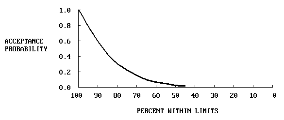
Figure M21. OC Curve for the Probability of Receiving Greater than or Equal
to 100 Percent Payment for Example M5
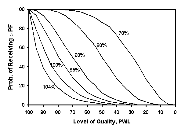 |
Figure M22. Family of OC Curves Showing the Performance of the Acceptance |