U.S. Department of Transportation
Federal Highway Administration
1200 New Jersey Avenue, SE
Washington, DC 20590
202-366-4000
Federal Highway Administration Research and Technology
Coordinating, Developing, and Delivering Highway Transportation Innovations
 |
| This report is an archived publication and may contain dated technical, contact, and link information |
|
Publication Number: FHWA-HRT-04-046 Date: October 2004 |
Previous | Table of Contents | Next
The quality index, which is used to estimate PD (or PWL), is calculated from the sample mean and standard deviation. Let us assume that the sample standard deviation is constant. This is not true; however, it allows us to show a simplified illustration of the effect that the variability of the sample mean can have on the estimated PD (or PWL) value. The top plot in figure 98 shows a normal distribution (skewness coefficient = 0) with 10 percent below the lower specification limit.
The two solid-line plots in the figure illustrate the distribution of the sample means for a sample size of n = 3. The distribution of the sample means will be centered at the population mean, while the standard deviation of the distribution of the sample means (known as the standard error) will be equal to ![]() , where σ is the population standard deviation. Therefore, the sample means will vary less than the original population from which they are drawn.
, where σ is the population standard deviation. Therefore, the sample means will vary less than the original population from which they are drawn.
The distribution with the dashed line in the middle plot represents, for a sample size of n = 3, a normal distribution with the smallest mean that can be obtained from the original population (once again simplifying by saying that the normal distribution only extends 3 standard deviations on either side of the mean). It shows that it is possible to get an estimated PD value of greater than 50 (or a PWL of less than 50) even though the actual PD value for the population is 10 (the actual PWL is 90). The distribution with the dashed line in the bottom plot represents, for a sample size of n = 3, a normal distribution with the largest mean that can be obtained. It shows that it is possible to get an estimated PD value as small as zero (a PWL of 100) even though the actual PD value for the population is 10 (the PWL is 90).
These results are relatively consistent with the values shown in the bias histograms in chapter 6 and appendix G. The histograms in figure 32 indicate that a bias value of +90 was obtained. This indicates that a PD estimate of 100 was obtained during the simulation. The reason that the plot in figure 98 does not allow for a value this large is that, in developing figure 98, it was assumed that the standard deviation was constant. Therefore, the dashed-line distributions have the same spread as the original population. In reality, the sample standard deviation also varies and, therefore, it is possible to obtain a very low sample mean and, on the same lot, a very low sample standard deviation. This combination could result in an estimated distribution that lies entirely below the specification limit.
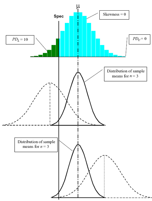
Figure 98. Spread of possible sample means for a normal distribution with 10 PD below the lower specification limit and sample size = 3.
The plots in figure 99 illustrate the same population as in figure 98, but with a sample size of n = 10. The larger sample size indicates that the distribution of the sample means will have less spread than that for a sample size of n = 3. It is still possible to have an estimated PD value of greater than 50; however, as drawn with the constant standard deviation, it would not be possible to have a PD estimate as low as zero. Once again, remember that these simplified examples assume that the standard deviation does not vary and remains equal to the population's standard deviation. They do, however, illustrate how natural sampling variability will lead to variability in the estimated PD (or PWL) values.
The remaining figures in appendix F illustrate different PDL/PDU divisions and different population PD values for the cases of symmetrical distributions (skewness = 0) and for skewed distributions (skewness coefficient = 1.0). They can be interpreted in the same way as the discussions for figures 98 and 99.
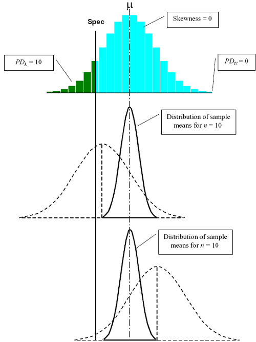
Figure 99. Spread of possible sample means for a normal distribution with 10 PD below the lower specification limit and sample size = 10.
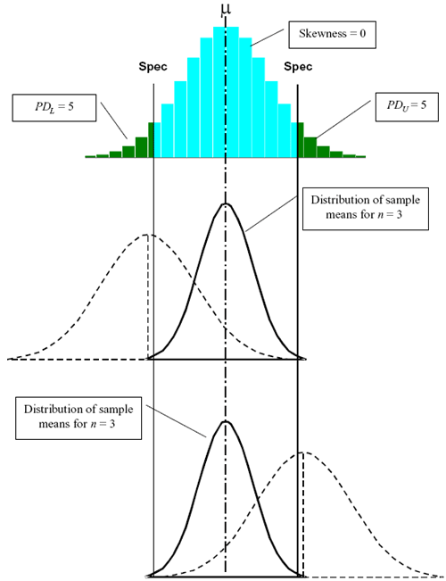
Figure 100. Spread of possible sample means for a normal distribution with 5 PD outside each specification limit and sample size = 3.
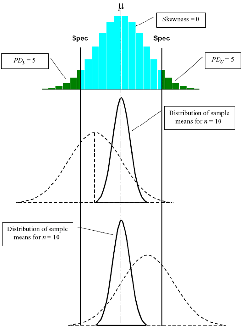
Figure 101. Spread of possible sample means for a normal distribution with 5 PD outside each specification limit and sample size = 10.
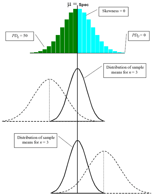
Figure 102. Spread of possible sample means for a normal distribution with 50 PD below the lower specification limit and sample size = 3.
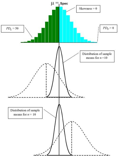
Figure 103. Spread of possible sample means for a normal distribution with 50 PD below the lower specification limit and sample size = 10.
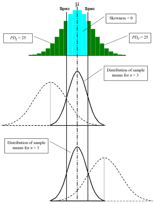
Figure 104. Spread of possible sample means for a normal distribution with 25 PD outside each specification limit and sample size = 3.
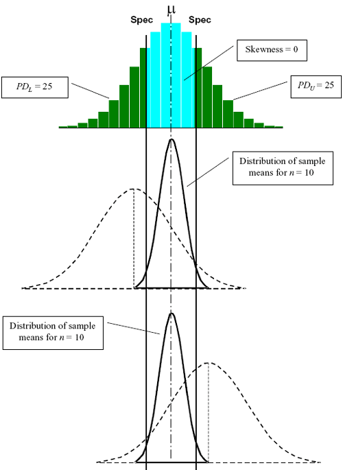
Figure 105. Spread of possible sample means for a normal distribution with 25 PD outside each specification limit and sample size = 10.
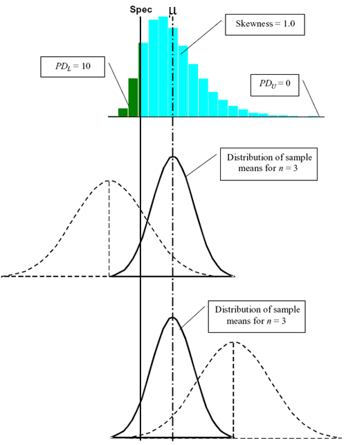
Figure 106. Spread of possible sample means for a distribution with skewness = 1.0, 10 PD below the lower specification limit, and sample size = 3.
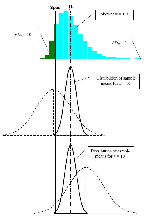
Figure 107. Spread of possible sample means for a distribution with skewness = 1.0, 10 PD below the lower specification limit, and sample size = 10.
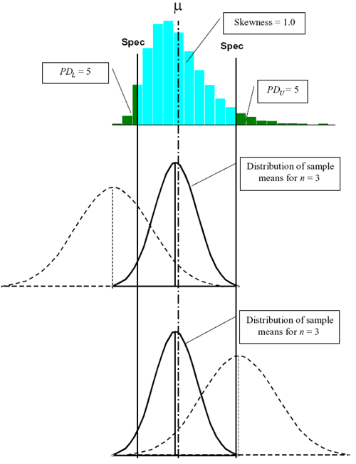
Figure 108. Spread of possible sample means for a distribution with skewness = 1.0, 5 PD outside each specification limit, and sample size = 3.
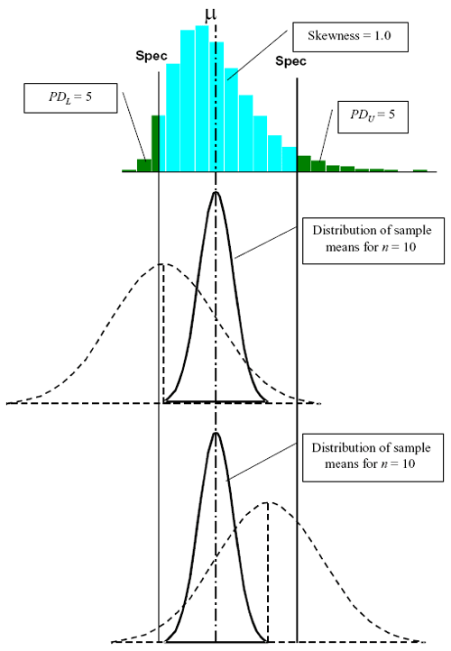
Figure 109. Spread of possible sample means for a distribution with skewness = 1.0, 5 PD outside each specification limit, and sample size = 10.
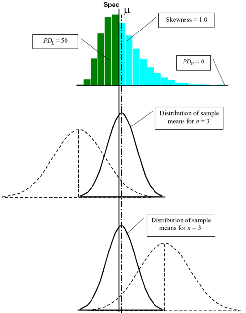
Figure 110. Spread of possible sample means for a distribution with skewness = 1.0, 50 PD below the lower specification limit, and sample size = 3.
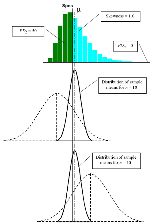
Figure 111. Spread of possible sample means for a distribution with skewness = 1.0, 50 PD below the lower specification limit, and sample size = 10.
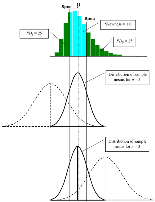
Figure 112. Spread of possible sample means for a distribution with skewness = 1.0, 25 PD outside each specification limit, and sample size = 3.
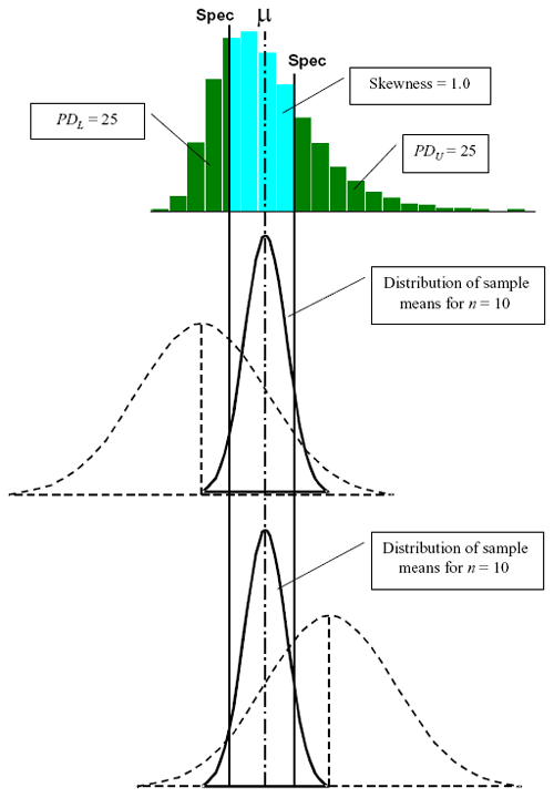
Figure 113. Spread of possible sample means for a distribution with skewness = 1.0, 25 PD outside each specification limit, and sample size = 10.

