Appendix E: Finite-Difference Temperature Model Validation

Previous | Table of Contents | Next

The HIPERPAV II temperature model predicts the temperature development of concrete at early ages. The temperature development in the concrete structure is determined by the balance between heat generation in the concrete and heat exchange with the environment. This model includes the heat of hydration of the cementitious materials and the heat transfer mechanisms of thermal conduction, convection (including evaporative cooling), solar radiation, and irradiation. In section B.1.2, all the models and material properties necessary to predict the temperature distribution in the pavement structure were presented.

Over the course of its development, HIPERPAV has employed two different temperature prediction models. Originally, the temperature prediction model was a transient two-dimensional FEM. However, this procedure required excessive solution times. The model has since been replaced by a one-dimensional finite-difference approach, which allows quicker execution without a compromise in accuracy. However, the accuracy of the finite-difference model needs to be verified by comparison with field data.

The model was calibrated by comparing the predicted versus measured field temperatures. To validate the temperature model, the concrete temperatures measured in the field were compared to the concrete temperatures predicted with the temperature model. Early-age temperature data were collected from PCC paving applications located across the United States. Eighteen slabs were instrumented; nine of these were selected for calibration and nine for validation of the model. Table 92 provides a brief summary of the different sites, and it also indicates which slabs will be used for the model calibration and validation.

E.1 Field Instrumentation Sites

Two separate mechanisms are considered to predict changes in pavement temperature: environmental effects and the PCC heat of hydration. Environmental conditions, including air temperature, solar radiation, windspeed, and relative humidity, were monitored by using a portable weather station. The heat of hydration over time of the cementitious materials was determined by adiabatic calorimeter testing. Concrete temperatures during the first 72 hours after concrete placement were measured with thermocouples installed at various depths: at 25 mm from the top, middepth, and 25 mm from the bottom of each slab. At some sites, concrete temperatures were recorded by free vibrating strain gauges located at the three depths described above.

Many parameters influence the development of concrete temperatures. During the field instrumentation, these parameters were measured or recorded in the field or obtained through laboratory tests, and these parameters are summarized in table 93. In addition to this information, the results of the cement heat of hydration tests and the properties used to model the boundary conditions and heat transfer for all the concrete mixes is listed in table 94.

Based on the data collected for these paving projects, the ranges of values covered during this calibration and validation effort are as follows:

• Pavement thickness: 200 to 305 mm.
• Subbase type: unbound granular, AC, and crushed concrete base.
• Cement type: I, IP, II, and I/II.
• Admixtures: 7 percent to 21 percent cement replacement with Class C fly ash and, 18 percent to 23 percent cement replacement with Class F fly ash.
• W/cm: 0.36 to 0.44 and w/c: 0.45 to 0.56.
• The air temperature during the instrumentation varied as follows: Minnesota 0.5 to 22 °C, Arizona -1.1 to 23 °C, Texas (Lufkin) 8 to 30 °C, North Carolina 8 to 28 °C, and Texas (Fort Worth) 25 to 37 °C. In general, the paving conditions for Minnesota and Arizona were colder than for the rest of the States.
• Curing method: White liquid curing compound was used at most of the sites. However, due to cold weather conditions in Arizona, polyethylene sheets were used to retain concrete temperatures during the first and second days after placement.

E.2 Model Calibration

The temperature model was calibrated by comparing the predicted versus measured concrete temperatures during the first 72 hours after placement. It was determined that some parameters had to be adjusted to calibrate the finite-difference model. After all the concrete temperatures from all the sites were evaluated against the predicted values, it is recommended that the following modifications be made to the temperature model:

• Solar absorptivity constant: The solar absorptivity of PCC is a function of the surface color, with typical values ranging from 0.5 to 0.6. An ideal white body would have a value of 0.0, and an ideal black body would have a value of 1.0. A solar absorptivity constant of 0.50 was found most appropriate for concrete pavements cured with white curing compound.
• Heat transfer by convection/conduction: The model outlined in section B.1.2.3 provides an accurate means to model the heat loss on the pavement surface. During the construction of the Arizona pavement, plastic sheets were used. Using the thickness of the plastic sheet and its thermal conductivity underestimated the amount of heat being retained by the pavement. However, when sheets are used, they are not in total contact with the slab, and the air void between the concrete and sheets act as additional insulation. An average air void thickness of 5 mm in addition to the plastic sheet provided an accurate account of the surface insulation for all the slabs where sheets were used. It is recommended that an additional air void thickness of 5 mm be used for all future cases where plastic sheets are used.
• Heat transfer due to evaporative cooling: When evaporation of the water from a surface occurs, the energy associated with the phase change is the latent heat of vaporization, which causes evaporative cooling. A preliminary model to account for heat transfer due to evaporative cooling was developed.⁽¹²²⁾ The use of the model depends on the interaction between curing, bleeding, and environmental conditions. These effects were noticeable only for some of the slabs in North Carolina . This is an area where further research is required to model the interaction between moisture movement, bleeding, concrete materials, curing compound effectiveness, and evaporation.
• Solar radiation: The amount of heat gain due to solar radiation varies with longitude, latitude, altitude, time of day, day of year, and the prevailing atmospheric conditions. Next to the heat of hydration, the flux due to solar radiation is the most important heat source to the pavement system and should be modeled. In HIPERPAV II, the environmental data for any location in the United States are generated based on averaged 30-year historical data obtained from a weighted average of nearby weather stations. It is recommended that the hourly values from this database be used for the temperature prediction. The maximum solar flux may be determined as the 99^th percentile of the 30-year average hourly global horizontal radiation.
• Cloud cover: During day times, cloud cover affects the intensity of the direct and diffuse solar radiation that reaches the pavement surface. During night times, the cloud cover also determines the amount of reradiation from surfaces, and affects the magnitude of the irradiation. To achieve accurate temperature predictions, the amount of cloud cover should be defined as accurately as possible by the user.
• AE: The AE determines the temperature sensitivity of the concrete's hydration process relative to that at the reference temperature. The AE model described in section B.1.1 is recommended for use.
• Ultimate degree of hydration: Complete hydration of all the cementitious materials is seldom attained in actual concrete structures. This depends on the amount of space available for the hydration products, and also on the need for sufficient free mix water, which ensures continued hydration.^(123,124) The model described in section B.1.1 is recommended to determine the ultimate degree of hydration for saturated concrete.

Notes: * S - Sunny, PC - Partly Cloudy, C - Cloudy, OC - Overcast ** - Collected under HIPERPAV I validation *** - Collected under HIPERPAV II validation

^a Hydration parameters were determined by adiabatic calorimeter tests

The measured temperatures and the predicted temperatures for all the calibration sites are presented in figures 196 to 231 in section E.5. The goodness of the temperature prediction was calculated in terms of the coefficient of determination (r² value). The calculation of the r² value was also performed to the 45° line (measured versus predicted temperature). Two r² values were computed for each instrumented section:

• An average r² value obtained after comparing the temperatures at 25 mm from the top, middepth, and 25 mm from the bottom of each slab.
• An r² value obtained after comparing the measured versus predicted temperature differential.

The r² values obtained for the calibration sites are summarized in table 95. The average r² values ranged between 0.750 and 0.866. The r² values obtained for the temperature gradient ranged between 0.539 and 0.909. The low r² values were obtained for the JCP section instrumented in Texas . From the r² values obtained during this analysis, it may be concluded that the modified finite-difference model incorporated in HIPERPAV II is calibrated sufficiently. The model should be validated to determine the accuracy of the temperature prediction for PCC paving applications.

E.3 Model Validation

The measured versus predicted temperatures were compared as outlined in the previous section. The measured temperatures and the predicted temperatures for all the validation sites are presented in figures 232 to 267 in section E.6. The goodness of the temperature prediction was calculated in terms of the two r² values documented in the calibration section. The r² values obtained for the validation sites are summarized in table 96. The average r² values ranged between 0.803 and 0.903. The r² values obtained for the temperature gradient ranged between 0.470 and 0.924. As was the case for the model calibration, the lowest r² values were obtained for the JCP section instrumented in Texas.

From the r² values obtained during this analysis, it may be concluded that the finite-difference model included in HIPERPAV II provides an accurate prediction of early-age concrete temperatures for PCC paving applications.

E.4 Summary and Recommendations

The early-age temperature development of concrete can be estimated from knowledge of cement composition, cement factor, admixtures, thermal characteristics of the concrete, slab thickness, and the environmental conditions that occur during paving and curing. Based on the calibration of the temperature model, recommendations were made to adjust/modify some models. These include modifications to the solar absorptivity constant, heat transfer by convection when plastic sheet are used, heat transfer due to evaporative cooling, the maximum solar radiation intensity, AE, and the ultimate degree of hydration. Major findings from this investigation are as follows:

• Adiabatic calorimeter tests provide a means of characterizing concrete hydration with time. With the parameters determined through these tests, the temperature prediction model can account for the effects that different mixture proportions and constituents have on the heat of hydration of concrete.
• Heat transfer due to evaporative cooling may significantly reduce temperatures in hydrating concrete. A model to account for this effect has been developed, and it is recommended that this model be further developed to account for actual construction practices. Modeling of the moisture condition in the hardened cement paste will be beneficial for this purpose.
• From the high r² values shown in tables 95 and 96, and the temperature predictions shown in sections E.5 and E.6, it may be concluded that the finite-difference model is able to produce good predictions of the early-age concrete temperatures development in concrete paving applications.

E.5 Temperature Prediction Results Obtained During Calibration

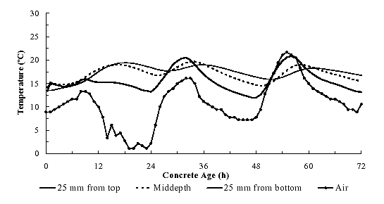
Figure 196. Measured concrete and air temperatures for Minnesota, Slab 1.

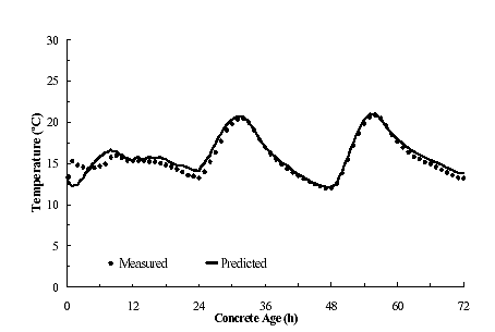
Figure 197. Measured versus predicted temperatures 25 mm from top of slab for Minnesota, Slab 1.

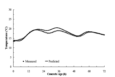
Figure 198. Measured versus predicted temperatures 25 mm from bottom of slab for Minnesota, Slab 1.

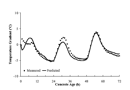
Figure 199. Measured versus predicted temperature gradient for Minnesota, Slab 1.

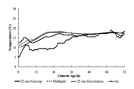
Figure 200. Measured concrete and air temperatures for Minnesota, Slab 4.

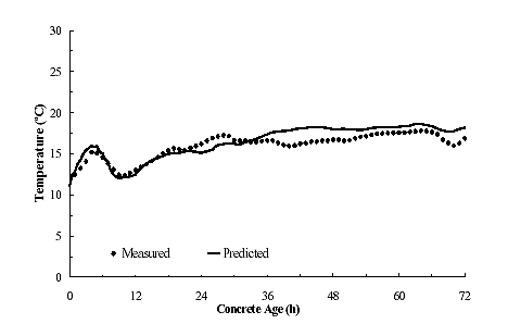
Figure 201. Measured versus predicted temperatures 25 mm from top of slab for Minnesota, Slab 4.

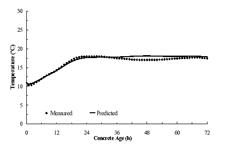
Figure 202. Measured versus predicted temperatures 25 mm from bottom of slab for Minnesota, Slab 4.

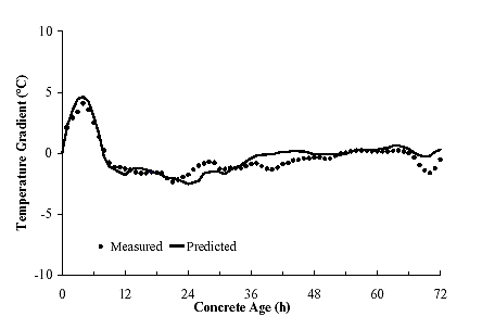
Figure 203. Measured versus predicted temperature gradient for Minnesota, Slab 4.

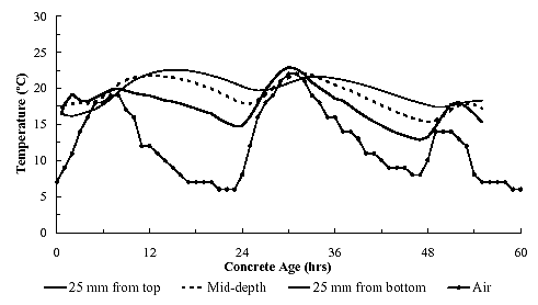
Figure 204. Measured concrete and air temperatures for Arizona, Slab 1.

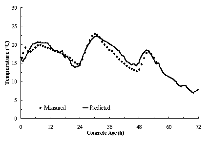
Figure 205. Measured versus predicted temperatures 25 mm from top of slab for Arizona, Slab 1.

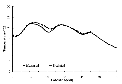
Figure 206. Measured versus predicted temperatures 25 mm from bottom of slab for Arizona, Slab 1.

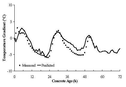
Figure 207. Measured versus predicted temperature gradient for Arizona, Slab 1.

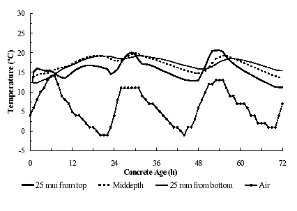
Figure 208. Measured concrete and air temperatures for Arizona, Slab 3.

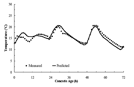
Figure 209. Measured versus predicted temperatures 25 mm from top of slab for Arizona, Slab 3.

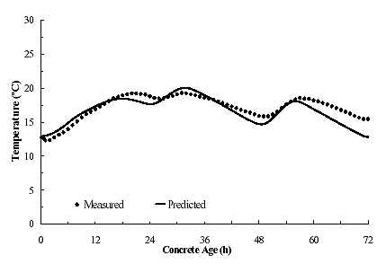
Figure 210. Measured versus predicted temperatures 25 mm from bottom of slab for Arizona, Slab 3.

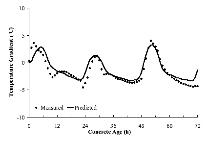
Figure 211. Measured versus predicted temperature gradient for Arizona, Slab 3.

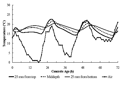
Figure 212. Measured concrete and air temperatures for Arizona, Slab 6.

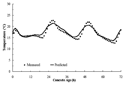
Figure 213. Measured versus predicted temperatures 25 mm from top of slab for Arizona, Slab 6.

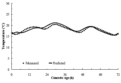
Figure 214. Measured versus predicted temperatures 25 mm from bottom of slab for Arizona, Slab 6.

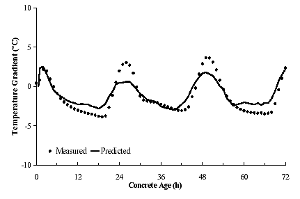
Figure 215. Measured versus predicted temperature gradient for Arizona, Slab 6.

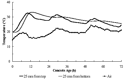
Figure 216. Measured concrete and air temperatures for Lufkin, TX, Slab 2.

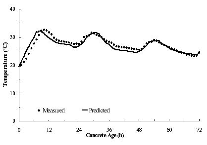
Figure 217. Measured versus predicted temperatures 25 mm from top of slab for Lufkin, TX, Slab 2.

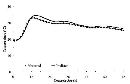
Figure 218. Measured versus predicted temperatures 25 mm from bottom of slab for Lufkin, TX, Slab 2.

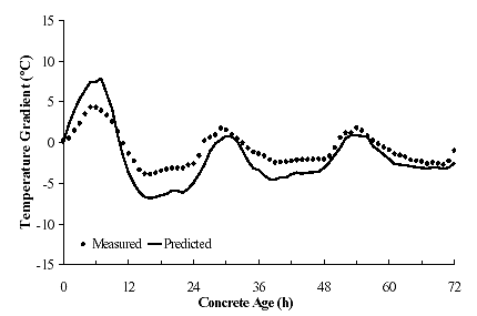
Figure 219. Measured versus predicted temperature gradient for Lufkin, TX, Slab 2.

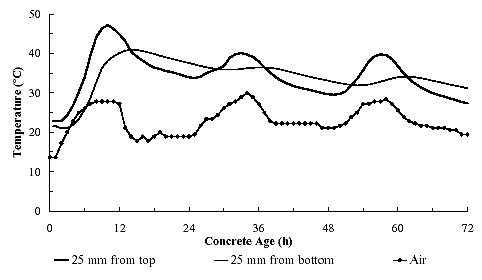
Figure 220. Measured concrete and air temperatures for Lufkin, TX, Slab 3.

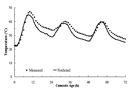
Figure 221. Measured versus predicted temperatures 25 mm from top of slab for Lufkin, TX, Slab 3.

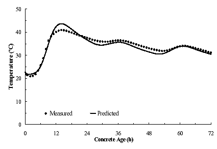
Figure 222. Measured versus predicted temperatures 25 mm from bottom of slab for Lufkin, TX, Slab 3.

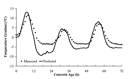
Figure 223. Measured versus predicted temperature gradient for Lufkin, TX, Slab 3.

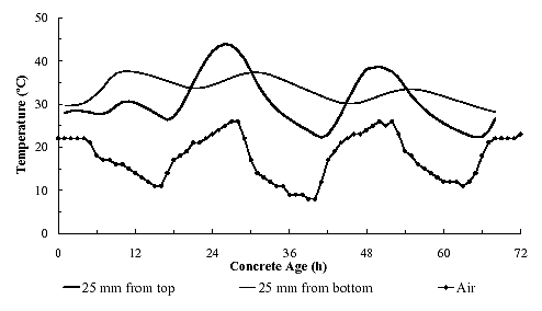
Figure 224. Measured concrete and air temperatures for North Carolina, Slab 2.

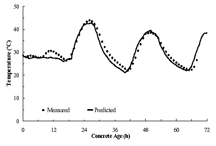
Figure 225. Measured versus predicted temperatures 25 mm from top of slab for North Carolina, Slab 2.

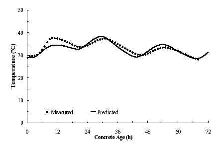
Figure 226. Measured versus predicted temperatures 25 mm from bottom of slab for North Carolina, Slab 2.

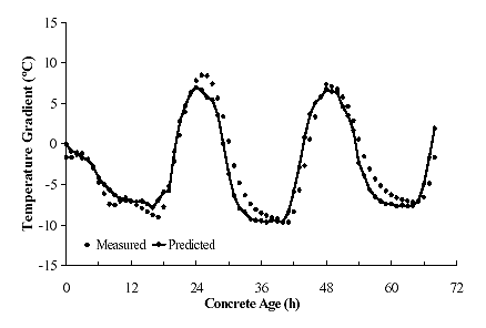
Figure 227. Measured versus predicted temperature gradient for North Carolina, Slab 2.

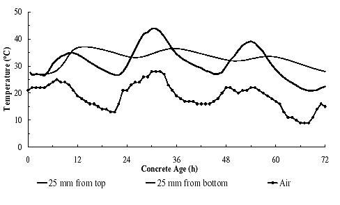
Figure 228. Measured concrete and air temperatures for North Carolina, Slab 3.

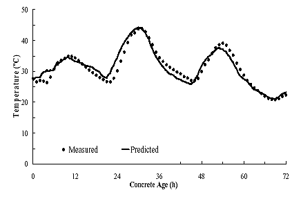
Figure 229. Measured versus predicted temperatures 25 mm from top of slab for North Carolina, Slab 3.

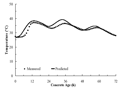
Figure 230. Measured versus predicted temperatures 25 mm from bottom of slab for North Carolina, Slab 3.

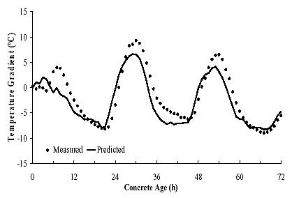
Figure 231. Measured versus predicted temperature gradient for North Carolina, Slab 3.

E.6 Temperature Prediction Results Obtained During Validation

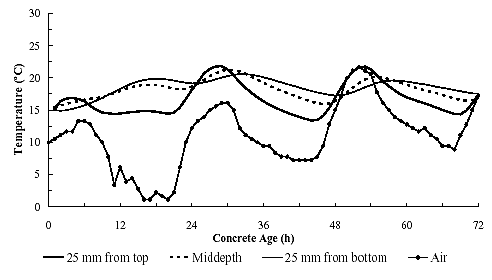
Figure 232. Measured concrete and air temperatures for Minnesota, Slab 2.

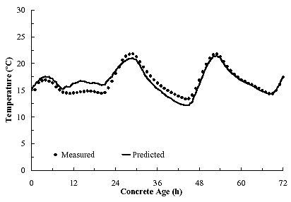
Figure 233. Measured versus predicted temperatures 25 mm from top of slab for Minnesota, Slab 2.

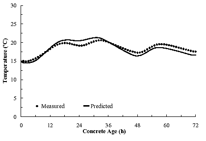
Figure 234. Measured versus predicted temperatures 25 mm from bottom of slab for Minnesota, Slab 2.

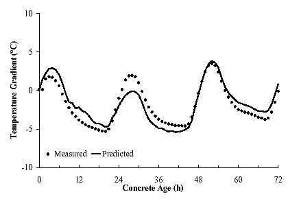
Figure 235. Measured versus predicted temperature gradient for Minnesota, Slab 2.

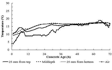
Figure 236. Measured concrete and air temperatures for Minnesota, Slab 3.

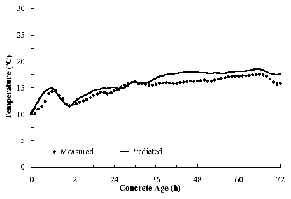
Figure 237. Measured versus predicted temperatures 25 mm from top of slab for Minnesota, Slab 3.

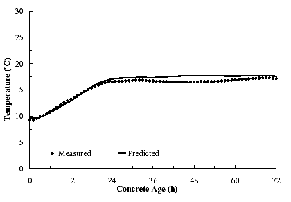
Figure 238. Measured versus predicted temperatures 25 mm from bottom of slab for Minnesota, Slab 3.

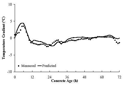
Figure 239. Measured versus predicted temperature gradient for Minnesota, Slab 3.

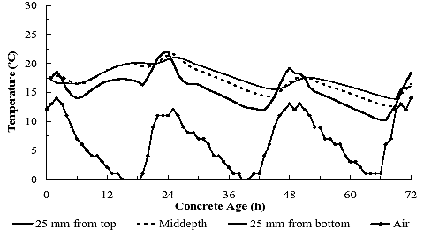
Figure 240. Measured concrete and air temperatures for Arizona, Slab 4.

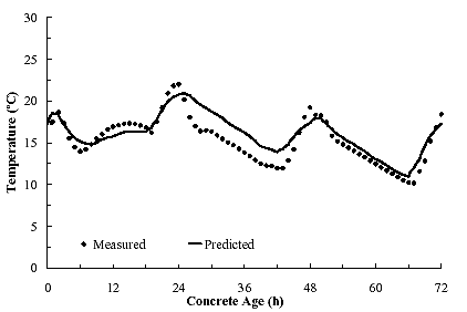
Figure 241. Measured versus predicted temperatures 25 mm from top of slab for Arizona, Slab 4.

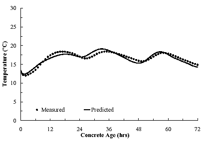
Figure 242. Measured versus predicted temperatures 25 mm from bottom of slab for Arizona, Slab 4.

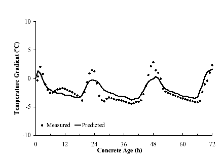
Figure 243. Measured versus predicted temperature gradient for Arizona, Slab 4.

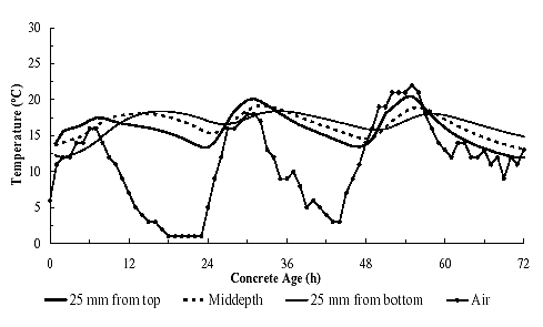
Figure 244. Measured concrete and air temperatures for Arizona, Slab 5.

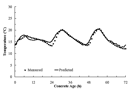
Figure 245. Measured versus predicted temperatures 25 mm from top of slab for Arizona, Slab 5.

Figure 246. Measured versus predicted temperatures 25 mm from bottom of slab for Arizona, Slab 5.

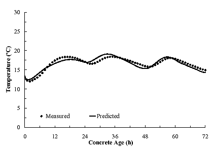
Figure 247. Measured versus predicted temperature gradient for Arizona, Slab 5.

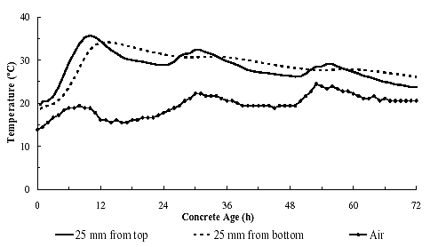
Figure 248. Measured concrete and air temperatures for Lufkin, TX, Slab 1.

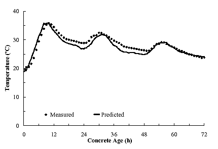
Figure 249. Measured versus predicted temperatures 25 mm from top of slab for Lufkin, TX, Slab 1.

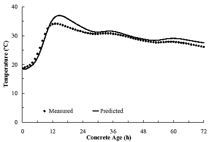
Figure 250. Measured versus predicted temperatures 25 mm from bottom of slab for Lufkin, TX, Slab 1.

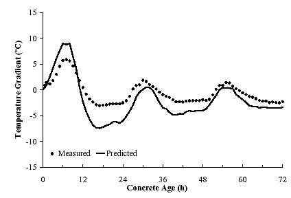
Figure 251. Measured versus predicted temperature gradient for Lufkin, TX, Slab 1.

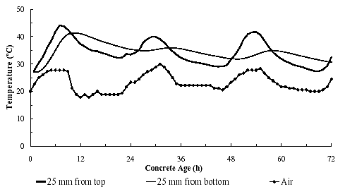
Figure 252. Measured concrete and air temperatures for Lufkin, TX, Slab 4.

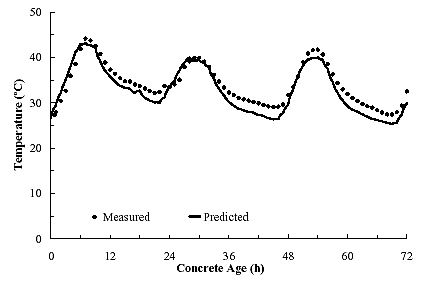
Figure 253. Measured versus predicted temperatures 25 mm from top of slab for Lufkin, TX, Slab 4.

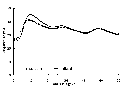
Figure 254. Measured versus predicted temperatures 25 mm from bottom of slab for Lufkin, TX, Slab 4.

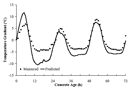
Figure 255. Measured versus predicted temperature gradient for Lufkin, TX, Slab 4.

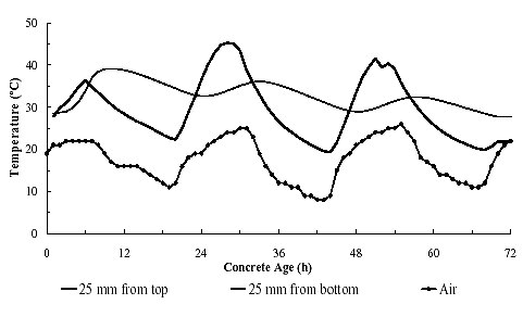
Figure 256. Measured concrete and air temperatures for North Carolina, Slab 1.

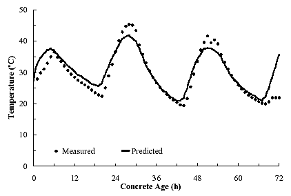
Figure 257. Measured versus predicted temperatures 25 mm from top of slab for North Carolina, Slab 1.

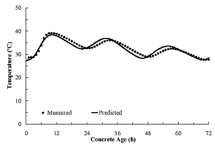
Figure 258. Measured versus predicted temperatures 25 mm from bottom of slab for North Carolina, Slab 1.

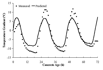
Figure 259. Measured versus predicted temperature gradient for North Carolina, Slab 1.

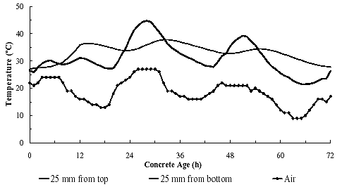
Figure 260. Measured concrete and air temperatures for North Carolina, Slab 4.

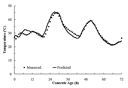
Figure 261. Measured versus predicted temperatures 25 mm from top of slab for North Carolina, Slab 4.

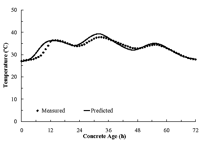
Figure 262. Measured versus predicted temperatures 25 mm from bottom of slab for North Carolina, Slab 4.

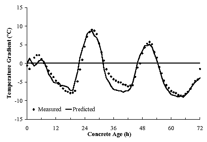
Figure 263. Measured versus predicted temperature gradient for North Carolina, Slab 4.

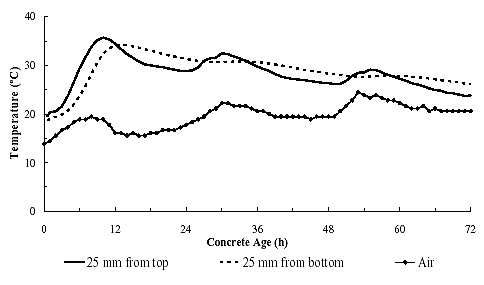
Figure 264. Measured concrete and air temperatures for Fort Worth, TX, Slab 1.

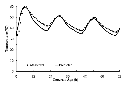
Figure 265. Measured versus predicted temperatures 25 mm from top of slab for Fort Worth, TX, Slab 1.

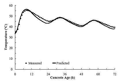
Figure 266. Measured versus predicted temperatures 25 mm from bottom of slab for Fort Worth, TX, Slab 1.

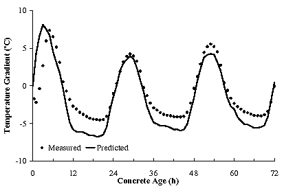
Figure 267. Measured versus predicted temperature gradient for Fort Worth, TX, Slab 1.