• Federal Highway Administration >
• Publications >
• Research Publications >
• 09044 >
• Chap7.Cfm >
• Integrity of Infrastructure Materials and Structures

Publication Number: FHWA-HRT-09-044
Date: October 2009

Previous | Table of Contents | Next

CHAPTER 7. RESEARCH APPROACH #2

TASK 2.1. LABORATORY TEST METHOD FOR PRODUCTION OF PROTECTIVE
AND NONPROTECTIVE OXIDE LAYERS IN CHLORIDE ENVIRONMENTS

Wet/Dry Cycle

The Society for Automotive Engineers (SAE) established an accelerated test under dry/wet conditions to test metal coatings under highly corrosive environment known as Standard SAE J-2334.⁽²⁴⁾ The test has been characterized as, "J2334 Best Correlation to 5-Year Data (Field) at 80–Cycles."⁽²⁵⁾ The cycle is shown in figure 16. The five-cycle per week option maintained the dry condition during weekends. The soak solution specified in the standard is 0.5 percent NaCl + 0.1 percent CaCl2 + 0.075 percent NaHCO₃.

Figure 16. Chart. Standard SAE J2334 cyclic test with five cycles/week.

Exposure Tests

Standard SAE J-2334 was the starting point for the first set test, and alternative soak solutions were used. The behaviors of the steels varied at different chloride compositions. Four chloride concentrations were selected for the salt application. The chloride concentrations ranged from no chloride to a 5-wt percent composition solution, corresponding to an environment with very high salt deposition similar to a bridge that undergoes regular salt deicing processes. To account for environments that were subject to acid rain, each chloride concentration was subdivided—one group had a pH 6 and the other had a pH 8. Time of wetness and chloride exposures played an important role in the corrosion of steel. To study the influences, half of the exposure environments included a second 15-minute salt soak 3 hours after the first one. Table 6 summarizes the compositions of the soak solutions.

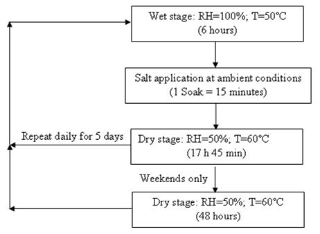
An environmental chamber manufactured by CARON^® Model 6030 was used for the experiment (see figure 17). The humidity and temperature inside the chamber were controlled and programmed. The wet stage started every day at 8 a.m. At 2 p.m., the dry stage started, and the first soak was performed. For the tests with two soaks, the second soak was performed at 5 p.m., 3 hours after the first one. There were 6 coupons of each steel type exposed to each solution, which created a total of 192 coupons for the entire experiment. Specifically, the 192 coupons were calculated by multiplying 2 steel types by 8 solutions by 2 soaking methods by 6 coupons (3 for 15 cycles plus 3 for 30 cycles). Weight losses were reported as the average of three specimens.

The 16 racks, fabricated from polyvinyl chloride (PVC) to accommodate 12 coupons each, were custom made for holding the coupons in the chamber (1 rack for each environment). Six coupons of each material were placed on each rack. One rack held six coupons of A606 steel and six coupons of SAE1010 steel. Two racks (24 coupons) were soaked in the same container. This arrangement allowed all coupons to be soaked within the same 15-minute time period. Images of a rack and soaking container are shown in figure 17 and figure 18.

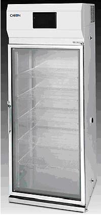
Figure 17. Photo. CARON^® environmental chamber for cyclic SAE J2334 tests.

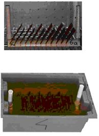
Figure 18. Photo. Specimens on holder rack and in soak tank.

After obtaining the data from this first set test (15 and 30 cycles), a second set test was carried out. These steels showed the most interesting behavior at chloride levels between zero and 2 wt percent. Based on the results of the first set test, a narrower and lower range of seven chloride concentrations was chosen in addition to 0.5-wt percent concentration as a reference point (reproduction). The second set test (15 and 30 cycles) was performed to obtain details in this concentration range. This time, only pH 8 was considered, and one soak was performed. Table 7 lists the different solutions used for the second set test.

For these experiments, 8 PVC racks held 12 coupons each (1 rack for each environment) with 6 coupons of each material. A set of 96 coupons was prepared for this second set test. The total number of coupons was calculated by multiplying 2 steel types by 8 solutions by 1 soaking method by 6 coupons (3 for 15 cycles and 3 for 30 cycles). Weight losses were reported as the average of three specimens.

Coupon Preparation

Very clean contaminant-free surfaces were needed for this experiment. The procedures to prepare the coupons follow.

A606 Steel

The1.5-mm thick material was cut to approximately 102-mm by 102-mm coupons. A 2.5-mm hole was drilled for the label attachment. The surface was bead blasted for 3 minutes on each side using type AC (60-120 mesh, 0.12-0.25-mm-diameter) type glass beads. The four sides were measured to assure squareness of the coupons and recorded. A label was attached consisting of a nylon zip tie engraved with the specimen identification. The specimens were dipped in methanol and drained on clean laboratory wipes. They were then dried with hot air for 2 minutes to prevent water condensation. The coupons were equilibrated in a desiccator for 1 hour, weighed, and stored in the desiccator until the beginning of exposure testing.

SAE1010 Steel

The 0.76-mm-thick material was cut to 76- by 102-mm coupons and prepared in the same manner described for the A606 material except bead blasting was required for only 1 minute per side.

Weight Loss

Data after 15 and 30 cycles of exposure were required for each of the 16 environments for the first set test. According to ASTM Standard G1 for evaluating corrosion rate, three coupons were needed for each weight loss measurement.⁽²⁶⁾ There were 6 coupons for each steel for the 16 environments (6 •2•16 = 192 coupons). After exposure, coupons were cleaned in a solution of hydrochloric acid, hexamethylenetetramine (inhibitor), and reagent water as specified in ASTM Standard G1.⁽²⁶⁾ The coupons were then dried and weighed.

X-ray Diffraction Analyses

After exposure, some corrosion products were collected before cleaning. For each environment and material, corrosion products were collected for X-ray diffraction (XRD) analysis. The corrosion products were then ground with mineral oil for powder analysis.

Powder XRD was performed on some of the corrosion products to characterize the correspondence between chamber condition and field exposure. A Philips^® Model PW1710 system with DiffTech^® Visual XRD control software was used for the measurements. The X-ray

The spectrum had a number of counts plotted versus angle of diffraction (see figure 19).

Software detected peaks from the spectrum, which were observed as significant increases in counting rate (intensity) in the figure. Each peak at a specific angle had a relative intensity associated. Two parameters (θ and I_x) were used to compare with a database. For this study, only peak angles and their associated relative intensities were required for crystallographic compound searches.

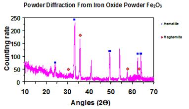
Figure 19. Graph. Example of X-ray powder diffraction spectrum.

The focus of this analysis was on four iron oxides identified during the on-site (field) exposure: goethite, akaganeite, lepidocrocite, and maghemite. A fifth compound, butlerite, was observed in the cable sensor study.⁽²⁷⁾ The database used for the comparison is the online edition of the American Mineralogist Crystal Structure Database.⁽²⁸⁾ Each crystalline configuration had numerous peaks, and a listing of all of them would be unnecessary because in the case of a mixture of several crystalline configurations, identifying the main two or three peaks via relative intensity was usually sufficient. The main reference angle peaks for an X-ray wavelength of 0.1541838 nm and associated intensities are presented in table 8.

The table lists the location (by angle) of the three largest peaks observed for each iron oxide and the relative intensity (peak) of each peak. The largest peak is taken as the reference (100 percent), and the remaining two peaks are listed as percentages of the largest peak. For example, if the largest peak has an intensity of 500 and the second peak has an intensity of 250, the relative intensities would be 100 and 50 percent, respectively. If a third peak for this compound has an intensity of 400, its relative intensity would be 80 percent. Determining which oxides are present in a sample requires examining the patterns for peaks at the angles where having 100-percent relative intensities and verifying the presence of secondary and tertiary peak angles are expected. Computer algorithms usually perform these functions.

TASK 2.2. CORROSION RATES OF ACCELERATED TEST SPECIMENS USING GALVANIC SENSORS

Approach

Galvanic corrosion sensors were developed to (1) react to humidity and chloride concentration, (2) be easily deployable on a steel structure, (3) give an indication of the corrosion rate of the structure, and (4) obtain data comparable with the data from the chamber exposure.

Sensor Design

Several primary designs were tested before selecting the final design described in figure 20 and figure 21.

When the sensor was exposed to high humidity, a meniscus formed on the edge of the insulating nylon washer, making an electrolytic connection between the steel and the cathode (copper or gold). Nylon polymer performed better than several other polymer materials evaluated for this sensor application. During galvanic corrosion, electrons moved to the cathode, producing a current, which was recorded by the data logger connecting the two external copper leads. When dry, no electrochemical reactions occurred, and no current (electrons) flowed. Intermediate conditions yielded moderate current values.

Preliminary studies showed that the electric connections and the seal between the insulating nylon washer anode and cathode required extra care. If water infiltrated under the washer, a crevice corrosion phenomenon was possible that provided alternate current paths that were not measurable by the data logger (errors).

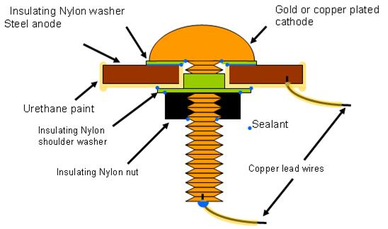
Figure 20. Illustration. Atmospheric corrosion sensor (Model FAU2).

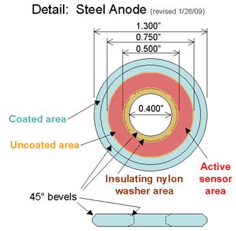
Figure 21. Illustration. Anode detail for atmospheric corrosion sensor.

The sensors were built with several elements. The center screw had a diameter of 6.6 mm with 20 threads per 25.4 mm by 25.4 mm long made of brass with copper or gold plating. The insulating nylon washers were machined from a 0.508-mm thickness Nylon 6/6 flat washer with a 6.6-mm inside diameter to 17.4-mm outside diameter, and a thickness of 0.508 mm. Both steel washers had a 33.02-mm outside diameter and a 10.16-mm inside diameter. The A606 steel washer (anode) was 1.52 mm thick, and the SAE1010 washer (alternate anode) was 0.762 mm thick. For SAE1010 sensors, an extra nylon shimming washer with a 9.906-mm inside diameter, a 15.748-mm outside diameter, and 6.890-mm thickness was used in between the shoulder washer and the steel washer. The shoulder washer was made of Nylon 6/6 with an inside diameter of 6.604 mm, an outside diameter of 9.525 mm, a shoulder diameter of 14.275 mm, and a thickness of 1.524 mm. Finally, nuts were Nylon 6/6 with matching-screw thread with a width of 11.11 mm across the flats and a height of 6.10 mm.

Zero Resistance Ammeter Data Logger

To obtain the data from the sensors, zero resistance ammeter (ZRA) loggers were developed.⁽¹⁴⁾ A zero resistance ammeter is an electronic device that converts current at its input into voltage at its output. This device imposes no (zero) voltage drop to the input circuit. It is designed to measure small currents (on the order of 1-100 µ A) without interfering with (polarizing) the circuit being measured. The ZRA was embedded in a data logger circuitry that acquired data every 10 minutes. The data were summed and stored every hour. It collected up to 2 months of data while powered by a single lithium 9V battery. The data loggers had a full range of 100 µ A. This maximum current was a design parameter for the sensors. The sensor output was intended to be limited to 100 γ A. A picture of a data logger is presented in figure 22.

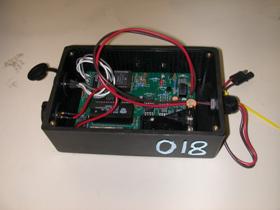
Figure 22. Photo. Data logger incorporating a ZRA.

The data was transferred from the data logger via a serial port to a computer in a hexadecimal format. A Microsoft Excel^® macro was used to transfer hexadecimal data to corrosion current values, and data could then be plotted normally in decimal format.

Sensor Active Area

As discussed previously, the sensors reacted to humidity and temperature. A flat steel surface seemed to be the best choice, representing the as-fabricated surface of a structure. It proved to be a simple and relatively cost-effective way to manufacture the sensor.

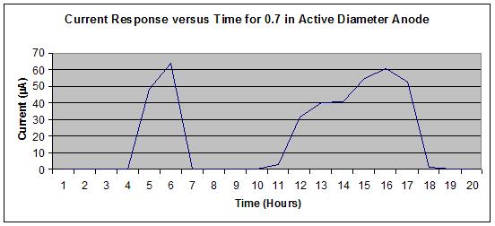
The current flowing between the two electrodes was limited to 100 µA during the wet cycle when the maximum currents occurred for optimal data acquisition by the logger. Because the anode surface was the controlling parameter, the surface area of the steel was limited in size to keep the output from exceeding the 100-µA value. The maximum corrosion rate was expected to decrease or stay constant with time, which permitted short duration exposure tests to be performed on simplified sensors to determine the optimal surface area.

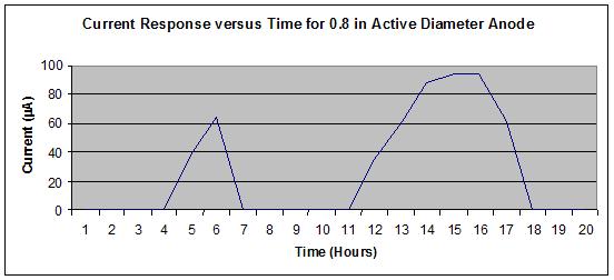
Figure 23 shows no off-scale output, whereas figure 24 shows a slight off-scale output (flattened peak) from the 16th to 17th hours during the wet portion of the J2334 cycle. To optimize the output range of the sensors, a 19.05-mm diameter active area was specified for the steel washer (anode) to allow use of a significant portion of the logging scale without exceeding the maximum value of 100 µ A.

1 inch = 25.4 mm
Figure 23. Graph. Sensor output for 0.7-inch active anode steel
washer diameter for one SAE J2334 cycle in the standard solution.

1 inch = 25.4 mm
Figure 24. Graph. Sensor output for 0.8-inch active anode steel washer diameter for
one SAE J2334 cycle in the standard solution.

For a flat surface desired for the sensors, a disk (washer) was fabricated and then painted (masked) to leave a circular area of bare steel at the center. The paint proved to be an issue during a previous test, as shown in figure 25. Under-paint corrosion occurred, and additional steel surface was subject to corrosion, giving undesirable results. Later, urethane-based powder coating was selected because of its excellent corrosion resistance and salt tolerance.

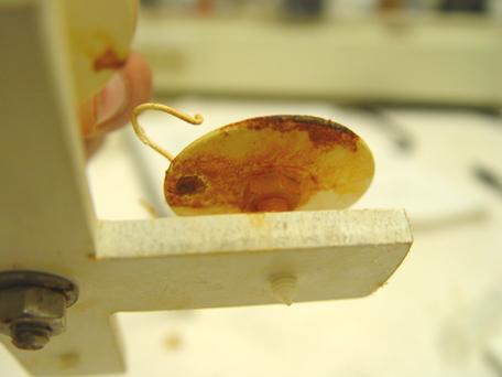
Figure 25. Photo. Bottom side of a sensor mounted on its holder experiencing under-paint corrosion.

Sensor Anode Fabrication

The same steels (lots) as the ones used for the chamber exposure were used to make the steel washers. They were machined using computerized numerical control (CNC) and then blasted using AC grade glass beads (60-120 U.S. screen, 0.124-0.25mm) to obtain a contaminant-free surface.

Sensor Cathode Fabrication

Previous studies showed that copper was a good compromise between cost and performance for the cathode even if gold was the best choice.(29,30) To be more cost effective, brass screws were copper- or gold-plated to make the cathodes.

Electrode Separator

Preliminary tests showed that nylon was a good choice for the separating material. It was neither too hydrophilic nor hydrophobic and provided a good surface tension to keep the water on its surface while still allowing the sensor to dry.

Sealer

Several sealing materials have been used in preliminary designs. A rubber adhesive was used to seal the different parts together and to impede the water from infiltrating between the parts.

Sensor Electrical Connection

Electrical connection was a special consideration. Classical soldering could not be used because of issues concerning the high temperature and the flux flow that would contaminate the steel surface. In addition, typical low temperature solders melt during powder coat curing which would damage the connection. After consideration of the constraints on this connection, the copper leads (14-gauge wires) were threaded, and the steel washer was tapped. Next, silver epoxy (conductive) was used as a thread locker to make sure the connection was established. The same connection was used for the copper lead on the central screw followed by an insulation overcoat (caulk). The electrical connections to the sensor lead wires were soldered and caulked with marine sealant to avoid the formation of a galvanic couple that might introduce errors.

Exposure Testing

To be consistent with task 2.1, the same exposure cycle (SAE J-2334) and exposure chamber were used for the sensor exposures so that corrosion values of the coupons could be compared with the coulomb values of the sensors. After the first set test, the most interesting environments were determined, and it was decided that the sensor would be exposed to six environments. Table 9 presents the compositions of the solutions used during this test. The sensors were given a 15-cycle exposure.

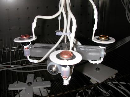
To hold the sensors horizontally, polyacrylate racks were custom made to fit in the exposure chamber. Figure 26 shows the setup for the sensors on the racks. A set of four different sensors (one of each type) was exposed per rack. Sensors were built following the construction matrix presented in table 10. Consequently, a total number of 24 sensors were built for the purpose of the exposure test.

The number preceding the sensor's name is the number of the solution used for the soaking (e.g., sensor 1-G-Q is an SAE1010 (Q) sensor with a gold (G) screw, and solution 3-1 (1) was used for the soaking).

TASK 2.3. DEVELOPMENT OF PROTOTYPE CABLE CORROSION SENSORS

Cable Sensors

Galvanic corrosion sensors were developed based on the steel and copper galvanic couple. The intent was to create a small sensor capable of insertion within the bridge suspension cable strands' parallel interstitial spaces. The sensor would respond to corrosive conditions producing a current proportional to the steel's corrosion rate in a wet or salt-laden environment within the cable. If the interior cable environment was dry, corrosion-inhibited, or protected by waterdisplacing compounds, no significant current would be expected from the sensor.

High-strength iron wire that had a diameter of 0.08 cm and a length of 3.5 cm acted as the anode. A copper wire with a diameter of 0.02 cm and a length of 20 cm was the cathode. The surface area ratio of Cu to Fe was approximately 1.4. An 11-MΩ resistor was soldered between the anode and cathode. The two lead wires were connected to the electrode ends opposite the resistor. Figure 27 and figure 28 show the parts used for the cable sensor and fabrication. The resistor and black lead wire were soldered to the iron anode, and the copper cathode was soldered to the red lead wire. The soldered areas were coated with epoxy and covered with shrinking olefin tube. The iron anode was cleaned using abrasive paper and methanol alcohol and then dried. After drying, porous fiberglass sleeving material was used to cover, or electrically insulate, the iron anode. The copper cathode was then wound around the sleeving material. A larger diameter fiberglass sleeve was placed over the anode-cathode assembly, and heat shrink tubes were installed at the sensor ends. The cable sensor was complete after the ends were sealed with marine-grade caulking. The response was tested by wetting it with 2 percent salt solution and allowing it to dry. Figure 29 shows the maximum current due to the corrosion of steel less than 100 µ A (design maximum). The fiberglass sleeving electrically insulated the anode and cathode from each other. It also insulated the sensor for the cable strands, but it allowed water, if present, to soak into the sensor.

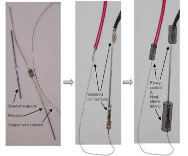
Figure 27. Photo. Components and fabrication of the cable sensor.

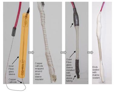
Figure 28. Photo. Completion of the cable sensor.

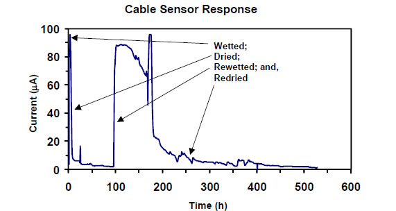
Figure 29. Graph. First test of corrosion sensor wetted, dried out, rewetted, and redried.

Cable Sensor Tests

A test specimen for the sensors consisted of 12 rods bundled with 3 sensors which had either loosely or well-sealed wrappings. Corrosion products were characterized and compared using XRD as in task 2.1. The anode and cathode surface areas were selected and tested to provide sensor output in the data logger's measurement range.

Figure 30 shows deployment locations within the multistrand cable specimen. Three tests were performed within a single multistrand specimen. A set of 18 tests were performed with the sensors (after single immersion in 1/10 Harrison solution) including drying, wet, and cycled exposures. Dilute Harrison solution consisted of 0.35 percent ammonium sulfate, (NH⁴)²SO⁴, and 0.05 percent NaCl. Table 11 provides the test matrix, which was modified to acquire additional data in some cases. The dry tests were soaked for 15 minutes in dilute Harrison solution then equilibrated (dried) on the laboratory bench top (50 percent relative humidity (RH)) while collecting data. The wet tests were soaked for 15 minutes in dilute Harrison solution and then equilibrated in a closed plastic container (100 percent RH) while collecting data. The cycled tests were not initially soaked before starting the cyclic test to observe the response to condensing humidity. They were then soaked for 15 minutes in dilute Harrison solution and returned to the cyclic chamber, and data were collected throughout the process.

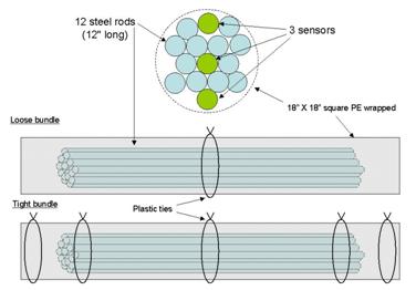
Figure 30. Illustration. Cable specimen showing arrangement of strands and sensors.

L = loose wrap.
T = tight wrap.
C = cyclic exposure.

XRD for Cable Sensor Tests

XRD was performed on corrosion products obtained from test specimen rods. The corrosion products on the sensor anodes were not expected to produce sufficient corrosion product to obtain useful results in each test.