U.S. Department of Transportation
Federal Highway Administration
1200 New Jersey Avenue, SE
Washington, DC 20590
202-366-4000
Federal Highway Administration Research and Technology
Coordinating, Developing, and Delivering Highway Transportation Innovations
 |
| This report is an archived publication and may contain dated technical, contact, and link information |
|
Publication Number: FHWA-RD-99-194
Date: June 2000 |
||||||||||||||||||||||||||||||||||||||||||||||||||||||||||||||||||||||||||||||||||||||||||||||||||||||||||||||||||||||||||||||||||||||||||||||||||||||||||||||||||||||||||||||||||||||||||||||||||||||||||||||||||||||||||||||||||||||||||||||||||||||||||||||||||||||||||||||||||||||||||||||||||||||||||||||||||||||||||||||||||||||||||||||||||||||||||||||||||||||||||||||||||||||||||||||||||||||||||||||||||||||||||||||||||||||||||||||||||||||||||||||||||||||||||||||||||||||||||||||||||||||||||||||||||||||||||||||||||||||||||||||||||||||||||||||||||||||||||||||||||||||||||||||||||||||||||||||||||||||||||||||||||||||||||||||||||||||||||||||||||||||||||||||||||||||||||||||||||||||||||||||||||||||||||||||||||||||||||||||||||||||||||||||||||||||
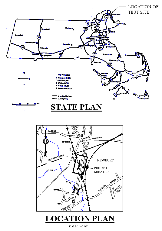
Development and Field Testing of Multiple Deployment Model Pile (MDMP)CHAPTER 5. MDMP TESTS AT THE NEWBURY, MA SITE5.1 Site Overview and LocationThe first field deployment of the MDMP was conducted at a site located in Newbury, MA during March 1996. Refer to Figure 34 for the site locus. The original construction of a multiple-span, reinforced-concrete bridge along Route 1 was completed in 1935. This bridge was demolished during the summer of 1996 and will be replaced by a new bridge currently being constructed at the site. The new bridge is being built to accommodate an extension of the Commuter Rail from Ipswich, MA and a new Commuter Rail station. The test location was chosen as the first test site for the MDMP because it contained a 9- to 12-m- (30- to 40- ft-) thick clay deposit close to the ground surface. This clay is ideal for assessing the pile capacity gain and pore pressure dissipation with time. In addition to the MDMP testing, full-scale instrumented piles will be tested at the site during future research phases. Both test and production piles for the new bridge will be conducted at the same location as well. This chapter provides information regarding the subsurface soils at the site, predicted MDMP behavior prior to installation, and a description of the testing procedure and schedule. The test results are presented in Chapter 6, with analyses in Chapter 7. 5.2 Previous Subsurface Exploration Program StudiesPrevious subsurface studies were conducted in the 1930's for the original bridge and again in 1988 and 1992 for the new bridge. Supplemental borings were performed in 1996 during the construction phase of the new replacement bridge. The 1930's study included six borings. A study for the initial evaluation for the foundation of the replacement bridge was completed in 1988. During this study, six borings were completed and eight undisturbed samples were collected and tested. Additional subsurface testing was conducted in 1992, including 20 borings and 8 test pits (GZA GeoEnvironmental, 1993). 5.3 UMass-Lowell Subsurface Exploration ProgramThe UMass-Lowell conducted several borings (designated as NB1, NB2, NB4, and B5) to determine the soil profile and properties within the immediate vicinity of the proposed model pile test location. The boring designation NB2 was also used for the first MDMP test. The boring designation NB3 was used for the second MDMP test at the same location as boring NB2. Figure 35 shows the location of the borings and the MDMP tests. A detailed subsurface investigation, with soil properties, will be presented by Chen (1997). The following sections outline the extent of the investigation and the major features related to the MDMP testing.
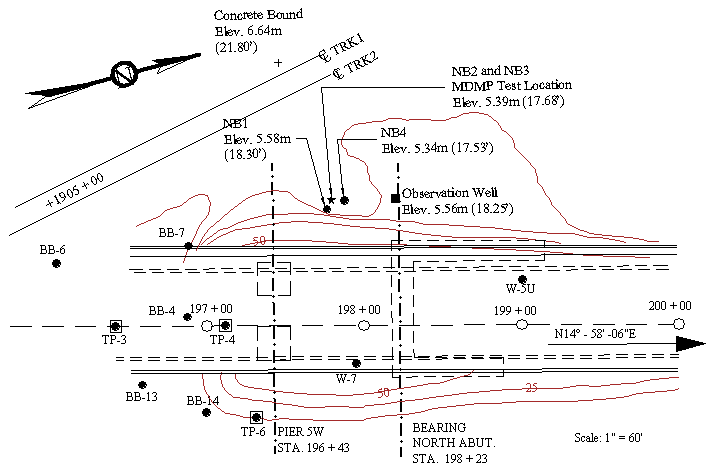
Figure 35. Newbury MDMP Site Plan. 5.3.1 Sampling and Field TestingTest boring NB1 was completed by New Hampshire Boring, Inc. of Londonderry, New Hampshire on September 25 and 26, 1995. The boring was conducted to evaluate the stratigraphy at the site and to obtain geotechnical properties of the clay deposit for correlations with the model pile tests. The boring was located approximately 12.2 m (40 ft) west of the existing northern bridge abutment in a position that will remain accessible after the completion of the entire project. The boring was initially advanced using a hollow-stem auger to a depth of approximately 3.05 m (10 ft) to the top of the clay. The auger was removed and 10.16-cm (4-in) I.D. casing was subsequently driven to a depth of 5.49 m (18 ft) below ground surface. The boring was then advanced using open-hole drilling techniques to the bottom of the clay layer at a depth of 16.46 m (54 ft) below ground surface. A 10.16-cm (4-in) I.D. casing was installed to stabilize the open hole as drilling continued until refusal was encountered at a depth of 31.09 m (102 ft) below ground surface. Split-spoon samples (S-1 through S-14) were taken at generally 1.52-m (5-ft) intervals within the fill layer and again within the stratified sand/silt/clay and till layers below the clay. Undisturbed tube sampling (T-1 through T-6) was performed within the clay deposit. In all, a total of 14 split-spoon and 5 undisturbed soil samples were successfully obtained. Table 16 provides a summary of the obtained samples with depth for NB1. Upon completion of the boring, an observation well was installed to a depth of 4.42 m (14.5 ft) below ground surface. Test boring NB4 was completed by New Hampshire Boring, Inc. from March 11 through March 18, 1996 during the MDMP testing program. This boring was necessary to determine the depth and quality of the bedrock, to install a piezometer, and to gather more undisturbed samples. The boring was initially advanced using a hollow-stem auger to a depth of approximately 3.05 m (10 ft), corresponding to the top of the clay. The auger was then removed and 10.16-cm (4-in) I.D. casing was subsequently driven to a depth of 4.27 m (14 ft) below ground surface. Wash and drive techniques were used to advance the boring to the top of the bedrock at a depth of 30.5 m (100 ft) below ground surface. Split-spoon samples (B-1, S-1 through S-15) were taken at generally 1.52-m (5-ft) intervals within the fill layer and again within the stratified sand/silt/clay and till layers below the clay. Undisturbed tube sampling (B-2, T-1 through T-3) was performed within the clay deposit. In all, a total of 15 split-spoon and 3 undisturbed soil samples were successfully obtained. Table 17 provides a summary of the obtained soil samples with depth for NB4. Upon the completion of the boring, a Vibrating Wire piezometer and an observation well were installed to a depth of 10.24 m (33.6 ft) and 7.92 m (26 ft) below ground surface, respectively. Test boring NB5 was completed by New Hampshire Boring, Inc., between September 3 and 4, 1996 in order to gather additional undisturbed samples in the clay layer. A 10.16-cm (4-in) I.D. casing was installed to 2.74 m (9 ft) below the ground surface. The boring was advanced using an open-hole drilling technique to a depth of 14.94 m (49 ft) below ground surface where casing was installed at the end of the first day. Undisturbed tube sampling (T-1 through T-6A) was performed within the clay deposit and interbedded sand/silt/clay deposit. In all, six undisturbed soil samples were successfully obtained. Table 18 provides a summary of the obtained soil samples with depth for NB5. Table 16. Sampling Performed at Boring NB1.
Table 17. Sampling Performed at Boring NB4.
Table 18. Sampling Performed at Boring NB5.
In addition, samples were recovered during the installation of the MDMP on March 6, 1996. Table 19 provides a summary of the obtained soil samples with depth for NB2. Table 19. Sampling Performed at Boring NB2.
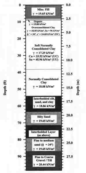
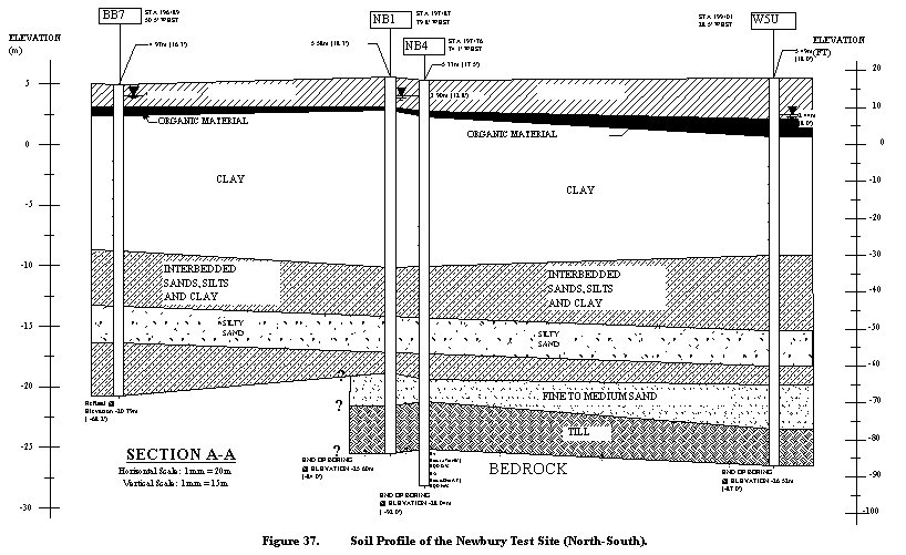
Standard penetration testing (SPT) was performed during split-spoon sampling to evaluate the resistance of the soil. SPT testing was conducted according to ASTM D 1586-84 using a 3.49-cm (1.375-in) I.D. split-spoon sampler typically driven 60.96 cm (24 in) with a 140-lb hammer falling from a height of 76.2 cm (30 in). Field strength index testing using the pocket penetrometer and the torvane devices were performed on selected split-spoon and undisturbed soil samples obtained from the clay layer. The pocket penetrometer is a device that provides a quick measure of the unconfined compressive strength of a clay by failing the clay in a "punching" mode under normal stresses. The unconfined compressive strength is theoretically twice the undrained shear strength. The torvane device provides a rough estimate of the undrained shear strength of a clay by failing the clay in a rotational "shearing" mode. In all, a total of six torvane and four pocket penetrometer tests were completed in the field. In addition, three field vane shear tests (FV-1 through FV-3) were performed in the upper portion of the clay stratum. 5.3.2 Groundwater MonitoringSeveral monitoring wells were observed by the UMass-Lowell to determine the groundwater elevation. An existing well with a 50.8-mm (2-in) PVC riser was located at the site (marked as"Observation Well" on Figure 35). This well was monitored until its apparent destruction during the construction of the replacement bridge. The monitoring well installed in NB1 was constructed with a 50.8-mm (2-in) PVC wellscreen attached to a solid PVC riser. The well is 4.42 m (14.5 ft) deep with a 3.05-m- (10-ft-) long PVC wellscreen, measured from the bottom upwards. The annular area above the screen between the well and the soil was sealed with bentonite. At NB4, a vibrating wire piezometer was installed to a depth of 10.24 m (33.6 ft) with approximately 0.305 m (1 ft) of sand placed above and below the piezometer. Bentonite pellets were used to seal the sand zone above and below the piezometer. The monitoring well in NB4 was installed to a depth of 7.92 m (26 ft) with 1.22 m (4 ft) of 50.8-mm- (2-in-) diameter PVC wellscreen and 6.71-m- (22-ft-) PVC riser. Bentonite pellets were used to seal above and below the wellscreen to ensure that the pore water pressure in the clay is measured. A roadbox set in cement was used as a cover to protect each well. The locations of the monitoring wells are shown in Figure 35. 5.4 Typical Subsurface StratigraphyFigure 36 presents the soil stratigraphy at the model pile test location. This stratigraphy is based on borings NB1, NB2, NB4, NB5, and other borings performed in the vicinity during previous subsurface studies. Figure 37 presents a soil profile based on four borings along the center line of the proposed construction. Referring to Figures 36 and 37, the general soil profile at the model pile test location (from ground surface downward) consists of the following soil strata: 2.44 m (8 ft) of granular fill composed of very dense, brown sand and gravel intermixed with frequent concrete fragments, overlying a thin layer (approximately 0.3 m (1 ft)) of highly compressible organic silt and peat. Below the fill and organics is an approximately 13.72-m- (45-ft-) thick deposit of a marine clay, known as Boston Blue Clay. The clay consists of approximately 2.74 m (9 ft) of medium stiff to very stiff, over-consolidated layer (crust), over 6.10 m (20 ft) of very soft to soft, plastic, normally to slightly over consolidated clay and 4.88 m (16 ft) of soft, plastic, normally consolidated clay. An interbedded deposit of silt, fine sand, and silty clay approximately 2.90 m (9.5 ft) thick underlies the clay. Below this interbedded deposit is a layer of silty sand approximately 2.44 m (8 ft) thick. Another interbedded deposit of silt, fine sand, and silty clay approximately 2.29 m (7.5 ft) thick underlies the silty sand. Below this interbedded deposit is a layer approximately 2.44 m (8 ft) thick of medium dense to dense, fine to medium sand. Underlying the fine to medium sand is a dense glacial till consisting of medium dense to dense, fine to coarse sand and gravel, with traces of silt and rock fragments. Based on the subsurface information within the vicinity of the model pile test location, mylonitic, basalt bedrock underlies the glacial till.
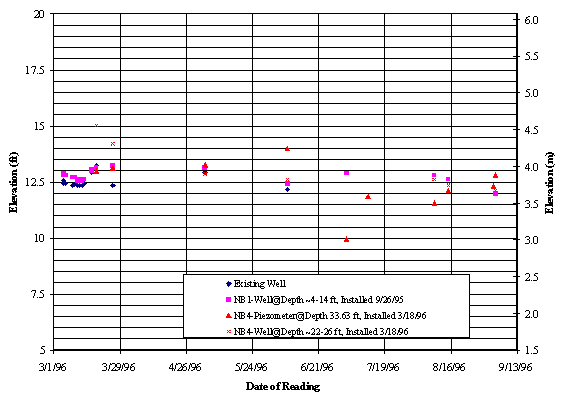
Figure 37. Soil Profile of the Newbury Test Site (North-South). Groundwater was periodically measured in the monitoring wells near the MDMP test area for the time period between March 5, 1996 and September 4, 1996. Additional measurements carried out at the site will be presented in subsequent reports. Based on these groundwater measurements, a relationship of groundwater elevation versus time is presented in Figure 38. Figure 38. Groundwater Elevations at the Newbury Test Site. 5.5 Engineering Properties of the Clay at the Newbury Test SiteLaboratory and field tests are being conducted and analyzed by Yu Lin Chen at the UMass-Lowell and will be presented in subsequent reports. The aim of this study is to determine the soil properties at the Newbury test site. Table 20 presents the preliminary test results of natural water content, Atterberg Limits, unit weight, shear strength based on various methods, sensitivity, and Over Consolidation Ratio (OCR) for the clay layers at the Newbury site. Figure 39 presents the profile of the maximum past pressure with depth in the clay layer. Figure 40 presents a profile of calculated and measured undrained shear strength with depth for the clay layer. The calculated values are based on preliminary results of Direct Simple Shear (DSS) tests that were performed on samples at depths of 9.37 m (30.75 ft) and 13.03 m (42.75 ft) by Don De Groot of UMass-Amherst. Based on the obtained test results, SHANSEP (Ladd and Foott, 1974) relationships were developed. For the sample at a depth of 9.37 m (30.75 ft), the recommended relationship is: Table 20. Summary of Soil Properties at the Newbury Site (based on the preliminary test results of Y.L. Chen).
Remarks: UU Test - Unconsolidated Undrained Triaxial Test
For the sample at a depth of 13.03 m (42.75 ft), the recommended relationship is:
In both cases, the DSS tests at the Newbury Site yielded lower strength parameters than the following typical relationship used for Boston Blue Clay (BBC): Using equation 5.1 as a representative relationship for the soft, normally consolidated clay layer (between depths of 5.49 m (18 ft) and 11.58 m (38 ft)) and equation 5.2 to represent the underlying normally consolidated layer (between depths of 11.58 m (38 ft) and 16.46 m (54 ft)) leads to the calculated undrained shear strength shown in Figure 40. These calculations make use of the OCR values presented in Figure 39. The calculated values in Figure 40 seem to compare well with the laboratory tests, suggesting that the DSS tests and SHANSEP relationship provide a reasonable description of the undrained shear strength of the clay layers at the Newbury test site. For the MDMP test NB2 that was conducted at a depth (to radial stress measurement) of 7.39 m (24.25 ft), the representative
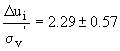
soil parameters are OCR 5.6 Predicted Behavior of the Multiple Deployment Model Pile5.6.1 OverviewThe MDMP's expected behavior was evaluated prior to deployment to determine the range of measurements and to develop a schedule of testing. This assessment "prediction" was based on the findings and methodology presented in an earlier phase of the time-dependent pile capacity research (Paikowsky et al., 1995). The present section provides the details of this evaluation as it pertains to the magnitude of excess pore pressure, time and dissipation rate of the excess pore pressure, and capacity gain rate and time. 5.6.2 Estimated Increase in Pore Water Pressure Due to DrivingFigure 41 presents the initial excess pore pressure distribution for clays with an OCR range of 1 to 10 and pore measurement at a distance of 17 radii or more from the pile tip (representing the "shaft" condition along the pile). The data in Figure 41 suggests that the ratio of average initial excess pore pressure to vertical effective stress for a large variety of clays (79 cases) can be estimated to be:
Figure 41. Initial Excess Pore Pressure Distribution
(only readings for 1<OCR<10 included) (Paikowsky et al., 1995).
The effect of OCR on the ratio of initial excess pressure can be estimated through the relationship presented in Figure 42. Based on the MDMP installation depths to the pressure transducer and total pressure
cell of 7.39 and 10.45 m (24.25 and 34.30 ft), the total and hydrostatic
pressures at these depths are 146.85 and 205.21 kPa (21.30 and 29.76 psi) and
57.02 and 87.43 kPa (8.27 and 12.68 psi), respectively. These values lead to a vertical effective
stress of 89.83 and 117.78 kPa (13.03 and 17.08 psi) for depth to pressure
instruments of 7.39 and 10.45 m (24.25 and 34.30 ft), respectively. Considering equation 5.4, the expected magnitude of the initial pore pressure is 205.71 and 269.72 kPa (29.83 and
39.12 psi). Based on laboratory tests and equation 5.5, the soil at a depth of 7.39 m (24.25 ft) has an OCR 5.6.3 Estimated Time for Excess Pore Water Pressure DissipationThe MDMP is designed to capture the pore pressure increase due to penetration and the subsequent dissipation of the excess pore pressures. From the data compiled and analyzed by Paikowsky et al., 1995, the rate of pore pressure dissipation can be used to estimate the time required for the excess pore pressure to dissipate. The method presents normalized excess pore pressure relative to the initial excess pore pressure after penetration. When plotted on a semi-log plot, the best fit line from 20% to 80% dissipation represents the linear portion of the curve. The equation of the line is: where:
Hut = horizontal pore pressure dissipation parameter t = time after pile driving (seconds) Utilizing data from the test in Boston Blue Clay, the horizontal pore pressure dissipation parameter, Hut, is 0.498±0.067. To reference the rate to time scale, the time at 50% dissipation, t50, for BBC is 1.57 h ±0.334 h. This data was normalized to a pile with a radius of the PLS cell (equal to 19.177 mm). To correct the time of 50% dissipation to the size of the MDMP with a radius of 38.1 mm, the following equation is used:
Figure 42. Effects of OCR on u/
where: t1 = elapsed time since driving adjusted to a standardized pile size t2 = actual time since driving for a known pile r1 = radius of standardized pile r2 = radius of a known pile Substituting the geometrical relationships of the PLS cell and the MDMP into equation 5.7 leads to:
The adjusted time to 50% dissipation of the excess pore pressure around the MDMP is therefore t50 = 6.21±1.32 h. Using the range of t50 and the average dissipation rate of Hut = 0.498 leads to the estimated range of dissipation time presented in Figure 43. According to the obtained relations, 80% of the excess pore pressure will dissipate after about 25 h, with a possible range (based on 1 S.D.) between 18 and 35 h. 5.6.4 Estimated Time for Capacity GainIn order to assess the rate of capacity gain, Paikowsky et al. (1995) obtained the relationship between the ratio of the pile capacity to the maximum capacity over time. These relationships allow the prediction of the pile capacity gain with time using a process similar to that used for the prediction of the pore pressure dissipation with time. The estimation of the time required for the MDMP capacity gain is based on the following relationship between the rate of gain and the normalized capacity:
where: Rs(t) = pile shaft capacity at any time "t" after driving Rs max = maximum pile shaft capacity Cgt = parameter representing the rate at which the pile gains capacity t = time after pile driving (hours) The data on which Cgt is based requires the measurement of capacity with time after driving, which is difficult to obtain. The correct relationship of equation 5.9 should be based on the skin friction at a zone along the pile for which the assumption of radial consolidation is valid. While these values are measured by the MDMP, they were not readily available for many cases. Therefore, the Cgt parameter evaluation was carried out in the following ways: (1) Based on data related to the total pile capacity: Cgt = 0.389±0.119 (1 S.D.) (for 15 cases). (2) Based on data related to the friction along the pile: Cgt = 0.356±0.088 (1 S.D.) (for 17 cases).
The values used for evaluation of the MDMP are based on the average from all data where Cgt = 0.367±0.096 (for 39 cases). In order to align the dissipation rate to a specific time, the time to 75% capacity gain was used by Paikowsky et al. (1995). This time was found to be: (1) Based on data related to the total pile capacity: t75 = 385.0±226.3 h (1 S.D.) (for five cases). (2) Based on data related to the friction along the pile: t75 = 539.5±336.2 h (1 S.D.) (for 12 cases). The values used for evaluation of the MDMP are based on the data when measurements of friction along the shaft of the pile were analyzed, where t75 = 539.5±336.2 h (for 12 cases). These times are all related to a 30.48-cm- (12-in-) diameter pile. Equation 5.7 can be used to adjust t75 to the MDMP size as shown in equation 5.10:
The resulting value of t75 = 33.7±21.0 (1 S.D.) hs was used to develop Figure 43. The relationship shown in Figure 43 is based on Cgt = 0.356 and t75 = 33.7±21.0 h (1 S.D.). This suggests that 80% of the MDMP maximum frictional capacity will be obtained about 47 h after driving, with a possible range of 17.6 to 75.6 h. 5.7 MDMP Testing Procedure5.7.1 OverviewThe MDMP testing program was conducted during March 1996. The tests were conducted at the locations marked as NB2 and NB3 (adjacent to the location of boring NB1) as shown in Figure 35. The drilling, installation, and removal of the MDMP were carried out with the assistance of New Hampshire Boring, Inc., of Londonderry, New Hampshire. Personnel
and Data Acquisition Systems were housed in a tent supplied by the Army
Research Labs in Natick, MA. A kerosene
heater was used to keep the equipment above freezing temperatures. Power was supplied via two portable
generators. Major weather variations
took place during the testing, including 0.61 m (2 ft) of snow in the first
week of testing, followed by rapid snow melt.
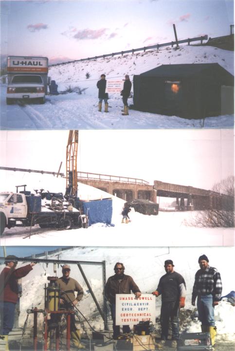
Figure 44 presents three photographs depicting the general layout of the
site. Figure 44a shows the site as
equipment was delivered and the DAS was assembled in the tent. Figure 44b was taken during a snowstorm while
the drill rig was in place over NB4.
The blue structure attached to the drill rig was temporary protection
around the static load frame during MDMP test NB2. Figure 44c shows the static load frame with the independent
reference beam.
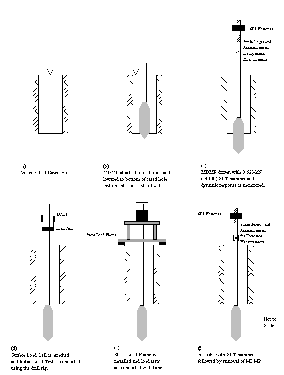
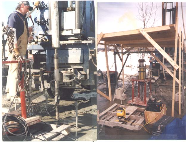
The purpose of the testing program was to measure the excess pore pressure dissipation, the gain of capacity with time, and soil and pile responses during installation and removal. The tests at the Newbury site were conducted in the soft to medium normally consolidated clay, representing easy driving conditions. Although the MDMP was designed to be advanced to any desired depth using drill rods, the test hole was cased to the bottom of the drill rods, ensuring that soil friction did not develop along the rods. Figure 45 shows the steps of a typical MDMP installation and testing performed at the Newbury site. 5.7.2 General Test PlanThe first step involved drilling a vertical 10.16-cm- (4-in-) diameter cased hole through the fill region to approximately 3.05 m (10 ft) below the ground surface. Next, four helix anchors for the static load test frame were installed. Due to existing concrete outwash in the fill, it was necessary to pre-auger holes, place the four anchors, and then backfill with ready-mix concrete to secure the anchors. Drilling was then continued through the stiff upper clay. Split-spoon samples were gathered in the stiff clay as drilling proceeded to determine the transition zone from the stiff yellow desiccated overconsolidated clay to the soft to medium blue clay. The transition was identified approximately 5.49 m (18 ft) below the ground surface. The casing was then driven and washed out to a depth of 6.25 m (20.5 ft) below the ground surface. The 61-m (200-ft) instrumentation cable was threaded through the drill rods. The rods were attached to the MDMP and lowered into the cased hole. The top of the drill rod was instrumented with strain gauges and accelerometers as part of the dynamic measurements. The borehole was completely filled with water and the MDMP was held in place in order to stabilize the temperature of the instrumentation and check the data acquisition system. The MDMP was then driven with a 0.623-kN (140-lb) safety hammer (see Figure 46a). The PDA was used to measure the force and velocity in the rods at the surface and inside the MDMP during driving. The initial hammer stroke was 15.2 cm (6 in) and was increased to 30.5 cm (12 in) and then again to 45.7 cm (18 in) after inspection of the stresses measured by the PDA. The driving stresses were kept between approximately 138 and 207 MPa (20 and 30 ksi) to avoid damage to the MDMP sensors. Driving continued until the entire instrumented section of the MDMP was driven deep enough into the clay and the top of the drill rods reached the level required to attach the pile to the static load frame. Monitoring of the MDMP during driving was accomplished with an additional Pile-Driving Analyzer on loan from the Federal Highway Administration. A 222.4-kN (50,000-lb) load cell was attached between the drill rod string and the drill rig connection. Two displacement transducers were fixed to a reference beam and positioned to measure the vertical movement at the top of the drill rod string. The initial static load test was completed with the drill rig applying the loading force at a slow rate.
Figure 45. Steps for Installation and Testing of the MDMP at the Newbury Site. The assembled static load frame was lifted in place, screwed to the anchors, and attached to the MDMP (see Figures 46a and b). Several static load tests were conducted with increasing time intervals between tests. Each load test was performed in tension at a near constant load rate for a predetermined amount of displacement (usually 12.5 mm). The intervals between static load tests were determined as the test progressed to assess the gain of capacity with pore pressure dissipation. A final load test was performed when the excess pore pressure due to installation had dissipated. The final load test consisted of a series of rapid cyclic loading and unloading cycles to determine the pile capacity independent of the strain rate. Before the removal of the MDMP, the pile was driven again (restrike) and dynamic measurements were recorded with two PDAs. For both MDMP tests NB2 and NB3, measurements of force, displacement, total lateral pressure, and pore pressure were recorded continuously by the HP DAS after the pile had been successfully driven. During driving and restrikes, two PDAs were used to monitor the three internal load cells and accelerometers, and the additional strain gauges and accelerometers at the top of the drill rods. The total lateral pressure and pore pressure were also recorded by the HP DAS during driving and restrikes. 5.7.3 Testing Procedure for the MDMP during Test NB2On March 6, 1996, the first of two model pile tests was conducted at the Newbury site. A borehole was washed and cased to a depth of 6.25 m (20.5 ft) below ground surface. The MDMP was inserted into the cased hole and came to rest so that the tip was 6.50 m (21.34 ft) below the ground surface. The PDA gauges were attached and the MDMP was allowed to stabilize for 1 h and 5 min. A safety hammer was used to install the MDMP with an increasing stroke of 15.2, 30.5, and 45.7 cm (6, 12, and 18 in). During driving, the pile penetrated a total of 2.57 m (8.42 ft) in 8.78 min. The initial load test using the drill rig started at 25.23 min after the start of driving. The pile was pushed 53.1 mm (2.09 in) to ensure that the slip joint was completely closed, and then pulled in two steps for a total 133.9 mm (5.27 in) until the slip joint was completely open. At the end of the tension load test, the slip joint immediately collapsed under the self-weight of the pile when the pile was disconnected from the drill rig. Forty minutes after the start of driving, the MDMP was pushed approximately 15.2 cm (6 in) to allow proper attachment with the hydraulic ram and static load frame. At this point, the static load frame was moved into place and the pile was connected. During the connection process, some unrecorded displacement may have taken place. Once the static load frame was properly attached, the MDMP tip was at a depth of 9.31 m (30.56 ft) below ground surface. For approximately the next 6 days, the MDMP was continuously monitored using the HP DAS. Eleven static tension load tests were performed using the static load frame. Table 21 shows the time, displacement, and rate of movement for all tests. Following load test #11, the final load test was performed 137.7 h after the start of installation. The final load test consisted of a series of alternating compression tests to failure, followed by tension tests to decrease the load at the top of the pile to approximately zero. Table 22 shows the time, duration, delay between each movement, displacement, and average displacement rate of all of the tests in the final load test sequence. Table 21. The MDMP Static Load Tests During Test NB2.
Table 22. The MDMP Final Loading Sequence During Test NB2.
Following the final sequence of static load tests, a restrike test was performed. The pile was driven 40.64 cm (16 in) using a 45.7-cm (18-in) stroke. The pile was then removed from the borehole utilizing the safety hammer to "bump up" the MDMP and drill rods to break soil resistance. A cake of clay was observed around the pile equal to the I.D. of the casing. When the clay cake was removed, the porous stones were missing. However, the soil did not appear to have entered the ducts that connect the porous stone cavity to the pressure transducer. During the installation of the pile, damage occurred to the load cell at the tip of the MDMP. This was evident by the increasing load measured during the entire time the pile was in place. After examining the load cell, one of the strain gauges was found to be damaged. The total pressure cell was also damaged at some point during the test, most likely during the removal of the MDMP. 5.7.4 Testing Procedure for the MDMP During Test NB3On March 13, 1996, the second of the two model pile tests was conducted at the Newbury Site. The same borehole used in the first test was washed and cased to a depth of 9.30 m (30.5 ft) below ground surface. The MDMP was inserted into the cased hole with its tip resting at 9.58 m (31.42 ft) below the ground surface. The PDA gauges were attached and the MDMP was allowed to stabilize for 1 h and 42 min. A safety hammer was used to install the MDMP using a stroke of 45.7 cm (18 in). During driving, the pile penetrated a total of 2.23 m (7.33 ft) in 5 min. Six additional blows were required to set the pile to the final depth for attachment to the static load frame. The initial load test, utilizing the drill rig, started 21.52 min after the start of driving. The pile was pushed 97.5 mm (3.84 in) to ensure that the slip joint was completely closed. At this point, the static load frame was installed and the pile was connected to the hydraulic ram. The connection process was changed to limit displacement that occurred during the first testing sequence. The new connection procedure involved attaching the loading rod to the drill rod string and then moving the ram up enough to bolt the loading rod to the ram. Unfortunately, there was slack between the loading rod and the hydraulic ram because of problems encountered in leveling the static load frame. This may have caused the erroneous displacement measurement observed during load test #1. Another factor that may have affected this reading is that the two DCDTs at the pile head may not have been properly secured to the reference beam. After load test #1 was completed, the MDMP tip was at a depth of 12.3 m (40.42 ft) below ground surface. For approximately the next 5 days, the MDMP was continuously monitored using the HP DAS. Nine static tension load tests were performed using the static load frame. Table 23 shows the time, displacement, and rate of movement for all nine static load tests. Following load test #9, the final load test was performed 119.4 h after the start of installation. The final load test consisted of a series of alternating compression tests to failure, followed by tension tests to decrease the load at the top of the pile to approximately zero. Table 24 shows the time, duration, delay between each movement, displacement, and average displacement rate of all of the tests in the final load test sequence. After the entire sequence of static load tests, a restrike test was performed on the MDMP with the 0.623-kN (140-lb) safety hammer. The pile was driven 1.22 m (4 ft) using a 45.7-cm (18-in) stroke. The pile was then removed from the borehole utilizing the safety hammer to "bump up" the MDMP and drill rods to break soil resistance. A cake of clay was observed around the pile equal to the I.D. of the casing. The porous stones did not fall out this time since thicker stones (10.2 mm) were used during the second test. The stones were approximately 5.1 mm thick in the first test. The lower load cell and total pressure cell did not function properly during any part of the second test. Table 23. The MDMP Static Load Tests During Test NB3.
Table 24. The MDMP Final Loading Sequence During Test NB3.
Ladd and Foott, 1974, "New Design Procedure for Stability of Soft Clays," ASCE Journal of Geotechnical Engineering Division, July.
|
||||||||||||||||||||||||||||||||||||||||||||||||||||||||||||||||||||||||||||||||||||||||||||||||||||||||||||||||||||||||||||||||||||||||||||||||||||||||||||||||||||||||||||||||||||||||||||||||||||||||||||||||||||||||||||||||||||||||||||||||||||||||||||||||||||||||||||||||||||||||||||||||||||||||||||||||||||||||||||||||||||||||||||||||||||||||||||||||||||||||||||||||||||||||||||||||||||||||||||||||||||||||||||||||||||||||||||||||||||||||||||||||||||||||||||||||||||||||||||||||||||||||||||||||||||||||||||||||||||||||||||||||||||||||||||||||||||||||||||||||||||||||||||||||||||||||||||||||||||||||||||||||||||||||||||||||||||||||||||||||||||||||||||||||||||||||||||||||||||||||||||||||||||||||||||||||||||||||||||||||||||||||||||||||||||||


 (5.1)
(5.1) (5.2)
(5.2)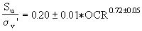 (5.3)
(5.3)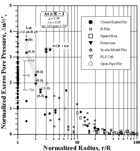
 (1 S.D.) (5.4)
 (5.5)
(5.5) (5.6)
(5.6)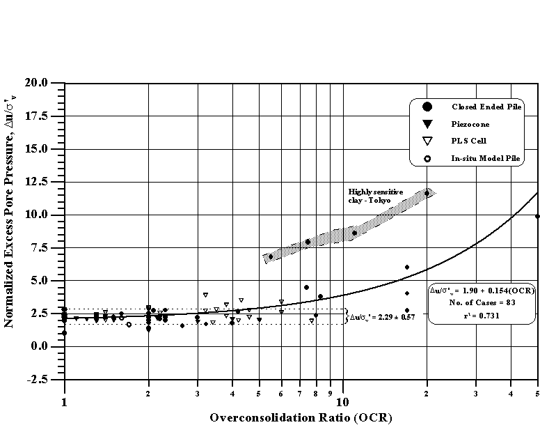
 (5.7)
(5.7)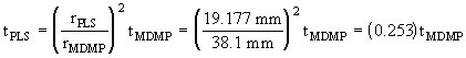 (5.8)
(5.8) (5.9)
(5.9)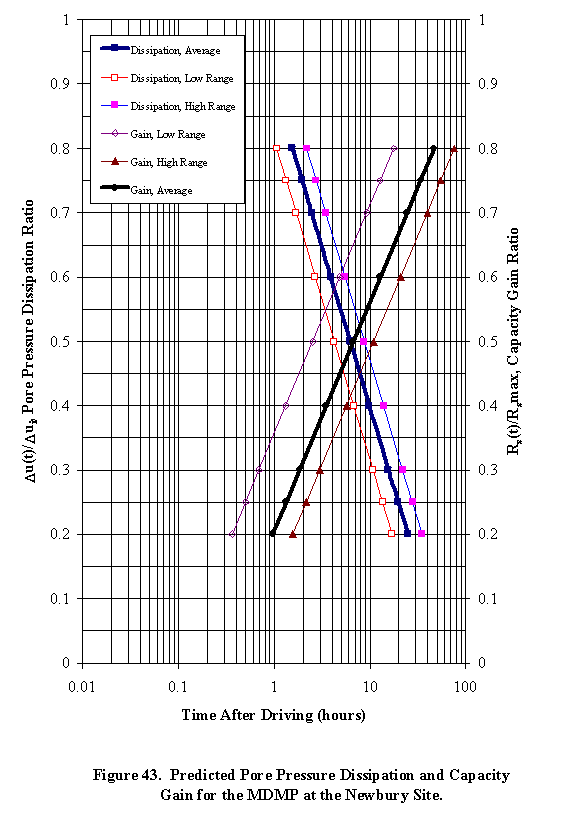
 (5.10)