Detection Technology for IVHS
2. Synopsis of the Final Report
The Task L Final Report contains a summary of the types and accuracies of traffic data that may be useful for several IVHS traffic management strategies, the planning that went into the execution of the project, and the data and conclusions from the Detection Technology for IVHS project that ran from September 1991 through April 1995. This section presents a summary of the findings from the Final Report. The complete Table of Contents from the Task L Final Report is included in Appendix A to provide more comprehensive information about the contents of the report.
2.1 ABSTRACT
As part of the U.S. FHWA-sponsored Detection Technology for IVHS program, ultrasonic, microwave radar, infrared laser radar, nonimaging passive infrared, video image processing with visible and infrared spectrum imagery, acoustic array, high sampling rate inductive loop, conventional inductive loop, microloop, and magnetometer detector technologies were evaluated at freeway and surface street arterial sites in Minnesota, Florida, and Arizona. These states were chosen because they exhibited a wide range of climatic conditions. The criteria for selecting the detector evaluation sites included searching for roadways with high traffic density and suitable structures for mounting the overhead detectors. Approximately 5.9 Gbytes of digital and analog vehicle detection and signature data and more than three hundred video tapes of the corresponding traffic flow were recorded. The detector outputs were time tagged and recorded on 88 Mbyte magnetic cartridges by using a data logger specifically designed and built for this project. Data analysis software was written to convert the raw data into an easily accessible Paradox database format compatible with a Windows personal computer operating system. Traffic volume ground truth data, obtained by counting vehicles from the recorded video imagery, were compared with the counts from the detector outputs. Speed ground truth data, obtained by driving probe vehicles through the field of view of the detectors and noting the vehicle speed as measured by the vehicle instrumentation, were compared with the speed measurement from the detectors. Several types of detectors were
found to satisfy current traffic management functions. However, improved accuracies and new types of information may be required from detectors for future traffic management applications.
2.2 TRAFFIC PARAMETERS
Flow rate, speed, and density (or its surrogate occupancy) are interrelated and together describe the quality of traffic flow on a highway.1 To measure flow rate accurately, detectors need to discriminate between vehicles traveling with spatial gaps on the order of one to two car lengths and average time headways of about 1.5 to 2 seconds, although headways of 0.5 second are not uncommon in congested areas. Speeds have been measured in the past with speed traps composed of two closely spaced (ten to twenty feet apart) inductive loop detectors; a
single detector with multizone capability that makes use of time of passage information; or with microwave radar, laser radar, or ultrasonic detectors that exploit the Doppler effect. Density (vehicles per mile per lane) is difficult to measure directly, except with some type of picture format such as video imaging or aerial photography, although indirect measurement is possible by dividing measured traffic flow (vehicles per hour per lane) by speed (miles per hour). Consequently, lane occupancy (the percent of time the detection zone of a detector is occu-pied by a vehicle) is often used as a surrogate measure for density. To accurately measure occupancy, the time that vehicles are within a detector’s sensing area must often be known to within 1 to 5 percent of its true value.
Other traffic management parameters of importance include presence, queue length, travel time, intersection turning movements, and vehicle classification. Presence needs to be measured, even if the vehicle is stopped, for signal activation applications. Therefore, detectors that require motion to be activated, e.g., Doppler-type microwave detectors, magnetic detectors, and some infrared, cannot perform this task.
Queue length requires wide area detection to be measured directly, as does density. Point detectors that measure presence at specific distances from a stop line can be used to estimate queue length. Travel time is inversely proportional to average speed. However, for travel time to be measured directly, a network-wide interrogation system is needed. Thus, travel time could be a side benefit of instituting an automatic vehicle identification (AVI) system in which the vehicles act as "probes". However, AVI systems are beyond the scope of the field test portion of this project. Imaging systems, high resolution ranging systems such as laser radars and some ultrasonic systems, and inductive loop detectors (ILDs) coupled with special vehicle transmitters and receivers also have the ability to classify vehicles.
2.3 SAMPLE TRAFFIC PARAMETER SPECIFICATIONS FOR IVHS
Guidelines were developed to assist the reader in defining the traffic measurement needs and detector performance requirements for representative IVHS services. However, no claim is made as to the widespread applicability of the specifications since they will necessarily vary with the selected IVHS architecture, implementation strategies, selected components and signal processing algorithms, and system operational procedures.
The traffic parameter specifications for a given management strategy must primarily take into account the data processing and traffic control algorithms for which these parameters serve as inputs. Specification of traffic parameter accuracy, therefore, cannot be separated from the overall system level analysis and design process. For each contemplated IVHS service, there are likely to be many different system algorithms, procedures, and detection subsystem design options. Evaluating the alternative implementation for a particular service is the responsibility of system analysts and designers. This report cannot serve as a substitute for a thorough systems analysis and design effort. Nonetheless, a process is suggested for the development of traffic parameter specifications that include data types, collection interval, and accuracy.
To structure the discussion and presentation of detector performance specifications, three general categories of traffic parameters are defined based on their intended use and the required timeliness of their input for the real-time traffic management strategy. These categories are tactical, strategic and historic. While the same raw inputs may often feed each of the categories, each presents a somewhat different set of detection perform-ance and sampling requirements. In fact, these differences can result in a detector technology or product being adequate for some applications and not for others.
The traffic parameter input ranges and accuracies identified are for some of the more common IVHS services that include signalized intersection control, freeway incident management, and freeway metering control. The parameters are categorized as either tactical, strategic, or historic. Range and accuracy values are derived or inferred from the accuracy needed for use in a particular algorithm (when it is known) and from practical experience with operating systems. Many of the historic and strategic category parameters may also be applicable to a host of other static and dynamic trip/route planning-related IVHS services. However, for these and other services where established strategies and algorithms are less common, a system-specific parameter requirements analysis effort is suggested. Such analysis is beyond the scope of this study.
To a large extent, current traffic management systems are input constrained. That is, a complete microscopic (vehicle-by-vehicle) view of the traffic stream is not available in today’s systems because of the lack of applicable real-time input data, even though the accelerating advances in computer processing and distributed system designs make possible advanced traffic optimization modeling and control in near real time. In this case, current systems rely heavily on prestored turning movement and origin-destination (O-D) data to supplement incomplete real-time data. In real-time control, the analysis and response to external events are performed and determined within specified time limits, usually of the order of seconds or milliseconds. In near real-time control, the feedback response is calculated within longer time intervals that are not small enough to respond to the stimuli in real time, but are sufficiently small to still have a positive impact on the events caused by the stimuli.
It is difficult to calculate the accuracy re-quired of traffic parameters for applications where algorithms do not exist or where improved algorithms are being sought. Future applications will not likely require a whole new set of traffic parameters. Rather, advanced detector technologies will provide greater area coverage with better vehicle characterization (e.g., presence, speed, classification, and turning movements), increased reliability, and reduced costs. Advanced control systems with vehicle tracking capabilities are also being developed and tested. These technology trends will be key enabling factors in the widespread deployment of advanced control algorithms that may include neural networks and expert system techniques. The net result will be an increased emphasis on tactical-type inputs and on requirements for increased accuracy and precision.
Figure 1 shows a formal process for development of traffic detector specifications. The first phase requires a detailed up-front systems analysis to properly specify all the subsystems that are part of the traffic management system architecture. Among these is the detection subsystem highlighted in the figure. The critical first step in defining traffic parameter specifications, such as signal processing algorithms, types of output data (count, speed, occupancy, etc.), parameter accuracies, data collection interval, and spatial resolution, is the identification of the overall system requirements, shown as inputs to the systems analysis process. These are normally based on a higher level evaluation of system goals and objectives [L.A. Klein et al., 1993].2
2.3.1 Detector Specification Development
Figure 1 shows a formal process for development of traffic detector specifications. The first phase requires a detailed up-front systems analysis to properly specify all the subsystems that are part of the traffic management system architecture. Among these is the detection subsystem highlighted in the figure. The critical
first step in defining traffic parameter specifications, such as signal processing algorithms, types of output data (count, speed, occupancy, etc.), parameter accuracies, data collection interval, and spatial resolution, is the identification of the overall system requirements, shown as inputs to the systems analysis process. These are normally based on a higher level evaluation of system goals and objectives [L.A. Klein et al., 1993].2
To meet the requirements for a particular traffic management application, a number of subsystem architectures, algorithms, and traffic parameters can be selected to function either singularly, or in combination with one another. The alternatives must then be analyzed and their performance compared with the overall system goals and objectives. The analysis of the alternatives not only requires a knowledge of the basic system requirements, but also a detailed under-standing of the system’s targeted operating environment and the constraints imposed by the available technologies that are a part of the solution. Knowledge of key technical specialty areas is needed so that they may be applied effectively in the development and implementation of IVHS architectures. These specialties include traffic surveillance and control algorithm design, traffic flow theory, statistics and sampling theory, computer technology, communications technology, and detector technology.
Once the systems analysis phase is complete, the detection subsystem design phase can begin. The major components of this phase are location of the detector stations, selection of detector technologies (there may be more than one), definition of station configurations, and definition of detector specifications.
2.3.2 Traffic Parameter Categories
The definition of traffic parameter specifications for IVHS used here takes into account three categories of parameters: tactical, strategic, and historic. Each suggests different usage of the data by a traffic management application that, in turn, generally dictates a different set of parameter specifications including data collection interval, range, and accuracy.
2.3.2.1 Tactical Input Parameters
Tactical parameters are those utilized in tactical decision making. Tactical decisions are defined as the expedient decisions made by a control system in response to real-time traffic parameter inputs. Tactical decisions are typically based on rote logic embedded in a predefined algorithm. One example is the real-time adjustment of a traffic-adaptive controlled signalized intersection in response to the measured cyclic traffic flow profiles on each approach. Another example is the decision to declare a freeway "incident" condition in response to a mainline lane parameter value exceeding a prescribed threshold.
Figure 1. Detector specification process
Because tactical decisions are made in quick response to changing real-time traffic variables, tactical parameters are generally collected over short time intervals (usually of the order of a few seconds). They may also be event driven, as for example a vehicle detected by a presence detector. Since tactical parameters
are collected on these shorter intervals, fewer vehicles are included in each sample. Variation from sample to sample will be exhibited due to the random nature of vehicle arrivals. The limited sample size will usually impose increased accuracy and precision on the measurement of tactical parameters. For example, the measurement of approach speed as an estimate of travel time for vehicles approaching a signalized intersection requires increased accuracy and precision when traffic signal offset decisions are being made, as compared to measuring average approach speeds for strategic background "plan-based" decision making.
2.3.2.2 Strategic Input Parameters
Strategic input parameters support strategic level decisions. These traffic control and management decisions generally operate at a higher level in the system hierarchy than do tactical decisions. Strategic decisions are typified by the activation of a preplanned management strategy in response to broad indicators of traffic flow conditions.
Strategic level decisions are often broader in geographic scope than tactical ones and often change the mode of an entire system or a large subsystem. Strategic decisions can be expert system rule-based, as in the Los Angeles Smart Corridor Management System, or algorithm-based, as used in Urban Traffic Control System (UTCS) plan selection. They frequently employ predefined scenarios and operator confirmation and approval processes.
Strategic traffic parameters are usually collected over a period of minutes rather than seconds; as a result, samples are larger. Most currently deployed freeway management and centralized traffic signal control systems use running averages and other filtering techniques to smooth out short term variations in the traffic stream data. Strategic traffic parameters are often input to maintain online data bases of current traffic conditions used by the management systems.
One example of a strategic level decision process is the selection of an incident management plan in response to a detected incident on a surface street network. When an incident condition is declared, the strategic decision process might monitor overall network conditions and implement an appropriate control plan overriding or adjusting the tactical level decision making process.
2.3.2.3 Historic Input Parameters
Historic input parameters are those used to maintain or update online historic traffic databases. These databases typically include traffic data collected over periods of five minutes or greater and are archived by time of day and day of week or by time of day and date. The primary purpose of historic data-bases is to provide information for offline planning and design operations. However, historic data are also commonly used as inputs to online tactical and strategic decision processes. For example, most freeway management systems maintain a file of historic flow rate data. This file is regularly used online as input for predicting future near-term traffic demands. In addition, some UTCS applications use historic flow rate data as input to online detector failure monitoring logic.
2.3.3 Matching Traffic Parameter Needs to Selected IVHS Services
As previously discussed, individual traffic parameters and accuracies required for a given application are specified by the algorithms, strategies, and operating procedures used to implement that application. A list of criteria which can help select traffic parameters for use in a particular IVHS application include:
- Convenience of parameter measurement;
- Amenability of resultant data to real-time processing;
- Existence of significant differences in parameter values within the range of traffic conditions that must be monitored.
Traffic parameter range, collection interval, and accuracy for application to signalized intersection control, freeway incident management, and freeway metering are presented in Tables 1 to 3. Unfortunately, the search of the available literature uncovered little universally applicable information regarding the required accuracy of traffic parameters for these or other services. Consequently the specifications presented are based on: (1) the data that were located, (2) operating experience, and (3) sensitivity analyses developed during the study
or found in the literature. The estimates are considered representative of those for the selected traffic parameters and are consistent with the general requirements of the particular application. However, for those parameter specifications applicable to a specific system design or to services not covered, a detailed analysis
is recommended. Such analyses are outside the scope of this study.
2.3.3.1 Signalized Intersection Control
Table 1 gives selected traffic parameter specifications for advanced signalized intersection control applications. Parameters are listed for the tactical, strategic, and historic categories. Tactical parameters include those relating to flow, speed, and occupancy measurements. For advanced signal control systems, typical flow-related parameters may include cyclically collected intersection approach flow rates, flow profile data, and turning volumes.
Tactical information related to intersection control is often collected on a cyclic basis and normalized to hourly rates. This minimizes the short term parameter fluctuations caused by data collection intervals being inconsistent with whole multiples of the cycle length. This problem can also be resolved by maintaining weighted running averages and by various other smoothing techniques [A. Gelb, 1980].3
Speed-based parameters are also of benefit to advanced signal control algorithms. In a tactical sense, vehicle approach speeds can be used to estimate link travel time. However, the accuracy of the speed measurement is critical in this case because a small error can have a significant effect on calculated travel time.
(This depends, of course, on the length of the approach section.) An error in calculated travel time of only a few seconds can have an adverse effect on operations if travel time is used as the basis for offset calculations. Another useful speed measure is the distribution of approaching vehicle speeds. The standard deviation of the measured speed can serve as an important input to the modeling of platoon dispersion from one signalized intersection to another.
Occupancy-based measures such as queue length, delay, and percent of stops collected on a cycle basis can also be tactical inputs to advanced signal control algorithms. Data from traditional inductive loop traffic detectors on an approach to a signalized intersection provide estimates for these parameters using an input-output model which also receives the current green state of the traffic signal. These parameters provide feedback on the effectiveness of the current traffic control operation. Stop bar demand presence and queue overflow presence are two other occupancy-related parameters used by some signal control algorithms.
The strategic level parameters most often used by intersection control logic include smoothed volume, occupancy, and average speed indicators. Some systems also tabulate parameters such as average approach delay and percent of vehicles stopping or total stops by approach. Strategic data are normally kept as smoothed values (weighted running averages) with collection intervals ranging from one to five minutes. In most instances, the purpose of strategic volume data collection is to tabulate current demands for network links. Similarly, occupancy parameters are often used to monitor the extent of current congestion on the roadway network. As discussed in a previous example, strategic traffic parameters can be useful for implementing incident management strategies designed for surface street applications.
Table 1. Signalized intersection control traffic parameter specifications
Tactical parameters
| Parameter |
Units |
Range |
Collection
Interval |
Allowable
Error |
| Approach Flow Profiles |
vehicles |
0-3 |
1 second |
± 2 veh/signal cycle |
| Turning Movement Vol |
vehicles |
0-200 |
1 cycle |
± 2 veh/signal cycle |
| Average Link Travel Time |
seconds |
0-240 |
1 cycle |
± 2 seconds |
| Average Approach Speed |
mph |
0-100 |
1 cycle |
± 2 mph(0-55 mph) |
| Queue Length |
vehicles/lane |
0-100 |
1 second |
± 2 vehicles |
| Demand Presence |
Yes/No |
– |
10 Hz (minimum) |
No missed vehicles |
| AverageApproach Delay |
sec/veh |
0-240 |
1 cycle |
± 2 seconds |
| Approach Stops |
stops |
0-200 |
1 cycle |
± 5% of stops |
Strategic parameters
| Parameter |
Units |
Range |
Collection
Interval |
Allowable
Error |
| Flow Rate (Volume) |
veh/hr/lane |
0-2500 |
5 min |
± 2.5% @ 500 veh/hr/lane |
| Occupancy |
%/lane |
0-100 |
5 min |
± 5% occupancy |
| Average Speed |
mph |
0-100 |
5 min |
± 2 mph(0-55 mph) |
| Average Delay |
sec/veh |
0-240 |
5 min |
± 2.5 seconds |
| Percent Stops |
% |
0-100 |
5 min (approx) |
± 5% |
Table 1. Signalized intersection control traffic parameter specifications
(continued)
Historic parameters
| Parameter |
Units |
Range |
Collection
Interval |
Allowable
Error |
| Turning Movement Vol |
veh/movement |
0-2000 |
15 min |
± 2.5% @ 500veh/hr |
| Flow Rate(volume) |
veh/hr/lane |
0-2500 |
15 min |
± 2.5% @ 500veh/hr |
| Occupancy |
% |
0-100 |
15 min |
± 5% occupancy |
| Average Speed |
mph |
0-100 |
15 min |
± 2 mph(0-55 mph) |
Historic parameters used in intersection signal control applications include link-based volume, occupancy, and speed. Turning movement and O-D pattern information are also important as inputs to demand prediction algorithms. These data are currently obtained using manual techniques.
2.3.3.2 Freeway Incident Management
Table 2 identifies selected parameter specifications for freeway incident management. Tactical parameters serve as key inputs to automated incident detection algorithms. Basic tactical inputs include lane specific mainline flow rate, occupancy, and average speed. Other tactical parameters derived from these basic parameters include spatial occupancy differential and spatial average speed differential. For incident detection logic based on California-type algorithms, the spatial differential parameters provide measures of the difference in lane specific values of occupancy or speed between successive upstream and downstream detection stations for a given direction of travel. These types of algorithms rely on the identification of an incident between mainline stations from significant differences in the measured values of parameters between the two stations. Another algorithm uses the standard deviation of vehicle speed to predict when freeways are reaching capacity and to initiate strategies such as speed limit reduction or metering [R.D. Kuhne, 1991].4
Strategic level parameters are important as traffic monitoring inputs to the overall incident management process. Strategic level parameters include mainline lane specific flow rate, occupancy, average speeds, and freeway on-ramp and off-ramp flows. Alternative route data are also collected when applicable. As a minimum, flow rates and link speed or travel times should be maintained for significant alternate routes in the system. Strategic parameters are generally maintained online as five-minute running averages.
As with intersection control, historic parameters play a major role in many, if not most, freeway incident management systems. Parameters which parallel the strategic parameters are typically stored as historic files. Data are often maintained for a particular time of day and day of week for each detection station. New data are smoothed with data for the corresponding time interval of the previous week. In this way, files are maintained that represent typical time of day and day of week conditions on the highway network. These files are used for online demand estimation and are often archived for planning and design purposes. Historic parameters are typically collected in fifteen minute intervals, although five minutes and one hour intervals are also used. Some systems such as the Burlington Skyway in Ontario, Canada and the Denver, CO Freeway Traffic Management System store five minute values, but can derive fifteen minute and one-hour values upon request.
2.3.3.3 Freeway Metering Control
Table 3 contains selected parameter specifications for freeway metering control. Tactical parameters for this application include queue length estimates, demand presence, passage count, approach volume, and queue overflow presence. When a queue length is used in current applications, it is typically estimated based on approach and passage volumes or is derived from data produced by one or more presence detectors on the approach to the metering signal. Other tactical inputs to the metering control algorithm include the same mainline occupancy, speed, and flow rate used with freeway incident management.
Strategic parameters for metering include mainline and metered traffic flow rates. Mainline values are generally lane specific and include volume, occupancy, and average speeds. Derived average freeway speeds based on volume and occupancy data from a single inductive loop detector will give reasonable results for strategic decisions because collection intervals are typically five minutes or longer and smoothing procedures are normally used.
Table 2. Freeway incident detection and management traffic parameter specifications
Tactical parameters (detection)
| Parameter |
Units |
Range |
Collection
Interval |
Allowable
Error |
| Mainline Flow Rate |
veh/hr/lane |
0-2500 |
20 sec |
± 2.5% @ 500veh/hr/lane |
| Mainline Occupancy |
% (by lane) |
0-100 |
20 sec |
± 1% occupancy |
| Mainline Speed |
mph (by lane) |
0-80 |
20 sec |
± 1 mph |
| MainlineTravel Time |
min |
– |
20 sec |
± 5% |
Strategic parameters (incident management)
| Parameter |
Units |
Range |
Collection
Interval |
Allowable
Error |
| Mainline Flow Rate |
veh/hr/lane |
0-2500 |
5 min |
± 2.5% @ 500veh/hr |
| Mainline Occupancy |
% |
0-100 |
5 min |
± 2% occupancy |
| Mainline Speed |
mph |
0-80 |
5 min |
± 1 mph |
| On-Ramp Flow Rate |
veh/hr/lane |
0-1800 |
5 min |
± 2.5 % @ 500veh/hr/lane |
| Off-Ramp Flow Rate |
veh/hr/lane |
0-1800 |
5 min |
± 2.5% @ 500veh/hr/lane |
| Link Travel Time |
seconds |
– |
5 min |
± 5% |
| Current O-D Patterns |
veh/hr |
– |
5 min |
± 5% |
Table 2. Freeway incident detection and management traffic parameter specifications
(continued)
Historic parameters (planning)
| Parameter |
Units |
Range |
Collection
Interval |
Allowable
Error |
| Mainline Flow Rate |
veh/hr/lane |
0-2500 |
15 min or 1 hour |
± 2.5% @ 500veh/hr/lane |
| Mainline Occupancy |
% |
0-100 |
15 min or 1 hour |
± 2% occupancy |
| Mainline Speed |
mph |
0-80 |
15 min or 1 hour |
± 1 mph |
| On-Ramp Flow Rate |
veh/hr |
0-1800 |
15 min or 1 hour |
± 2.5% @ 500veh/hr |
| Off-RampFlow Rate |
veh/hr |
0-1800 |
15 min or 1 hour |
± 2.5% @ 500veh/hr |
| Link Travel Times |
seconds |
– |
15 min or 1 hour |
± 5% |
| Current O-D Patterns |
veh/hr |
– |
15 min or 1 hour |
± 5% |
Table 3. Freeway metering control traffic parameter specifications
Tactical parameters (local responsive control)
| Parameter |
Units |
Range |
Collection
Interval |
Allowable
Error |
| Ramp Demand |
Yes/No |
– |
0.1 sec |
0% (Nomissed vehicles) |
| Ramp Passage |
Yes/No |
– |
0.1 sec |
0% (Nomissed vehicles) |
| Ramp Queue Length |
vehicles |
0-40 |
20 sec |
± 1vehicle |
| Mainline Occupancy |
% |
0-100 |
20 sec |
± 2% occupancy |
| Mainline Flow Rate |
veh/hr/lane |
0-2500 |
20 sec |
± 2.5% @ 500veh/hr/lane |
| Mainline Speed |
mph |
0-80 |
20 sec |
± 5 mph |
Strategic parameters (central control)
| Parameter |
Units |
Range |
Collection
Interval |
Allowable
Error |
| Mainline Occupancy |
% |
0-100 |
5 min |
± 2% occupancy |
| Mainline Flow Rate |
veh/hr/lane |
0-2500 |
5 min |
± 2.5% @ 500veh/hr/lane |
| Mainline Speed |
mph |
0-80 |
5 min |
± 5 mph |
Historic parameters (pretimed operations)
| Parameter |
Units |
Range |
Collection
Interval |
Allowable
Error |
| Mainline Occupancy |
% |
0-100 |
15 min or 1 hour |
± 2% occupancy |
| Mainline Flow Rate |
veh/hr/lane |
0-2500 |
15 min or 1 hour |
± 2.5% @ 500veh/hr/lane |
| Mainline Speed |
mph |
0-80 |
15 min or 1 hour |
± 5 mph |
| On-Ramp Flow Rate |
veh/hr |
0-1800 |
15 min or 1 hour |
± 2.5% @ 500veh/hr |
| Off-Ramp Flow Rate |
veh/hr |
0-1800 |
15 min or 1 hour |
± 2.5% @ 500 veh/hr |
Historic parameters of value in freeway metering include those already identified as strategic plus on-ramp and off-ramp flow rates. The collection interval for historic data is lengthened to fifteen minutes or one hour, which are the intervals used with freeway incident detection and management.
2.4 DETECTOR TECHNOLOGIES EVALUATED
The detector technologies evaluated in the field tests were ultrasonic, microwave radar, infrared laser radar, nonimaging passive infrared, video image processing using visible spectrum and infrared imagery, passive acoustic array, high sampling rate inductive loop, conventional inductive loop, microloop, and magnetometer as shown in Table 4. The term passive denotes that energy is not transmitted by the detector as these devices sense energy or signals emitted by the vehicles and roadway. The theory of operation of each of the technologies has appeared in project reports and other papers.1,5,6 Weigh-in-motion types of detectors were not part of the study.
The cold winter environment evaluations of detector performance were conducted in Minnesota; summer thunderstorms, lightning, and humidity were experienced in Florida; and dry desert summer heat in Arizona. Testing in Minnesota occurred during winter 1993, in Florida during summer of 1993, and in Arizona during fall and winter of 1993 and summer of 1994. Some results have previously been reported.7,8,9,10 Desired IVHS traffic parameter and accuracy specifications, manufacturers detector specifications,11 laboratory detector test specifications and test plans,12 and laboratory test results13 are described in detail in the project reports. These will be made available electronically from a bulletin board maintained by FHWA.
2.5 TEST SITE DESCRIPTION
The testing period, weather, traffic flow direction, and quantity of data collected at each site are listed in Table 5. The large volume of data gathered in Tucson was due to the larger number of detectors that were evaluated at this site. These included detectors that were not available at the other sites, such as a high sampling rate inductive loop detector amplifier, an array of six three-axis fluxgate magnetometers deployed across the roadway, an infrared video image processor, a pair of six-foot diameter round inductive loops, and microloop detectors. Data from several of these detectors may be useful for vehicle classification and link travel time calculation.
At most sites, the overhead detectors were mounted on 1-1/2 inch (3.8 cm)galvanized iron pipe that itself was attached to an overhead structure such as an overpass, sign support, or traffic signal mast arm. An example of overhead detector mounting on a sign support structure is shown in Figure 2 for the Minneapolis Minnesota surface street site. Figure 3 provides a key to the location of the various detector models on the structure. Figures 4 and 5, representing a typical freeway configuration, show the overhead detector mounting used at Altamonte Springs Florida (near Orlando). At the Phoenix Arizona freeway site, the overhead detectors were mounted directly to a sign bridge that spanned the freeway as shown in Figure 6. The Tucson Arizona site, in Figures 7 and 8, illustrates the mast arm mounting used at the Florida and Tucson surface street evaluation sites. Figure 9 (representing Tucson) is typical of the drawings used to document the location of the in-ground detectors at surface street sites.
Side-looking detectors were mounted on either existing light poles and overpass support structures or on wooden poles that were added on the shoulders of the road. Pairs of 6-foot (1.8 m) square inductive loop detectors, with 15 feet (4.6 m) nominal center-to-center spacing, were placed under the road surface in the monitored traffic lanes. The self-powered magnetometers were installed in the middle of the square loops in one of the lanes. The onset and duration of the green phase signal at surface street sites were recorded to correlate with the traffic data. Distance from the overhead sensor mounting location was painted on the road surface to support video image processor (VIP) calibration. The areas viewed by the video cameras, the approximate areas illuminated by the overhead detectors, and the position of the in-ground detectors were documented as shown in Figures 10 and 11, representing the Phoenix freeway site.
Table 4. Detectors evaluated during field tests
| Symbol |
Technology |
Manufacturer |
Model |
| U-1 |
Ultrasonic Doppler |
Sumitomo |
SDU-200 (RDU-101) |
| U-2 |
Ultrasonic Presence |
Sumitomo |
SDU-300 |
| U-3 |
Ultrasonic Presence |
Microwave Sensors |
TC-30C |
| M-1 |
Microwave Radar Motion Medium Beamwidth |
Microwave Sensors |
TC-20 |
| M-2 |
Microwave Radar Doppler Medium Beamwidth |
Microwave Sensors |
TC-26 |
| M-4* |
Microwave Radar Doppler Narrow Beamwidth |
Whelen |
TDN-30 |
| M-5 |
Microwave Radar Doppler Wide Beamwidth |
Whelen |
TDW-10 |
| M-6 |
Microwave Radar Presence Narrow Beamwidth |
Electronic Integrated Systems |
RTMS-X1 |
| IR-1 |
Active IR Laser Radar |
Schwartz Electro-Optics |
780D1000 (Autosense I) |
| IR-2 |
Passive IR Presence |
Eltec |
842 |
| IR-3 |
Passive IR Pulse Output |
Eltec |
833 |
| IIR-1** |
Imaging IR |
Northrop-Grumman |
Traffic Sensor |
| VIP-1 |
Video Image Processor |
Econolite |
Autoscope 2003 |
| VIP-2 |
Video Image Processor |
Computer Recognition Systems |
Traffic Analysis System |
| VIP-3*** |
Video Image Processor |
Traficon |
CCATS-VIP 2 |
| VIP-4** |
Video Image Processor |
Sumitomo |
IDET-100 |
| VIP-5+ |
Video Image Processor |
EVA |
2000 |
| A-1++ |
Passive Acoustic Array |
AT&T |
SmartSonic TSS-1 |
| MA-1 |
Magnetometer |
Midian Electronics |
Self Powered Vehicle Detector |
| L-1** |
Microloop |
3M |
701 |
| T-1** |
Tube-Type Vehicle Counter |
Timemark |
Delta 1 |
* M-3 was reserved for a microwave detector not available for evaluation in this program.
| ** Used at Tucson Arizona test site only. |
*** Used at all Arizona test sites. |
| + Used in Phoenix Arizona 7/94 test only. |
++ Used in Phoenix 11/93 and Tucson tests. |
Table 5. Evaluation site weather, traffic flow direction, and quantity of data acquired
| Location |
Test Period and Weather |
Runs |
Data Collected
(MBytes) |
Traffic Flow Direction |
Minneapolis Freeway
I-394 at Penn Ave. |
Winter 1993 |
15 |
200 |
Departing (AM);
Departing and approaching (PM) |
Minneapolis Surface Street
Olson Hwy. at Lyndale Ave. |
Cold, snow, sleet, fog |
7 |
32 |
Departing |
Orlando Freeway
I-4 at SR 436 |
Summer 1993 |
28 |
670 |
Approaching |
Orlando surface street
SR 436 at I-4 |
Hot, humid, heavy rain, lightning |
21 |
200 |
Departing |
Phoenix freeway
I-10 at 13th Street |
Autumn 1993
Warm, rain |
32 |
868 |
Approaching |
Tucson surface street
Oracle Rd. at Auto Mall Dr. |
Winter 1994
Warm |
34 |
2892 |
Departing |
Phoenix freeway
I-10 at 13th Street |
Summer 1994
Hot, low humidity, some rain |
31 |
1060 |
Approaching |
Further descriptions of the test locations are found in the Task B Report, Task L Final Report, and other papers.7,8,9,14,15 The detailed field test plan is contained in the Task F Report.5
2.6 RECORDING OF TRAFFIC FLOW DATA
A data logger was designed and built to time tag and record the detector output data. Recorded data consisted of vehicle count, presence, occupancy, speed, and classification based on vehicle length, depending on the information supplied by a particular detector. The detector outputs were recorded directly onto 88 Mbyte Syquest cartridges, with the exception of the three-axis magnetometer data from the Tucson site that was recorded on a Metrum tape recorder. Preprocessing of the data before recording was not performed to avoid contaminating the raw data and losing the information.
Some detectors output both discrete and serial (RS-232) traffic parameter data, while others output only discrete data using Form-C relays or optically-isolated semiconductors. Up to sixteen serial detector outputs, forty optically-isolated outputs, sixteen Form-C relay closure outputs, and eight analog outputs that include environmental data (e.g., temperature, wind speed, wind direction) and analog detector outputs such as Doppler frequency could be recorded. The data logger and other equipment were housed in a trailer located alongside the roadway test site.
2.7 DATA ACQUISITION RUNS
Data acquisition runs included morning rush hours with darkness to daylight lighting transitions and evening rush hours with daylight to darkness lighting transitions. During most runs, a probe vehicle was driven through the field of view of the detectors at a known speed to aid in the calibration of the detectors’ speed outputs. In Phoenix and Tucson, the identification of the probe vehicle was aided by a bumper-mounted transducer that transmitted an identification code through the loop to the data logger. Traffic parameter truth data such as counts and vehicle type
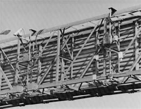
Figure 2. Overhead-mounted detectors above Olson Highway westbound lanes in Minneapolis, MN
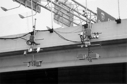
Figure 4. Overhead-mounted detectors above I-4 freeway westbound lanes near Orlando, FL
Figure 5. Overhead detector layout at I-4 freeway site
Figure 6. Overhead detector layout used at I-10 freeway in Phoenix, AZ
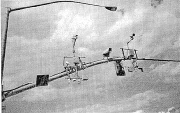
Figure 7. Detectors over southbound lanes at Oracle Road surface street site in Tucson, AZ
Figure 8. Overhead detector array as used at Oracle Road surface street site in Tucson, AZ
Figure 10. Location of inductive loop detectors, self-powered magnetometers,
Traffic Analysis System and CCATS video image processor calibration regions, and ADOT Burle camera field of view on I-10 freeway during Autumn 1993 detector technology evaluations were obtained from the recorded video imagery.
1 ft = 0.305 m
Figure 11. Detection zones on I-10 freeway in Phoenix, AZ during Autumn 1993 detector technology evaluations
2.8 DATA ANALYSIS
The recorded discrete and serial detector data were converted into a comma-delimited format that was compatible with importation into a database program. The data were then read into an easily accessible database using Windows-based Paradox software. In this form, the original recorded data volume was compressed by approximately a factor of two. Selected files were tagged by detector technology, time of run, weather, or data type for further analysis in a program such as Mathcad or with specially written FORTRAN code. Similar parameters from several detectors were plotted as a function of time of day or another independent variable. Selected detector outputs or analysis results, such as detector technology type, traffic parameters (e.g., count, speed, occupancy), and mean and standard deviation of the traffic data parameter, can also be superimposed onto the video imagery recorded during the data collection process to facilitate a qualitative comparison of technology performance.6 The Paradox files will be made available on CD-ROM discs.
2.9 RESULTS
Traffic volume reported by the detectors was compared with volumes established by counting vehicles in the recorded video imagery from several runs. At least two hours of data were manually counted for each test site. The number of runs subjected to this ground truth procedure was increased during subsequent data analysis of all of the runs that will be reported in an addendum to the final report. It was found that the loops at all sites but one gave counts that were usually within 0.5% of the manual counts obtained from the recorded imagery and, thus, the automated loop counts were typically used as reference values against which to compare the counts from other detectors.8 The exception was the Phoenix freeway site where cross talk between loops in the same lane was present. This problem was isolated to the loop wire installation, but no further specific cause for the crosstalk was able to be determined.
There were other instances as well where counts from a detector other than an inductive loop appeared to be closer to the manual count for a particular run or a particular site. In these instances, the automated count from the other detector was used as the standard against which to compare the counts from the rest of the detectors in the run. The manual ground truth value or the automated detector count used as the standard is always referenced in the figure that displays the data. Percent difference is used to denote the variation between data from a given detector and a loop or other detector used as the standard, while percent error denotes the difference between data from a detector and the ground truth value. Run designations are in the form MMDDhhmm, where
MM represents the month, DD the day of the month, hh the hour in which the run began, and mm the minute at which the run began.
2.9.1 Sample of Minneapolis Freeway Results
Run 02110625 is representative of heavy volume morning traffic flow into Minneapolis. The temperature at the start of the run was 18oF (-7.8oC). Light flurries fell during the run.
Figure 12 shows vehicle speed in lane 2 (left eastbound lane of I-394) versus time of day as fitted with a fifth-order polynomial to the actual data. The polynomial fit smoothes out the spiky, discrete nature of the actual speeds. The plotted speeds were calculated by averaging data from the TDN-30, Autoscope 2003, and a pair of inductive loops over 5-minute intervals. The three curves are consistent in their shape, with the only discernible difference being the magnitude of the speed. Speed was measured directly by the Whelen TDN-30 microwave detectors and output via an RS-232 interface to the data logger. The speeds calculated from the loops and the Autoscope VIP used the falling-edge time tag associated with each of two detection zones and knowledge of the spacings between those zones. The speeds noticeably decrease between 6:30 and 7:00 a.m. and resume free flow conditions between 9:30 and 10:00 a.m.
The lower speed calculated from timing of pulses generated by the two-loop speed trap is attributed to a pair of factors. The first is the sequential scanning feature used in the Detector Systems 222B loop driver electronics. The two loops (driven by a single, two-channel card) are alternately turned off and on so as to minimize interference due to crosstalk. This may have caused errors in recording the pulse timing that have a significant impact on the speed calculations. One can envision the lead loop being in the off state when a vehicle passes over it. Then when the loop is energized, the leading edge of the detection pulse does not necessarily correspond to the entrance of the vehicle into the loop’s detection zone.
Figure 12. Comparison of speed data in lane 2 from I-394 Minneapolis freeway site
The second potential error contribution stems from the width of the vehicle detection pulse. According to the loop driver’s specification, the pulse width is 125 ± 25 milliseconds. This pulse width (and the associated 20-percent uncertainty) is a significant fraction of the 170 milliseconds necessary for a vehicle traveling at a freeway speed of 60 mi/h (96.6 km/h) to traverse the 15-foot (4.6-m) center-to-center spacing between the two loops. The maximum percentage error in speed attributed to the pulse-width uncertainty for a vehicle traveling at 60 mi/h (96.6 km/h) is approximately 30 percent. The Traffic Analysis System (TAS) VIP was only operational at the Minnesota I-394 freeway site. Its performance is shown along with that of other detectors in Figures 13 and 14.
Figure 13 displays the vehicle counts from five detectors in lane 2 for a 1-hour ground truth interval during the heavy volume morning traffic flow. The counts from the Autoscope 2003 VIP, TAS VIP, TDN-30 narrow beam microwave Doppler detector, TC-30C ultrasonic detector, and the second 6-foot by 6-foot inductive loop in the lane (controlled by Detector System’s 222B driver) during the 7:00 a.m. to 8:00 a.m. time interval were compared to the ground truth count tabulated manually from video imagery during the post-processing analysis. These detectors were installed to detect vehicles in a zone corresponding to overhead detectors with a 45-degree incidence angle. The counts from the five detectors were within 0.3 to 1.6 percent of the ground truth value in this heavy traffic volume run. The TAS VIP overcounted early in the hour and undercounted for the rest of the
hour, resulting in a 98.8 percent overall count accuracy.
Figure 13. Detector vehicle counts and ground truth in lane 2 at I-394 Minneapolis
freeway site
Figure 14. Detector vehicle counts over 4-hour run duration in lane 2 at I-394 Minneapolis freeway site
Figure 14 shows accumulated vehicle counts in lane 2 for the approximately 4-hour run duration. The counts from the TDN-30 and TC-26 Doppler microwave detectors, TC-30C ultrasonic detector, and TAS video image processor are compared with those from the second inductive loop in the lane. Percent differences were computed using the inductive loop count over the 4- hour interval as the reference.The TDN-30 count is within 0.9 percent of the loop, the TC-30C is within 3.7 percent, and the TAS is within 0.6 percent. The on time of the TC-30C averaged 0.29 second as compared to 0.14 second for the loop. The TC-26 significantly undercounted because of the long electronic hold time characteristic of this detector. The on time of the TC-26 averaged 5.47 seconds. The standard deviation of the TC-26 on time was 6.77 seconds and for the TC-30C it was 0.08 second.
The long hold time of the TC-26 caused missed detections when vehicles were closely spaced, such as in this heavy traffic volume run. The undercount is explained as follows. The TC-26 generates an electronic pulse when a vehicle is detected. If a second vehicle enters the detection zone before the falling edge of the original pulse occurs, then the TC-26 remains in the active state and does not detect the second vehicle as a separate event. Thus, an entire platoon of vehicles may trigger only a single detection pulse. The undercounting is more prevalent during heavy traffic when intervehicle gap times are at their minimum. The almost 5.5-second on time supports the hypothesis that the TC-26 is combining the detection of several vehicles into a single output count. The TAS VIP began the run overcounting vehicles until just after 7 a.m. This may be due to the VIP having difficulty transitioning from dark-to-light ambient lighting conditions. After this time, the TAS showed a tendency to undercount. The net result, a 99.4 percent counting accuracy with respect to the loop, requires explanation. Had the run ended earlier than approximately 10:20 a.m., the percent difference would have been greater because the undercount count interval would not have been long enough to compensate for the initial overcount interval. For example, if the run ended at 8 a.m., the TAS would show a percent difference of approximately +24 percent.
The TAS VIP tended to undercount, except during dark-to-light and light-to-dark transitions when it over-counted. The TAS does allow the operator to adjust a variety of setup and calibration parameters, a feature that theoretically should give more optimal performance in a true operational traffic management scenario. A factor that may have contributed to the observed performance of the TAS was the inability to position an ambient light monitoring zone sufficiently off the roadway due to the camera mounting height and location. Because of the zone’s location, its ambient light monitoring function may have been affected by the headlights from oncoming vehicles.
2.9.2 Sample of Minneapolis Surface Street Results
This March 9 run was notable because of the appreciable amount of snowfall. The run was extended to 6 hours to gather as much data as possible under these conditions. Figure 15 shows vehicle count data output by the detectors in lane 2 (middle through lane on westbound Olson Highway) compared with ground truth obtained by manually counting the vehicles in lane 2 using the recorded video imagery from a 2-hour interval. The results appear within manufacturers' specifications.
2.9.3 Sample of Florida Freeway Results
The data from this July 28 run are representative of morning rush-hour conditions on westbound I-4 into Orlando. The session began at 6:15 a.m. and continued until approximately 10:50 a.m.
Figure 15. Comparison of detector vehicle counts with ground truth in lane 2 of the Olson Highway Minneapolis site
Figure 16. Comparison of detector count data at I-4 Florida freeway site
Figure 16 compares vehicle counts versus time of day for six traffic detectors located in the leftmost lane of the westbound I-4 freeway. Included are detectors that looked straight down (nadir looking) to those that monitored traffic flow 27 feet (8.2 m) further downstream. Vehicle count ground truth was obtained by manually counting vehicles as displayed on the video tape made of the actual run during the 7:30 to 9:00 a.m. interval. The ground truth value was compared with the counts from the detector outputs. The figure includes data from the RTMS-X1 microwave presence radar, a TDN-30 Doppler microwave detector, an SDU-300 ultrasonic detector, an inductive loop, the 780D1000 laser radar, and the Autoscope 2003 video image processor.
A wide variation in the vehicle count is present. The best count results were achieved by the inductive loop, followed by the Schwartz laser radar relay output, the Autoscope VIP, and the Sumitomo SDU-300 ultrasonic detector in that order. The two microwave detectors, the side-looking RTMS and the Whelen TDN-30, showed poor results for this test. The RTMS generally provides better results in the forward-looking orientation. The Whelen TDN-30’s problem was likely due to a failure of a rubber seal that allowed water from a number of thunderstorms to seep into the unit. Whelen has since improved the design of their housings and seals and drilled a hole in the bottom of their case to avoid accumulation of moisture.
2.9.4 Sample of Florida Surface Street Results
Figure 17 shows the short term stability of the vehicle count obtained with the Eltec 833 and the RTMS-X1 in lane 2 (middle westbound lane). The data span almost a 6-hour period starting at 3:53 p.m. on September 7. The weather was hot and humid with heavy rain starting about 5:15 p.m., tapering to thunder showers around 5:30 p.m.
The vehicle counts were accumulated over 3-minute intervals, corresponding to the cycle time of the traffic signals at the intersection of SR436 and an exit ramp from the westbound I-4 freeway. The average value of the count difference was -1.94 counts and the standard deviation of the count difference was 2.83 counts. The standard deviation of the percent difference values was 7.22 percent. The 833 consistently undercounted as evidenced by the predominance of negative percent differences when compared with the RTMS counts. This indicates that the Eltec 833 IR detector was either missing some vehicles entirely (due to insufficient detector sensitivity to distinguish the thermal contrast between the vehicle and the road surface), or failing to discriminate between closely spaced vehicles.
2.9.5 Sample of Phoenix Freeway Results
The data in Figure 18 are from November 22, 1993. The run commenced at 1:59 p.m. when traffic was moderate and continued through the peak traffic period.
The weather was mild and clear. Vehicle count ground truth was obtained by manually counting vehicles on the recorded video imagery for the 4:00 to 5:00 p.m. interval.
The figure shows vehicle flow in lane 2 (middle westbound lane) as calculated using data from the TDN-30 microwave detector, 833 passive infrared, and Autoscope 2003 video image processor. The flows were computed based on one-minute data integration intervals over a one-hour period between 4 and 5 p.m. for which the ground truth vehicle counts were available. The result of using a one-minute integration interval is a discrete, "spiky" curve. Shorter integration intervals, such as thirty seconds, produce flow values that reflect the micro-scopic movement of individual vehicles and thus may generate a curve that shows higher instantaneous flow rates. Short integration intervals may be required when the maximum peak flow on a roadway is needed.
The flow patterns calculated from these detector data generally agree with one another, although the peak values reported by Autoscope at several instances are greater than those from the other detectors. The effect on the accuracy of the vehicle count over the one-hour interval was minimal, however, as the Autoscope count was only one greater than the ground truth value for the interval.
Figure 18. Vehicle Flow in Lane 2 Using Data From TDN-30, 833, and Autoscope
2003 Over 1-Hour Ground Truth Interval at I-10 Phoenix Freeway Site
The EVA VIP was made available for the Summer 1994 detector technology evaluation at Phoenix. Detector counts for the EVA VIP, inductive loop, and RTMS-X1 microwave radar from Run 07281536 are shown in Figures 19 and 20 for lanes 1 and 2, respectively. Lane 1 was the leftmost lane open to all vehicles regardless of passenger occupancy and lane 2 was the middle lane. The temperature was 107oF (41.7oC) at 2 p.m. and 108oF (42.2oC) at 5 p.m. The RTMS microwave radar was used as the basis for count comparison in these graphs because it appeared to be the most accurate vehicle count detector during this run as deduced from the ground truth results. By comparison, the inductive loop in lane 1 overcounted by 6.5 percent, while the loop in lane 2 overcounted by 5.8 percent with respect to the RTMS counts. The EVA, forward-looking RTMS, and the loop were installed to detect vehicles in zones corresponding to overhead detectors with 45-degree (zone 1) or greater (zone 2) incidence angles. The EVA appeared to overcount in lane 1 with respect to the RTMS in daylight and darkness, the overcount being 1.6 percent over the approximately 5-hour run duration. In lane 2, the EVA overcounted until approximately
8:30 p.m. and then undercounted for the rest of the run with respect to the RTMS. In this lane, the total undercount was 3.2 percent. If the run time had been shorter, the overcount in lane 1 attributed to the EVA would be greater, and the undercount in lane 2 would change to an overcount.
Figure 19. Vehicle counts in detector zones 1 and 2 of lane 1 during Run
07281536 at I-10 Phoenix freeway site
Figure 20. Vehicle counts in detector zones 1 and 2 of lane 2 during Run
07281536 at I-10 Phoenix freeway site
2.9.6 Sample of Tucson Surface Street Results
The Tucson evaluation site had the largest assortment of VIPs, three operating in the visible band and one in the infrared. Traffic counts from two of these runs are shown in Figures 21 through 24. Figures 21 and 22 are from lanes 2 (middle) and 3 (curb), respectively, of Run 04121633 on southbound Oracle Road, while Figures 23 and 24 are from Run 04131703 for the corresponding lanes. Lane 3 had a pair of 6-foot (1.8 m) diameter round loops as well as a pair of 6-foot (1.8 m) square loops.
In Figures 21 and 22, vehicle counts from the CCATS-VIP 2 appear lower than those from the other VIPs when darkness occurs. This is due to the particular algorithm in software version E1.01 supplied with the CCATS-VIP 2 that was tested. The E1.01 algorithm was written to prevent shadows from being recognized as vehicles. The algorithm was not able to distinguish all the dark-colored vehicles from the dark background. This phenomenon was observable in the field on the television monitor that showed the traffic flow along with the vehicle counts as overlaid by the VIP. Traficon has since developed software version 2. In their application of the new software to two of the video recordings containing shadows on the road and nighttime operation, Traficon demonstrated an increase in the identification of true vehicles and, thus, increased the true vehicle count between 9 and 20 percent, depending on the conditions of the run.
Data from the Northrop-Grumman imaging infrared traffic sensor overlaps the detection area from the second square inductive loop in lane 3. The Northrop-Grumman sensor undercounted by 22 percent as compared to the loop. However, this particular model of the imaging infrared traffic sensor was not designed to count individual vehicles. It was designed to give a presence output every one second if one or more vehicles was within its detection zone in the preceding 1-second interval. Thus, if two or more vehicles passed through the detection zone during a 1-second interval, only one event would be registered by the sensor. From observation of the traffic flow, it appeared that multiple vehicles did pass through the sensor’s detection zone during some of the 1-second intervals. Additional analysis can be used to verify the more than one vehicle per reporting interval hypothesis by overlaying the vehicle detections onto the video ground truth imagery and examining the correlation of reported and actual events. If the sensor consistently detects the first of two closely spaced vehicles but misses the second, this would indicate that the undercount is indeed due to the particular way the data are processed in the internal algorithms of the sensor. The crisp infrared imagery displayed on the television monitor appears to produce good thermal contrast between the vehicles and the background during day and night operation. This indicates that there is sufficient information in the image to recognize individual vehicles.
The performance of the four video image processors in Run 04131703 is consistent with results from Run 04121633. Figure 23 shows the cumulative vehicle counts for the three visible wavelength VIPs and the second inductive loop in lane 2. These VIPs undercounted, with respect to the loop, by approximately 7 to 10 percent until about 7:00 p.m. as compared with undercounts of 6 to 8 percent the night before. After 7 p.m. the percentage differences between the Autoscope and IDET-100, as compared to the inductive loop, remained fairly constant for the remainder of the run. However, the CCATS-VIP 2 began to miss more vehicle detections after 7:00 p.m. as nighttime darkness occurred. The CCATS reported 18.9 percent fewer counts than did the loop in this run and an undercount of 15.5 percent in the previous night's run. Their updated algorithm should potentially improve upon these results.
Figure 21. Comparison of vehicle counts in lane 2 from VIPs in Run 04121633 at Tucson surface street site
Figure 22. Comparison of vehicle counts in lane 3 from ILDs and VIPs in
Run 04121633 at Tucson surface street site
Figure 23. Comparison of vehicle counts in lane 2 from VIPs in Run 04131703 at Tucson surface street site
Figure 24. Comparison of vehicle counts in lane 3 from ILDs and VIPs in
Run 04131703 at Tucson surface street site
Figure 24 shows lane 3 count results from the same visible spectrum VIPs as were used in monitoring lane 2, as well as from the Northrop-Grumman imaging infrared VIP and the two round inductive loops. The three loops (the second square loop and the two round loops) reported counts within 0.5 percent of each other. The Autoscope count was 5.1 percent below that reported by the second square loop. This result is consistent with the four percent undercount from the previous night's run. Similarly, the IDET-100 overcounted by 6.4 percent as compared to 5.1 percent the night before. Again the counts from the CCATS decreased after 7:00 p.m. The unit reported 23.2 percent fewer counts than the loop as compared to 16.3 percent from Run 04121633. The Northrop-Grumman imaging
infrared sensor undercounted by 19.5 percent compared to 22.1 percent recorded in the previous night’s run. As explained earlier, the Grumman algorithm evaluated in the field tests was not designed to count vehicles, but rather to give a presence output every one second if one or more vehicles was within its detection zone in the preceding 1-second interval.
2.10 CONCLUSIONS
Off-the-shelf, state-of-the-art detectors obtained from various manufacturers
were used to evaluate various detector technologies. Both quantitative and qualitative observations were made regarding how well a particular technology performed relative to others at the field test evaluation sites. Table 6 provides a qualitative summary of which technologies exhibited the best performance with respect to supplying various traffic parameters. These results are based on the limited number of runs reduced so far and the general qualitative opinions gained from using these devices over an 18-month evaluation period. The selection of a detector for traffic management is very much dependent on the specific application. The results obtained in this project may not exactly reflect the performance of newer model detectors, especially those (such as video image processors) that employ software to analyze and report data since software upgrades can significantly
affect detector performance.
Table 6. Qualitative assessment of best performing technologies for gathering specific data
| Technology |
Low-Volume Count |
High-Volume Count |
Low-Volume Speed |
High-Volume Speed |
Best In InclementWeather |
| Ultrasonic |
– |
– |
– |
– |
– |
| Microwave Doppler* |
 |
|
|
|
|
| Microwave True Presence |
|
|
|
|
|
| Passive Infrared |
– |
– |
– |
– |
– |
| Active Infrared |
– |
– |
– |
– |
– |
| Visible VIP |
|
|
|
|
– |
| Infrared VIP |
|
|
|
|
|
| Acoustic Array |
– |
– |
|
|
|
| SPVDMagnetometer |
|
– |
– |
– |
|
| Inductive Loop |
|
|
– |
– |
|
Indicates the best performing
technologies.
– Indicates performance not among the best, but may still be adequate for the
application.
No entry indicates not enough data reduced to make a judgment.
* Does not detect stopped vehicles.
2.10.1 Most Accurate Vehicle Count for Low Traffic Volume
2.10.1 Most Accurate Vehicle Count for High Traffic Volume
Most of the detectors gave good results when used under light traffic conditions. Detectors with multiple outputs or detection zones give the appearance of better performance than do those with only one detection zone because only the most accurate of the outputs was displayed in the reported results. For example, if loop #1 showed better agreement with the ground truth value than loop #2 (for the same lane), then the loop #1 results were presented. Likewise, if a single traffic detector had multiple detection zones, the most favorable of the outputs was used in the plotted results. This affords a greater opportunity for these devices to appear in a favorable light, whereas, a simple detector having a single relay output was represented solely on the basis of that single output.
The ultrasonic and infrared detectors exhibit count accuracies that make them suitable for a variety of applications, but they were typically not among the most accurate. The SPVD magnetometer performed well in low-volume applications, as demonstrated by the zero-percent error over a 2-hour run during snowfall conditions for one of the Minnesota surface-street runs.
Microwave detectors were also well suited to low-volume conditions. The presence-type microwave radar consistently provided better vehicle count results in forward-looking operation than in side-looking orientation. Forward-looking count accuracies to within 1-percent were not uncommon; however, these accuracies were typically provided by only a single detection zone due to the difficulty in confining the detector’s elliptical beam footprint to a single lane of traffic. Because of this footprint geometry, only one detection zone tends to be optimally matched to the dimensions of the traffic lane, while the remainder of the zones tend to undercount (in the narrow parts of the beam where the detection zones are not as wide as the lane) or overcount (where the wide part of the beam tends to spill over into adjacent lanes of traffic).
Doppler-type microwave detectors fare well in low-to-moderate traffic volume conditions, where free-flowing traffic consistently provides a component of motion in the detector's viewing direction that is necessary for the operation of these units. However, there can conceivably be traffic management applications where a knowledge of decreasing speeds can be used to infer that stopped vehicles are present even though the Doppler detector does not give an output indication once the vehicle comes to a full stop. Again, care must be taken to ensure that the detector’s beam footprint on the roadway is confined to the desired monitoring area.
Some video image processors exhibit counting characteristics similar to microwave detectors. The Autoscope 2003, for example, can be configured to have three separate detection zones per lane (two emulating a pair of inductive loops and a third configured as a speed trap). Data show that count results tend to be optimized for a given zone.
Inductive loops are among the most consistent performers, with count accuracies typically in the 99-percent range. Even so, problems with crosstalk and double- or triple-counting large trucks and tractor-trailer rigs have been seen when reviewing videotapes of the field tests.
2.10.2 Most Accurate Vehicle Count for High Traffic Volume
Many of the same observations made in the previous section apply here as well. However, the electronic hold time of a detector begins to become an important factor when intervehicle gap times decrease. The hold time is the period over which a detector remains in the active state after the initial detection of a vehicle.
For the field tests, the hold time of each device was always set to its minimum value. Increasing the hold time in heavy traffic conditions has a negative impact on count accuracy due to the detector's inability to determine when one vehicle departs the detection zone and another enters. With long hold times, a second vehicle enters the detection zone prior to the falling edge of the pulse created by the first vehicle. This can result in several closely spaced vehicles registering only a single count on a given detector. Although several detectors evaluated were designed with long hold times because of an initial traffic management requirement, devices of similar types can certainly be redesigned with shorter hold times as new applications arise.
2.10.3 Most Accurate Speed for Low Traffic Volume
Speed accuracy is a difficult parameter to assess due to the challenge of obtaining the true speeds against which to compare the detector speed outputs. Some detectors compute speeds based on average vehicle lengths. Such devices may yield acceptable accuracies for average vehicle speed over long time intervals, but not for applications that require speeds over short, tactical time intervals or speeds on a vehicle-by-vehicle basis. The latter requirement favors the implementation of detectors that make direct speed measurements, or pairs of detectors that can be used in a speed-trap configuration.
The simplest and most accurate way to measure speed is with a detector that provides it directly, such as a Doppler microwave detector. Doppler devices require a component of vehicle motion in the direction of travel monitored by the detector. Since free-flowing traffic is normally available in low-volume conditions, a Doppler device would seem a logical choice for such an application. Speed as measured by Doppler microwave detectors usually agreed within 2 to 3 mi/h (3.2 to 4.8 km/h) with readings from the speedometers of the probe vehicles. However, the imprecision associated with a human observer recording these values from an analog speedometer of unknown accuracy yields, at best, a reference value and not absolute truth.
Some detectors that provide speed outputs could not be evaluated with the single probe vehicle. These units output average speed data collected over a larger integration interval and, as such, do not give information on a per vehicle basis. Among these devices were several video image processors and the RTMS-X1 microwave true-presence radar.
The selection of a preferred speed-measurement technology is application-dependent. If the requirement is for a unit that will supply average speed, occupancy, or some other statistically derived parameter, the choice should be one of the sophisticated detection systems employing enough processing capability to accurately compute the desired parameter(s). Conversely, if the data are required on a per vehicle basis, the choice narrows to devices that output the desired parameters in real time as they are acquired. Certainly the more sophisticated units, such as video image processors, multi-zone radars, and laser radars, have the ability to output data on a per vehicle basis as they must measure the characteristics of individual vehicles in order to produce their statistical outputs. However, the cost of these units will likely dictate that they be utilized only for applications that require statistical data or where their cost can be justified on an equivalent per detector basis or through life-cycle cost considerations.
2.10.4 Most Accurate Speed for High Traffic Volume
Many of the same points made for low traffic volume apply here as well. The main difference in requirements between low-and high-volume applications stems from the change in vehicle speeds. Vehicles in low-volume conditions are likely to be free-flowing and unconstrained in their movements, while vehicles in high-volume conditions, where the roadway is at or near its designed capacity, will be restricted in their speed. When the traffic demand exceeds the capacity of the roadway, speeds will obviously decrease. If the speeds slow significantly and bumper-to-bumper traffic conditions ensue, then Doppler detectors will not perform when the vehicle speed is below approximately 3 mi/h (4.8 km/h). In some applications, this may not be of concern as the necessity for zero speed measurement may decrease once the traffic flow falls below some fixed threshold.
2.10.5 Best Performance in Inclement Weather
The detectors that seemed the most impervious to inclement weather conditions were the microwave detectors. No appreciable change in performance was noted during conditions such as rain, snow, wind, and extreme cold or heat. The magnetometers performed well in the snow during the Minneapolis surface street tests. The inductive loops, when properly installed, performed reliably through a broad spectrum of weather conditions.
The technologies with the greatest extreme weather limitations include the ultrasonic, infrared, acoustic, and video image processors. This is not due to any flaw in the design of these units, but rather to physical limitations caused by weather-related phenomena, such as gusty winds (greater than 56 mi/h [>25 m/s] in the case of the Doppler ultrasound detector) or the presence of atmospheric obscurants. However, even these devices are relatively unaffected by inclement weather conditions when operating at the short ranges typically associated with their normal traffic management applications.
2.10.6 Microscopic Single-Lane Versus Macroscopic Multiple-Lane Data
Several of the detectors were better suited for collecting data that characterized individual vehicles in multiple lanes, while others were better for gathering data from groups of vehicles in multiple lanes. The detectors best suited for acquiring microscopic (individual vehicle) data over multiple lanes were the true-presence microwave radar and the video image processors. Those useful for collecting macroscopic (groups of vehicles) data were the wide-beam Doppler microwave detectors, true-presence microwave radar, and the video image processors. The selection of a particular detector is highly dependent on the specific application.
Previous | Next
| 

