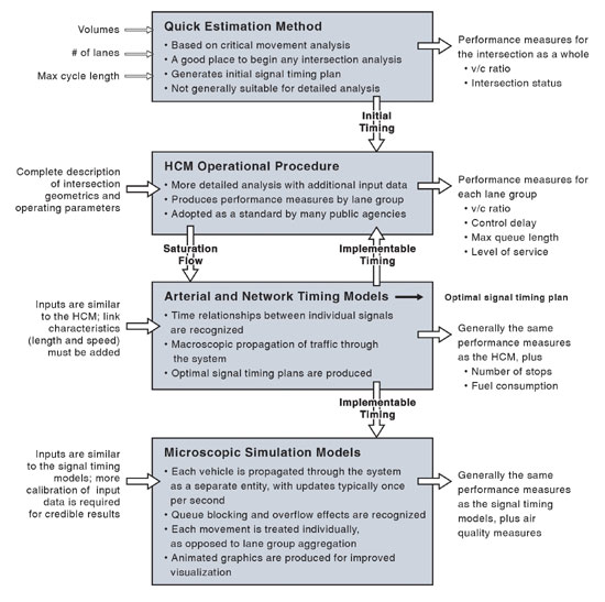
7.0 Operational Analysis Methods

Chapter 6 described tools that can be used to assess the safety performance at a signalized intersection. Evaluating a candidate treatment usually requires that its performance also be assessed from the perspective of traffic operations. This chapter will, therefore, focus on measures for assessing operational performance and computational procedures used to determine specific values for those measures.

The relationships between safety performance and operational performance are difficult to define in general terms. Some intersection treatments that would improve safety might also improve operational performance, but others might diminish operational performance. Furthermore, the nature of safety and operational measures makes them difficult to combine in a way that would represent both perspectives.

Operational performance measures tend to be fewer in number and more easily related to site-specific conditions than are safety performance measures. The computations themselves are more amenable to deterministic models, and a wide variety of such models, mostly software based, is available. Selecting a model for a specific purpose is generally based on the tradeoff between the difficulty of applying the model and the required degree of accuracy and confidence in the results. The degree of application difficulty is reflected in the required amount of site-specific data as well as the level of personnel time and training needed to apply the model and to interpret the results.

Recent user interface enhancements in the more advanced traffic model software products have made the products much easier to apply; some can generate animated graphics displays depicting the movement of individual vehicles and pedestrians in an intersection (an example is in figure 53). An increasing trend toward the use and acceptance of advanced traffic modeling techniques has occurred as a result of these enhancements.

While the range of operational performance models is more or less continuous, it will be categorized into the following four analysis levels for purposes of this discussion:

These levels are listed in order of complexity and application difficulty, from least to greatest. They are summarized in figure 54 in terms of their inputs, outputs and the data that may flow between them. Each analysis levels will be discussed separately.

The process for evaluating the operational performance of an intersection remains unchanged regardless of the analysis level and the issues at hand. The analysis should begin at the highest level and should continue to the next level of detail until the key operations-related issues and concerns have been addressed in sufficient detail.

Figure 53. Still reproduction of a graphic from an animated traffic operations model.

The ability to measure, evaluate, and forecast traffic operations is a fundamental element of effectively diagnosing problems and selecting appropriate treatments for signalized intersections. A traffic operations analysis should describe how well an intersection accommodates demand for all user groups. Traffic operations analysis can be used at a high level to size a facility and at a refined level to develop signal timing plans. This section describes key elements of signalized intersection operations and provides guidance for evaluating results.

7.1 Operational measures of Effectiveness

Three measures of effectiveness are commonly used to evaluate signalized intersection operations:

The HCM 2000 estimates measures of effectiveness by lane group.⁽²⁾ A lane group includes a movement or movements that share a common stop bar. Exclusive turn lanes are generally treated as individual lane groups (i.e., right-turn-only lane). Shared movements (such as one or more through lanes that are also serving right turns) are represented as a single lane group. Lane group results can be aggregated by approach and for an entire intersection.

Other international capacity analysis procedures, including the Australian-based SIDRA software analysis package,⁽⁷⁰⁾ the Canadian capacity guide,⁽⁷¹⁾ and the swedish capacity guide,⁽⁷²⁾ provide methods for estimating performance measures at the individual lane level. These procedures implicitly assume an equal volume-to-capacity (v/c) ratio across “choice lanes” (i.e., a through and a through/right-turn lane).

Figure 54. Overview of intersection traffic analysis models.

7.1.1 Motor vehicle Capacity and Volume-to-Capacity Ratio

Capacity is defined as the maximum rate at which vehicles can pass through a given point in an hour under prevailing conditions; it is often estimated based on assumed values for saturation flow. Capacity accounts for roadway conditions such as the number and width of lanes, grades, and lane use allocations, as well as signalization conditions. Under the HCM 2000 procedure, intersection capacity is measured for critical lane groups (those lane groups that requires the most amount of green time). Intersection volume-to-capacity ratios are based on critical lane groups; noncritical lane groups do not constrain the operations of a traffic signal. Rules for determining critical lane groups are further explained in HCM 2000.

Research conducted as part of the 1985 HCM showed that the capacity for the critical lanes at a signalized intersection was approximately 1,400 vehicles per hour.⁽⁷³⁾ This capacity is a planning-level estimate that incorporates the effects of loss time and typical saturation flow rates. Studies conducted in the state of Maryland have shown that signalized intersections in urbanized areas have critical lane volumes upwards of 1,800 vehicles per hour.⁽⁷⁴⁾

The v/c ratio, also referred to as degree of saturation, represents the sufficiency of an intersection to accommodate the vehicular demand. A v/c ratio less than 0.85 generally indicates that adequate capacity is available and vehicles are not expected to experience significant queues and delays. As the v/c ratio approaches 1.0, traffic flow may become unstable, and delay and queuing conditions may occur. Once the demand exceeds the capacity (a v/c ratio greater than 1.0), traffic flow is unstable and excessive delay and queuing is expected. Under these conditions, vehicles may require more than one signal cycle to pass through the intersection (known as a cycle failure). For design purposes, a v/c ratio between 0.85 and 0.95 generally is used for the peak hour of the horizon year (generally 20 years out). Overdesigning for an intersection should be avoided due to negative impacts to pedestrians associated with wider street crossings, the potential for speeding, land use impacts, and cost.

7.1.2 Motor vehicle Delay and Level of Service

Delay is defined in HCM 2000 as “the additional travel time experienced by a driver, passenger, or pedestrian.”⁽²⁾ The signalized intersection chapter (chapter 16) of the HCM provides equations for calculating control delay, the delay a motorist experiences that is attributable to the presence of the traffic signal and conflicting traffic. This includes time spent decelerating, in queue, and accelerating.

The control delay equation comprises three elements: uniform delay, incremental delay, and initial queue delay. The primary factors that affect control delay are lane group volume, lane group capacity, cycle length, and effective green time. Factors are provided that account for various conditions and elements, including signal controller type, upstream metering, and delay and queue effects from oversaturated conditions.

Control delay is used as the basis for determining LOS. Intersection control delay is generally computed as a weighted average of the average control delay for all lane groups based on the amount of volume within each lane group. Caution should be exercised when evaluating an intersection based on a single value of control delay because this is likely to over- or underrepresent operations for individual lane groups. Delay thresholds for the various LOs are given in table 33.

Table 33. Motor vehicle LOs thresholds at signalized intersections⁽²⁾

7.1.3 Motor vehicle Queue

Vehicle queuing is an important measure of effectiveness that should be evaluated as part of all analyses of signalized intersections. Estimates of vehicle queues are needed to determine the amount of storage required for turn lanes and to determine whether spillover occurs at upstream facilities (driveways, unsignalized intersections, signalized intersections, etc.). Approaches that experience extensive queues also are likely to experience an overrepresentation of rear-end collisions.

Vehicle queues for design purposes are typically estimated based on the 95^th percentile queue that is expected during the design period. Appendix G to chapter 16 of the HCM 2000 provides procedures for calculating back of queue. In addition, all known simulation models provide ways of obtaining queue estimates.

7.1.4 Transit Level of Service

The assessment of transit capacity and quality of service is the subject of its own reference document, the Transit Capacity and Quality of Service Manual.⁽⁷⁵⁾ In addition, on-street elements from that document are presented in the HCM 2000 in chapters 14 and 27.⁽²⁾ Space does not permit the reproduction of these elements in this document; therefore the reader is encouraged to review these references for more information on the variety of quality-of-service measures and capacity estimation techniques available.

7.1.5 Bicycle Level of Service

The HCM 2000 provides an analysis procedure for assessing the LOS for bicycles at signalized intersections where there is a designated on-street bicycle lane on at least one approach. This section replicates the procedure from chapter 19 of the HCM 2000.

Many countries have reported a wide range of capacities and saturation flow rates for bicycle lanes at signalized intersections. The HCM 2000 recommends the use of a saturation flow rate of 2,000 bicycles per hour as an average value achievable at most intersections. This rate assumes that right-turning motor vehicles yield the right-of-way to through bicyclists. Where aggressive right-turning traffic exists, this rate may not be achievable, and local observations are recommended to determine an appropriate saturation flow rate.

Using the default saturation flow rate of 2,000 bicycles per hour, the capacity of the bicycle lane at a signalized intersection may be computed using equation 6:

(6)

At most signalized intersections, the only delay to bicycles is caused by the signal itself because bicycles have right-of-way over turning motor vehicles. Where bicycles are forced to weave with motor vehicle traffic or where bicycle right-of-way is disrupted due to turning traffic, additional delay may be incurred. Control delay is estimated using the first term of the delay equation for motor vehicles at signalized intersections, which assumes that there is no overflow delay. This is reasonable in most cases, as bicyclists will not normally tolerate an overflow situation and will use other routes. This control delay is estimated using equation 7:

(7)

Table 34 indicates LOS criteria for bicycles at signalized intersections on the basis of control delay.

Table 34. Bicycle LOs thresholds at signalized intersections.⁽²⁾

7.1.6 Pedestrian Level of Service

In the HCM 2000 (chapter 18), pedestrian LOs is determined based on the average delay per pedestrian (i.e., wait time). Pedestrian delay is calculated using two parameters: cycle length and effective green time for pedestrians. In the absence of field data, the HCM 2000 recommends estimating effective green time for pedestrians by taking the walk interval and adding 4 seconds of the flashing DON’T WALK interval to account for pedestrians who depart the curb after the start of flashing DON'T WALK. Equation 8 shows the equation for calculating pedestrian delay based on equation 18-5 of the HCM 2000:

(8)

Table 35 indicates the LOs thresholds for pedestrian crossings at signalized intersections.

Table 35. Pedestrian LOs thresholds at signalized intersections.⁽²⁾

Figure 55 illustrates the amount of effective green time required for pedestrians to achieve each LOs threshold based on a specified cycle length. As shown in the figure, the amount of green time required for pedestrian crossings to meet a LOS D standard increases with longer cycle lengths. For cycle lengths in excess of 150 seconds, a minimum pedestrian effective green time of 40 seconds is required to maintain LOS D.

Note: FDW = Flashing “DON’T WALK”

Figure 55. Pedestrian LOs based on cycle length and minimum effective pedestrian green time.(2)

7.2     Traffic Operations Elements

Signalized intersection operations are a function of three elements described in the following sections along with a discussion on their effect on operations.

7.2.1    Traffic Volume Characteristics

The traffic characteristics used in an analysis can play a critical role in determining intersection treatments. Overconservative judgment may result in economic inefficiencies due to the construction of unnecessary treatments, while the failure to account for certain conditions (such as a peak recreational season) may result in facilities that are inadequate and experience failing conditions during certain periods of the year.

An important element of developing an appropriate traffic profile is distinguishing between traffic demand and traffic volume. For an intersection, traffic demand represents the arrival pattern of vehicles, while traffic volume is generally measured based on vehicles’ departure rate. For the case of overcapacity or constrained situations, the traffic volume may not reflect the true demand on an intersection. In these cases, the user should develop a demand profile. This can be achieved by measuring vehicle arrivals upstream of the overcapacity or constrained approach. The difference between arrivals and departures represents the vehicle demand that does not get served by the traffic signal. This volume should be accounted for in the traffic operations analysis.

Traffic volume at an intersection may also be less than the traffic demand due to an overcapacity condition at an upstream or downstream signal. When this occurs, the upstream or downstream facilities “starve” demand at the subject intersection. This effect is often best accounted for using a microsimulation analysis tool.

7.2.2 Intersection Geometry

The geometric features of an intersection influence the service volume or amount of traffic an intersection can process. A key measure used to establish the supply of an intersection is saturation flow, which is similar to capacity in that it represents the number of vehicles that traverse a point per hour; however, saturation flow is reported assuming the traffic signal is green the entire hour. By knowing the saturation flow and signal timing for an intersection, one can calculate the capacity (capacity = saturation flow times the ratio of green time to cycle length). Saturation headway is determined by measuring the average time headway between vehicles that discharge from a standing queue at the start of green, beginning with the fourth vehicle.⁽²⁾ Saturation headway is expressed in time (seconds) per vehicle.

Saturation flow rate is simply determined by dividing the average saturation headway into the number of seconds in an hour, 3,600, to yield units of vehicles per hour. The HCM 2000 uses a default ideal saturation flow rate of 1,900 vehicles per hour. Ideal saturation flow assumes 3.6-m (12-ft)-wide travel lanes, through movements only, and no curbside impedances, pedestrians/bicyclists, grades, or central business district influences. The HCM 2000 provides adjustment factors for nonideal conditions to estimate the prevailing saturation flow rate. Saturation flow rate can vary in time and location. Saturation flow rates have been observed to range between 1,500 and 2,000 passenger cars per hour per lane.⁽²⁾ Given the variation that exists in saturation flow rates, local data should be collected where possible to increase the accuracy of the analysis.

Existing or planned intersection geometry should be evaluated to determine features that may impact operations and that require special consideration.

7.2.3 Signal Timing

The signal timing of an intersection also plays an important role in its operational performance. Key factors include:

7.3 Rules of Thumb for Sizing an intersection

This is the first level of analysis. It is the only level that does not use formal models or procedures. Instead, it relies on the collective experience of past practice. As such, it offers only a very coarse approximation of a final answer.

In spite of its obvious limitations, this approach can be used to size an intersection and determine appropriate lane configurations. The literature provides guidelines, shown in table 36, for determining intersection geometry at the planning level.

Table 36. Planning-level guidelines for sizing an intersection.

7.4 Critical movement analysis

Critical movement analysis (CMA) is usually applied at the planning stage; represents the highest of the 4 levels of operational performance models. Various versions of CMA procedures have been widely used over the past 20 years, including:

The QEM procedures can be carried out by hand, although software implementation is much more productive. The computations themselves are somewhat complex, but the minimal requirement for site-specific field data (traffic volumes and number of lanes) is what puts the QEM into the category of a simple procedure. While the level of output detail is simplified in comparison to more data-intensive analysis procedures, the QEM provides a useful description of the operational performance by answering the following questions:

Figure 56. Graphical summary of the Quick Estimation Method.

Step 1 -Identify movements to be served and assign hourly traffic volumes per lane. This is the only site-specific data that must be provided. The hourly traffic volumes are usually adjusted to represent the peak 15-minute period. The number of lanes must be known to compute the hourly volumes per lane.

Step 2 -Arrange the movements into the desired signal phasing plan. The phasing plan is based on the treatment of each left turn (protected, permitted, etc.). The actual left-turn treatment may be used, if known. Otherwise, the likelihood of needing left-turn protection on each approach will be established from the left-turn volume and the opposing through traffic volume.

Step 3 -Determine the critical volume per lane that must be accommodated on each phase. Each phase typically accommodates two nonconflicting movements. This step determines which movements are critical. The critical movement volume determines the amount of time that must be assigned to the phase on each signal cycle.

Step 4 -Sum the critical phase volumes to determine the overall critical volume that must be accommodated by the intersection. This is a simple mathematical step that produces an estimate of how much traffic the intersection needs to accommodate.

Step 5 -Determine the maximum critical volume that the intersection can accommodate: This represents the overall intersection capacity. The HCM QEM suggests 1,710 vph for most purposes.

Step 6 -Determine the critical volume-to-capacity ratio, which is computed by dividing the overall critical volume by the overall intersection capacity, after adjusting the intersection capacity to account for time lost due to starting and stopping traffic on each cycle. The lost time will be a function of the cycle length and the number of protected left turns.

Step 7 -Determine the intersection status from the critical volume-to-capacity ratio. The status thresholds are given in table 37.

Table 37. V/C ratio threshold descriptions for the Quick Estimation Method.⁽²⁾

Understanding the critical movements and critical volumes of a signalized intersection is a fundamental element of any capacity analysis. A CMA should be performed for all intersections considered for capacity improvement. The usefulness and effectiveness of this step should not be overlooked, even for cases where more detailed levels of analysis are required. The CMA procedure gives a quick assessment of the overall sufficiency of an intersection. For this reason, it is useful as a screening tool for quickly evaluating the feasibility of a capacity improvement and discarding those that are clearly not viable.

Some limitations of Comma procedures in general, and the QEM in particular:

7.5 HCM Operational Procedure for Signalized Intersections

For many applications, performance measures such as vehicle delay, LOS, and queues are desired. These measures are not reported by the Comma procedures, but are provided by macroscopic-level procedures such as the HCM operational analysis methodology for signalized intersections. This procedure is represented as the second analysis level in figure 54. Macroscopic-level analyses provide results over multiple cycle lengths based on hourly vehicle demand and service rates. HCM analyses are commonly performed for 15-minute periods to accommodate the heaviest part of the peak hour.

The HCM analysis procedures provide estimates of saturation flow, capacity, delay, LOS, and back of queue by lane group for each approach. Exclusive turn lanes are considered as separate lane groups. Lanes with movements that are shared are considered a single lane group. Lane group results can be aggregated to estimate average control delay per vehicle at the intersection level.

The increased output detail compared to the Comma procedure is obtained at the expense of additional input data requirements. A complete description of intersection geometrics and operating parameters must be provided. Several factors that influence the saturation flow rates (e.g., lane width, grade, parking, pedestrians) must be specified. A complete signal operating plan, including phasing, cycle length, and green times, must be developed externally. As indicated in figure 54, an initial signal operating plan may be obtained from the QEM, or a more detailed and implementable plan may be established using a signal timing model that represents the next level of analysis. Existing signal timing may also be obtained from the field.

In addition to the signalized intersection procedure, the HCM also includes procedures to estimate the LOS for bicyclists, pedestrians, and transit users at signalized intersections. These have been discussed previously in this chapter.

Known limitations of the HCM analysis procedures for signalized intersections exist under the following conditions:

• Available software products that perform HCM analyses generally do not accommodate intersections with more than four approaches.

• The analysis may not be appropriate for alternative intersection designs.

• The effect of queues that exceed the available storage bay length is not treated in sufficient detail, nor is the backup of queues that block a stop line during a portion of the green time.

• Driveways located within the influence area of signalized intersections are not recognized.

• The effect of arterial progression in coordinated systems is recognized, but only in terms of a coarse approximation.

• Heterogeneous effects on individual lanes within multilane lane groups (e.g., downstream taper, freeway on-ramp, driveways) are not recognized.

If any of these conditions exist, it may be necessary to proceed to the next level of analysis.

7.6 Arterial and Network Signal Timing Models

As with the HCM procedures, arterial and network signal timing models are also macroscopic in nature. They do, however, deal with a higher level of detail, and are more oriented to operational design than is the HCM. The effect of traffic progression between intersections is treated explicitly, either as a simple time-space diagram or a more complex platoon propagation phenomenon. In addition, these models can explicitly account for pedestrian actuations at intersections and their effect on green time for affected phases.

These models attempt to optimize some aspect of the system performance as a part of the design process. The two most common optimization criteria are quality of progression as perceived by the driver, and overall system performance, using measures such as stops, delay, and fuel consumption. As indicated in figure 54, the optimized signal timing plan may be passed back to the HCM analysis or forward to the next level of analysis, which involves microscopic simulation.

While the signal timing models are more detailed than the HCM procedures in most respects, they are less detailed when it comes to determining the saturation flow rates. The HCM provides the computational structure for determining saturation flow rates as a function of geometric and operational parameters. On the other hand, saturation flow rates are generally treated as input data by signal timing models. The transfer of saturation flow rate data between the HCM and the signal timing models is therefore indicated on figure 54 as a part of the data flow between the various analysis levels.

The additional detail present in the signal timing models overcomes many of the limitations of the HCM for purposes of operational analysis of signalized intersections. It will not generally be necessary to proceed to the final analysis level, which involves microscopic simulation, unless complex interactions take place between movements or additional outputs, such as animated graphics, are considered desirable.

7.7 Microscopic Simulation Models

For cases where individual cycle operations and/or individual vehicle operations are desired, a microscopic-level analysis should be considered to supplement the aggregate results provided by the less detailed analysis levels. Microscopic analyses are performed using one or more of several simulation software products. Microsimulation analysis tools are based on a set of rules used to propagate the position of vehicles from one second to the next. Rules such as car following, yielding, response to signals, etc., are an intrinsic part of each simulation software package. The rules are generally stochastic in nature, in other words there is a random variability associated with each aspect of the operation. Some simulation tools produce animated graphical outputs to illustrate the operating conditions on a vehicle-by-vehicle and second-by-second basis for a given time period. Some simulation models can explicitly model pedestrians, enabling the analyst to study the impedance effects of vehicles on pedestrians and vice versa. However, the pedestrian modeling ability of most simulation programs is quite simplistic and does not capture the full range of pedestrian activity and ability.

Microscopic models produce nominally the same measures of effectiveness as their macroscopic counterparts, although minor differences exist in the definition of some measures. Pollutant discharge measures are typically included in microscopic results. Interestingly, one of the most important measures, capacity, is notably absent from simulation results because the nature of simulation models does not lend itself to capacity computations

Microscopic simulation tools can be particularly effective for cases where intersections are located within the influence area of adjacent signalized intersections and are affected by upstream and/or downstream operations. In addition, graphical simulation output may be desired to verify field observations and/or provide a visual description of traffic operations for an audience. Microscopic simulation tools also can be used to identify the length of time that a condition occurs, and can account for the capacity and delay effects associated with known system-wide travel patterns.

The level of effort involved with developing a microscopic simulation network is considerably greater than that of a macroscopic analysis, and enormously greater than a critical movement analysis. Like the HCM operational procedure, microscopic simulation tools require a fully specified signal-timing plan that must be generated externally. Unlike the HCM, however, an extensive calibration effort using field data is essential to the production of credible results. For this reason, the decision of whether to use a microscopic simulation tool should be made on a case-by-case basis, considering the resources available for acquisition of the software and for collecting the necessary data for calibrating the model to the intersection being studied.

Part III