• Federal Highway Administration >
• Publications >
• Research Publications >
• 04096 >
• 17.Cfm >
• Evaluation of LS-DYNA Wood Material Model 143

Evaluation of LS-DYNA Wood Material Model 143

PDF files can be viewed with the Acrobat® Reader®

17- Developer's Comments on User's Evaluation

This section was written by the developer and begins with topics selected by the developer and previously discussed by the user in chapters 9 through 16. These are topics that the developer concluded were worthy of additional discussion and explanation. These topics and the corresponding developer's comments are briefly tabulated in table 7. Following this table is a more indepth discussion of these topics. For ease of discussion, each topic can be grouped roughly into one of three categories:

1. LS-DYNA code behavior.
2. User's (analyst's) responsibility.
3. Wood model theory or wood model input parameter selection.

Material models, like the wood and soil models, are not stand-alone codes. They are subroutines that work only in conjunction with the LS-DYNA code. Therefore, the results of any analyses performed depend on the formulation of the LS-DYNA code, the user's specification of the geometric mesh and boundary conditions, the user's specification of the input parameter values for various LS-DYNA features and material models, and the formulation and input parameter values for the wood material model.

The user's evaluation chapters demonstrate the behavior of the finite element systems under various operating conditions. By system, we mean the wood material model used in conjunction with other material models/structures and LS-DYNA controls. An example is a vehicle impacting a wood post embedded in a neoprene and concrete support structure. Code issues are related to the functioning of the LS-DYNA features via the LS DYNA controls, which affect the behavior of the system. These controls are independent of the wood model and are typically proprietary in formulation. The user's issues are related to the proper user's setup of the finite element mesh, the user's regard for LS-DYNA diagnostics, and the user's selection of LS-DYNA input parameters. It is the user's responsibility to learn the LS-DYNA code, set up the mesh properly, and input the correct control parameters.

Most calculations documented by the user show good system behavior, with the wood material model behaving realistically. However, some calculations show poor system behavior, which the user did not adequately explain. The user is a potential end user of the code (not a material model or code developer) and, therefore, did not distinguish between LS-DYNA code issues, user's setup and input parameter selection issues, and wood model issues.

Of the 10 topics chosen for discussion, we can categorize 5 as code- and user-related issues, and 5 as wood model issues. No changes to the wood model theory or wood model input parameter values affect the results regarding the five code- and user-related issues. The five wood model issues are:

• Volume expansion and contraction.
• Static post simulation behavior.
• Mesh-size dependency.
• Post breakage and fracture.
• Erosion criteria.

The developer performed many additional calculations that were related to some of these wood model issues, as discussed in section 17.3. The additional calculations indicate that none of the wood model issues are wood model deficiencies that warrant changes to the theoretical formulation of the model. However, changes to the wood model input parameter values may positively affect the results.

The developer wishes to thank the user for providing a detailed report on the initial use of the wood material model. The questions and comments provided by a novice user of the wood model are a good learning tool for other novice users. However, the tone and conclusions (or lack thereof) in some portions of the user's evaluation report in chapters 9 through 16 may leave the reader wondering whether the wood model is ready for use. Both the developer's and the user's wood model evaluation sections were reviewed by individuals at FHWA, NHTSA NCAC, and each COE before publication. One experienced analyst and reviewer stated that he understood that many of the issues brought up by the user were LS-DYNA code and user input parameter selection issues, and not wood model issues. However, a beginning analyst might not make this distinction and think that the model was deficient. This is because the user's evaluation report brings up various issues without thoroughly defining them or resolving them and, more importantly, without identifying how the issue relates to the wood material model.

Therefore, all analytical results provided by the user have been included in this report, whether or not the simulation was performed correctly, and whether or not the problem and solution are directly related to the wood model. As the developer, we believe that this consolidated, comprehensive report provides a very valuable learning tool for analysts who want to learn how to use the wood (or soil) model as part of the LS DYNA code. We think that identifying and providing commentary on issues is a much better approach than removing issues that are not directly related to the wood model. Some of the issues in the user's evaluation report are potential hurdles that other users may run into and, therefore, warrant publication. We hope that the following discussion provides inexperienced users with guidelines on how to correctly run the wood model.

It is the developer's opinion that the user's wood model evaluation revealed no substantial problems with the model. In fact, the developer performed various analyses to positively determine that none of the issues were model deficiencies. The developer has demonstrated that all of the user's evaluation calculations gave reasonable results when reasonable LS-DYNA control parameters and reasonable wood input parameters were used. In particular, see section 17.3 for a thorough discussion of the excessive erosion problem and solution, and a discussion of post breakage.

17.1 - Table of Wood Model Topics

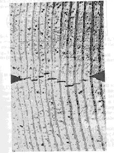
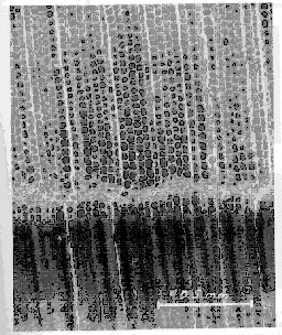
17.2 - Discussion of Wood Model Topics

These items are listed in the order that they were brought up by the user in chapters 9 through 16.

Volume Expansion and Contraction: The user demonstrates that the volume of the single elements pulled in tension expands by as much as 6 percent (previously shown in figure 73). The user believes that there should be no change in volume for wood (i.e., wood is incompressible, but shows no credible data or peer-reviewed documentation to support this position). It is the developer's position that Poisson's ratios measured by FPL and reported in the literature(¹¹) do not support the assumption of incompressibility. Therefore, modeling wood as an incompressible material is not recommended by the developer.

The suite of clear wood data provided by FPL (documented in the user's manual)(²) included measurement of the major Poisson's ratio in the elastic region. A transversely isotropic material such as wood has three ratios. Typical values are around ν_LT = 0.16, ν_TL = 0.004, and ν_TR = 0.4 for pine at the fiber saturation point. No measurements were reported for the effective Poisson's ratios in the plastic/damage regions (once the material yields or softens). By effective Poisson's ratio, we mean the ratio of the lateral strain to the axial strain in uniaxial stress tests (without lateral confinement). Porous materials tend to flow during yielding and softening, which can result in an effective Poisson's ratio that is larger or smaller than the elastically measured value. For example, for porous geological materials such as concrete, the effective Poisson's ratio is typically modeled as greater than the elastic ratio in unconfined compression (with values greater than 1) and less than the elastic ratio in unconfined tension. The effective ratio depends on the shape of the yield surfaces, coupling of the yield surfaces, and how the plasticity algorithm is formulated.

To achieve no change in volume, the elastic and effective Poisson's ratios would have to be 0.5. The FPL data indicate that the elastic Poisson's ratios are not 0.5. However, no lateral strain or change in the volume measurements is available to confirm or refute an effective Poisson's ratio of 0.5 in the plastic region. Therefore, we recommend that any future test data generated (such as uniaxial tension and compression tests) include lateral strain measurements.

For a material to be modeled as incompressible in the elastic region, it must also be modeled as isotropic. By examining the elastic constitutive equations in the wood model user's manual,(²) one can readily determine that all Poisson's ratios can only be equal to 0.5 when all stiffnesses (parallel and perpendicular) are equal. Wood, on the other hand, is modeled as transversely isotropic (a simplification of orthotropic) because the stiffness parallel to the grain is about 50 times greater than that perpendicular to the grain.

Another point to note is that the volume change being modeled implicitly includes expansion and compaction of pores and the opening up of fracture surfaces. This is demonstrated schematically in figure 101. The formation of voids and the compaction of pores are shown in figure 102. The fracture of wood creates voids, which are modeled as volume expansion with continuum models like the wood model. Wood is also porous. The crushing of pores is modeled as volume compaction.

(a) Fracture of wood (specimen breaks in two)

(b) Finite element simulation (element stretches)

Figure 101. Schematic demonstration of how a finite element treats fracture prior to erosion.

(a) Void formation(11)

(b) Pore compaction(11)

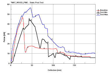
Figure 102. Demonstration of void formation and crushing of wood specimens.

Setting the compressibility or effective Poisson's ratio behavior of the wood model is not simply a matter of specifying an input value. Rather, it requires changes to the formulation of the model to include coupling between the parallel (axial) plasticity and perpendicular (lateral) plasticity. The current wood model includes separate yield surfaces and plasticity computations for yielding parallel and perpendicular to the grain. As a result, yielding parallel to the grain does not induce plastic flow perpendicular to the grain. Similarly, yielding perpendicular to the grain does not include plastic flow parallel to the grain. We recommend exploring and implementing methods of coupling the plastic flow once sufficient test data are generated to set the coupling via measurement of the effective Poisson's ratio or volume change.

Static Post Simulations: The user states that, during fracture, the wood model is too weak: Once the post begins to fail, the simulation forces fall below the minimum force levels seen in testing. As the developer, we disagree. Comparison of the simulation force histories with data (as opposed to performance envelopes) demonstrates that the simulation forces are not too low. In addition, excellent correlations between the simulations and the performance envelopes are achieved through careful selection of the input fracture energy. No changes to the material model formulation are required to achieve good agreement between the simulations and the static post test data. We suggest that the user plot all data curves in comparison to the performance envelopes and more thoroughly discuss their performance envelope selection process. The static data are highly scattered and display both brittle and ductile behaviors.

Figure 103. User's grades 1 and 1D simulation compared to the performance envelopes, using G_{f II} = 50 G_f .

(a) Set 1

(b) Set 2

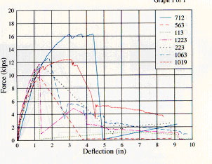
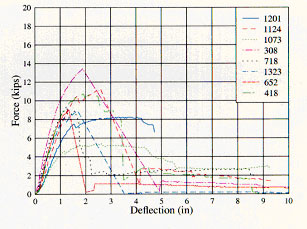
Figure 104. Most of the grades 1 and 1D static post test measurements exhibit brittle behavior.

The user's simulation and performance envelopes are shown in figure 103. The suite of test data used to generate these performance envelopes is shown in figure 104 for grades 1 and 1D. The simulation conducted by the user peaks at about 47 MPa, then softens in a brittle mode between 25 and 50 mm of deflection. The behavior of the simulation is similar to 9 out of 15 of the data curves shown in figure 104, which fail in a brittle mode between 25 and 50 mm of deflection. This is good agreement.

However, it is evident that the user's simulation fails in a more brittle manner than that represented by the performance envelopes. The user supposedly constructed the envelopes using curves from posts that exhibited the most typical behavior. The minimum and maximum curves, which define the performance envelopes, do not represent any one particular curve from the tests. The simulation was conducted using the default fracture energies recommended by the developer.

Good agreement between the simulation and the performance envelopes can be achieved by increasing the parallel-to-the-grain fracture energy above the default value (as shown in figure 105). Refer to chapter 5 for a thorough review of the developer's static post simulations. Simulations conducted at two different fracture energies were previously shown in figure 22. The calculation with G_{f II} = 50 G_f (green dotted line) agrees with the brittle data. The calculation with G_{f II} = 250 G_f (red solid line) agrees with the ductile data. It is important to note that the default fracture energy for saturated room-temperature pine is based on correlations with the dynamic (bogie impact) performance envelopes. A higher value than the default is needed to achieve good correlations with the static performance envelopes.

Figure 105. Good correlation is achieved between the simulation and the performance envelopes
by increasing the fracture energy above the default value (to G_{f II} = 250 G_f ).

Mesh-Size Dependency: The user suggests that the wood model is mesh-size dependent because static post calculations conducted at two different mesh refinements (25.4-mm and 12.7-mm elements) exhibit different late-time force-deflection behaviors. These behaviors were previously shown in figure 78.

It is not clear to the developer that the origin of the different late-time responses is the wood model, rather than the overall (geometric/material/contact) model. The user demonstrated mesh-size sensitivity of a finite element system. However, the user did not demonstrate that the sensitivity was a result of the wood model formulation. The origin of the different responses is an issue because the developer could possibly adjust the model formulation if the material model is the source of the different responses, otherwise, the geometric model must be adjusted.

Often, material models exhibit mesh-size sensitivity because of their softening formulations. However, the developer included coding to regulate mesh-size sensitivity by making the softening formulation of the wood model a function of element size and checking this behavior for single elements. The softening formulation of the wood model for single elements does not depend on element size. In addition, the user's early-time force-deflection behaviors are in good agreement for peak strength and initial softening, which suggests that the softening formulation has been adequately regulated.

On the other hand, the developer's static post calculations discussed in chapter 5 (for example, see figure 27) indicate that the late-time behavior is the most sensitive portion of the simulations. For example, the late-time behavior is sensitive to input parameter selection, hourglass control, element formulation, and geometric modeling details. In fact, two other reviewers suggested that the perceived mesh-size sensitivity is not an issue because the discrepancy in the response occurs at a late time, where data are not adequately measured.

We note that the deformed configurations in the user's plots look different in the region where the post is rolling over the rounded edge on the brace. It appears that more wood compaction is taking place at this location in the crude mesh than in the refined mesh. Therefore, the source of the sensitivity could also be a result of modeling details in this region.

We recommend reexamining this calculation in the future to determine the source of the mesh-size sensitivity. If the wood model is the source of the sensitivity, then modifications should be made to make the material model independent of the mesh size. Perhaps simpler geometries and loads, such as direct pull (with softening) and unconfined compression (with hardening) of coupons or timbers, could be used to evaluate the model's mesh-size response. Unconfined compression is suggested so that the mesh-size sensitivity of the hardening formulation can be evaluated. In particular, single material simulations that isolate the wood model without the use of other materials, contact surfaces, and complex boundary conditions are recommended.

Time-Step Control: The user reports that a reduction in the time step is needed to control excessive erosion of the wood model (instability), as previously shown in figure 87. The user corrected this behavior by reducing the time step via the *CONTROL_TIMESTEP command. The developer disagrees with this assessment because the user requested that the LS-DYNA code exceed the stable time for contact surface stability. Thus, the calculation became unstable. The instability is the result of a deliberate override of the stable time step for the contact surfaces, not the wood model, and is caused by the user's input.

A review of the user's input files and output diagnostics indicates that the time step for stable contact surface behavior was exceeded in the user's calculations. This is because the user requested, via the *CONTROL_CONTACT card, that the stable time step for contact surface stability be ignored. In other words, the user first increased the time-step size above the stable value via *CONTROL_CONTACT (and caused an instability), then reduced the time-step size below the stable value via *CONTROL_TIMESTEP (to relieve the instability). This dual process is both unnecessary and inefficient. The developer recommends letting LS-DYNA automatically select the time-step size based on the element size, wave transit time, and contact surface stability. All calculations performed by the developer in chapters 1 through 9 remained stable because the developer did not override the stable LS-DYNA time step. A very thorough discussion of instabilities in the post-impact analyses is discussed in section 17.3.

Post Breakage/Fracture: The user reports that the post is bending, rather than snapping off, and suggests that “something is not quite right in the material model or its parameters for pine.” The developer has demonstrated both snapping (complete breakage) and bending (partial breakage) behaviors with the wood model. Five calculations that demonstrate complete breakage are:

1. Grade 1 pine with small adjustments in default quality factors (as previously shown in figure 43).
2. DS-65 post modeled with simple pinned boundary conditions (as shown in figure 106 below).
3. Grade 1 pine with post-peak hardening (as shown in figure 117 of section 17.3).
4. Grade 1 Douglas fir (as shown in figure 118 of section 17.3).
5. Grade 1 pine impacted at 29.5 m/s (66 miles per hour (mi/h)) (as shown in figure 119 of section 17.3).

(a) Without modeling rate effects

(b) With modeling rate effects

Figure 106. DS-65 pine post modeled with simple pinned boundary conditions.

No data was documented that indicated the snap-off time (average and scatter) that occurred in the bogie impact tests, so snap-off time was not used to set the default parameters. It is our understanding that the data for the breakage of wood posts are highly scattered. Post breakage does not occur at one particular time after impact or at a particular deflection. No theoretical model changes are required to simulate snap-off. This is an input parameter selection issue, not a wood model formulation issue. The default parameters could readily be adjusted to modify the snap-off time given the appropriate data. However, input parameter values are ultimately the responsibility of the user.

To elaborate, calculations conducted using the final default properties for saturated room-temperature pine, reported by either the developer or the user, indicate that post breakage is incomplete at 180 mm, which is the final deflection of the performance envelope plots. However, a number of calculations performed by the developer simulated complete breakage. For example, the developer determined that adjustments in the quality factors affect the deflection at which the post breaks in two. This was previously demonstrated in figure 43. Here, the default quality factors for grade 1 pine were adjusted from Q_T = 0.47 and Q_C = 0.63 to Q_T = 0.4 and Q_C = 0.7. This adjustment of the quality factors reduces the tensile strengths and increases the compressive strengths. Recall that the quality factors are applied to the clear wood strengths (Q_T to the tensile and shear strengths, and Q_C to the compressive strengths) to reduce the strength as a function of the grade. The trend noted is that the post will break earlier in time as Q_T is adjusted downward and Q_C is adjusted upward. The load-deflection and bogie velocity-reduction curves calculated with either set of quality factors are similar (refer back to figures 43 and 44).

The snap-off time may also be dependent on other material properties besides strength. The developer suggests that each user examine:

• Rate effects: Rate effects tend to make the simulation more elastic, which should enhance standoff.

• Late-time hardening in compression via the G_hard parameter: This parameter was implemented to override perfect plasticity in compression.

• The parameter IQUAL: By default, the quality factors are simultaneously applied to both the parallel and perpendicular strengths. As an option, setting IQUAL to 1 removes the application of the quality factors from the perpendicular strengths. This would strengthen the behavior perpendicular to the grain.

The snap-off behavior not only depends on the behavior of the wood material model, but on the overall behavior of the geometric and material models in the snap-off region (neoprene, contact, and mesh refinement), and on how the wood post is being loaded and pulled (or not pulled). For example, the wood post is more likely to snap off with more pull (from higher tensile stresses). The amount of pull depends on how the post is gripped in the support and the contact between the bogie cylinder and the post. The post slides up the support in the simulations (perhaps a couple of inches or more). Also, the impact cylinder bounces off the post with little late-time contact in the simulations. The developer never received feedback from the user (testers) on how this simulated behavior compared to the measured behavior.

Future efforts could further explore the material parameters and geometric issues that affect snap-off. However, the developer strongly recommends that each user evaluate the default material properties prior to their use. The developer has made its best effort to set the default parameters with the test data, time, and funding available for this project. However, users are not limited to using default properties and are encouraged to do their own evaluation and share their results with others in the roadside safety community.

Excessive Erosion at Bottom of Post: The user reports excessive erosion where the post is in contact with the rigid support (as previously shown in figure 85). The developer determined that this excessive erosion is not a problem in the wood model formulation. Rather, it is caused by user input. The user meshed the rigid support such that it penetrated the wood post, and this interpenetration caused the instability. The LS DYNA code provided warning diagnostics to assist in determining the cause of the instability; however, these warnings were ignored by the user. This issue is thoroughly discussed in section 17.3 below.

Damage: The user incorrectly states that elements should erode when damage reaches 99 percent. This is not true. Elements automatically erode when all six stress components reach 99 percent damage via the parallel damage parameter. The elements do not automatically erode when the three perpendicular stress components reach 99 percent damage via the perpendicular damage parameter. The wording in the wood model user's manual(²) has been updated in an attempt to make this point clear.

To elaborate, the user plotted the default damage and noted that some elements do not erode when the plotted damage reaches 99 percent. By default, the maximum of either the parallel or the perpendicular damage parameters is plotted. Therefore, the damage being plotted by default could be the parallel damage parameter or it could be the perpendicular damage parameter, whichever is larger. The elements automatically erode when the parallel damage parameter exceeds 99 percent, but not when the perpendicular damage parameter reaches 99 percent (unless IFAIL = 1, as set by the user). Therefore, damage that is 99 percent, but not accompanied by erosion, is perpendicular damage. Alternatively, the user may request that only perpendicular damage be plotted by setting NPLOT = 2.

Hourglassing: The user states that hourglassing appears to be a very significant issue for the wood model. The developer states that hourglassing occurs when under-integrated elements are used with any material model, not just the wood model. For example, even a simple elastic material model generates as much hourglass energy as the wood model in the static post simulation shown in figure 107. The developer discusses hourglass control in section 5.3. Hourglass controls are separate from the material models.

Fully Integrated Elements: The user erroneously states that fully integrated elements are not an option for the wood model at this time. This is not true. The developer obtained excellent results with fully integrated elements (as previously shown in figure 27). Our only caution is that users must recognize that fully integrated elements erode when any one of the eight integration points fails, regardless of which material model is used.

Wood Material Model
(a) Deformed configuration for wood model	(b) Energy ratio
Elastic Material Model
(c) Deformed configuration	(d) Energy ratio for elastic material model

Figure 107. Developer's static post simulations using hourglass stiffness type 4 with a reduced (0.03) coefficient.

Contact Surfaces: The user misleadingly states that “for some reason, the wood model is overly sensitive to contact surfaces,” after noting penetration between the wood post and the liner previously shown in figures 68 and 91. Contact surface penetration is controlled by the user's selection of the contact type and the input, not by the material model formulation or input. This is not a wood model issue that requires changes to the wood model formulation or wood model input parameters. See section 17.3 for a discussion of the penetration problem. It has been demonstrated that similar penetration behavior is simulated with an elastic post (Mat 1) as with a wood post (Mat 143). It has also been demonstrated that penetration was relieved using a different version of the code.

A user should realize that contact algorithms use material stiffness to relieve penetration. The stiffness extracted from orthotropic materials such as wood is the greatest stiffness. For saturated wood, the greatest stiffness is parallel to the grain and is 50 times greater than the stiffness perpendicular to the grain. The user should note whether the contact is parallel or perpendicular to the grain and should adjust contact surface parameters accordingly.

17.3 Instabilities in Dynamic Analyses

The user's LS-DYNA simulations of wood posts impacted by bogie vehicles sporadically behave in an unstable manner (for example, see chapter 14). The objective of this section is to help the reader understand the conditions that lead to this unstable behavior. This is accomplished by running the user's exact LS-DYNA input file on the developer's computer system, then determining which input parameters cause the instability. Unless otherwise specified, the developer's calculations are conducted with beta version 970, revision 1877 (Intel-based PC). The user's calculations are conducted with beta version 970, revision 1812 (SGI Octane).

Demonstration of Unstable Behavior

Two calculations were conducted by the developer to demonstrate unstable behavior. The mesh used in each calculation is nearly identical (both created by the user). The main difference between the two calculations is the inclusion of a second flap of neoprene between the post and the concrete support (as shown in figure 108). The other differences are in the input:

• Rate effects (turned on in the single-flap analysis, turned off in the double-flap analysis).
• Initial velocity specification (not applied to the cylinder neoprene in the single-flap calculation, but applied to the cylinder neoprene in the double-flap calculation).
• Output force plane location (76 mm (3 inches) below the impact location in the single-flap calculation, 51 mm (2 inches) below the impact location in the double-flap calculation).

(a) Single flap

(b) Double flap

Figure 108. Finite element meshes used in demonstration problems.

Mesh With Single Flap: This calculation did not exhibit unstable behavior on the developer's computer system. The deformed configurations at the various time steps are shown in figure 109.

Mesh With Double Flap: This calculation exhibited unstable behavior. The unstable behavior was sudden excessive erosion of the wood post, primarily between the impact and breakaway regions. Excessive erosion is shown in figure 110. LS-DYNA diagnostics indicate that numerous elements are being deleted with negative volume.

(a) 0.0 ms

(b) 30 ms

(b) 50 ms

(b) 100 ms

Figure 109. Stable behavior in the developer's single-flap calculation.

(a) 0. ms

(b) 10.752 ms

(c) 10.785 ms

(d) 11.0 ms

Figure 110. Unstable behavior in the developer's double-flap calculation.

These calculations indicated that small changes in the mesh and input can trigger instabilities.

Variation of Instabilities by Computer Platform

The developer's calculations with the single and double flaps were conducted on an Intel-based PC (using Windows) computer platform. These same calculations were conducted by the user on their SGI Octane (using UNIX) computer platform. The user's results also demonstrated excessive erosion; however, they were not identical to the developer's results. The main difference was that the user noted unstable behavior in both calculations (single and double flap), whereas the developer only noted unstable behavior in one calculation (double flap). The unstable behavior in the user's single-flap calculation is shown in figure 111.

(a) 0.0 ms

(b) 10.501 ms

(c) 10.750 ms

(d) 10.801 ms

Figure 111. Unstable behavior in the user's single-flap calculation.

These comparisons indicated that the unstable behavior was not identical and reproducible from computer platform to computer platform.

Time-Step Control

The diagnostics provided by the LS-DYNA code indicated that a possible source of the instability was the time step (because of the contact surface algorithms). The output diagnostics from both the single- and double-flap analyses are shown in figure 112. This output indicates that the stable time step for the contact surface algorithms is less than that calculated for the critical element (which is based on the element size and the wave transit time across the element).

(a) Single flap

(b) Double flap

Figure 112. LS-DYNA MESSAG file which shows that the stable time step is exceeded.

A review of the LS-DYNA input file provided by the user indicates that the user specified that contact stability be ignored for the time-step determination (via the eroding contact time step parameter (ECDT) on the *CONTROL_CONTACT). Therefore, two calculations were conducted by the developer to determine whether the instabilities were relieved when contact stability was considered for the time-step determination:

1. Time Step Set Considering Contact Stability: The *CONTROL_CONTACT card allows the user to specify whether or not contact stability is considered by LS DYNA when determining the time step of each calculation. By default, contact stability is considered with LS-DYNA, version 970 (at least for the *CONTACT_ERODING_SINGLE_SURFACE algorithm used in these calculations). The double-flap calculation conducted by the developer is stable if the time step is based on the minimum needed for contact stability via the default value of ECDT on the *CONTROL_CONTACT card. The deformed configuration at 30 ms is shown in figure 113. LS-DYNA diagnostics are shown in figure 114(a).

2. Time Step Set Globally: Another option is to scale back the element-based time step via the *CONTROL_TIMESTEP card. The double-flap calculation conducted by the developer is stable if the time step is scaled back to 40 percent of the element-based step. This reduces the initial time step to that needed for stable contact behavior. The results are identical to those shown in figure 113. LS DYNA diagnostics are shown in figure 114(b). Keep in mind that for this calculation, the time step was scaled up by overriding the time step for stable contact via *CONTROL_CONTACT, then scaled down via *CONTROL_ TIMESTEP. This is the way that the user ran their calculations to control stability.

(a) 0.0 ms

(b) 15 ms

(c) 50 ms

(d) 100 ms

Figure 113. Stable behavior is achieved by reducing the time step to that needed
for stable contact surface behavior (default grade 1 saturated pine properties without rate effects).

(a) *CONTROL_CONTACT

(b) *CONTROL_TIMESTEP

Figure 114. LS-DYNA MESSAG file with diagnostics for the stable time step.

The user conducted their single- and double-flap calculations by reducing the time step via the *CONTROL_TIMESTEP method. Stable behavior was achieved in both their single- and double-flap calculations (consistent with the developer's results).

Based on these example calculations, the option recommended by the developer is to let LS DYNA, by default, automatically calculate and use the stable time step. This means leaving ECDT as zero on the *CONTROL_CONTACT card. The default *CONTROL_CONTACT method selects the optimal time step throughout the run time of the calculation. On the other hand, with the *CONTROL_TIMESTEP option, the user must review the run-time diagnostics, then stop and rerun the calculation with a reduced time step.

Runs Conducted With Different Contact Surface Types

The developer conducted both the single- and double-flap calculations with different contact surface formulations to further search for instabilities. LS DYNA has 25 contact surface types. Four types were examined here:

Eroding Single Surface: All calculations discussed in the previous paragraphs used this formulation. Instabilities, if they occurred, appeared as eroding wood post elements. The input specified seven parts to this contact surface (the neoprene on the impact cylinder, the three parts of the wood post, the two neoprene liners on each side of the post, and the rigid-concrete support).

Single Surface: One double-flap calculation was conducted with this formulation. The calculation terminated early (at 2.9 ms) because of the negative volume of an element within the neoprene liner. The offending element is shown in figure 115. The liner is modeled as an elastic material. This calculation demonstrates that contact surface instabilities affect different parts of the mesh. The instability was not eliminated by reducing the time step below that needed for contact surface stability.

The developer also checked the *CONTACT_SINGLE_SURFACE performance using an older version of LS DYNA (beta version 970, revision 1553). The calculation did not run past the initialization stage. Instead, the calculation terminated at time zero with error messages stating that 30 nodes on the post had out-of-range velocities. LS DYNA was unable to list the velocities, so it was expected that they were effectively infinite. The bogie does not even impact the post until about 0.5 ms, so these infinite velocities suggest a stability problem. No additional effort was made to diagnose this problem.

(a) Post with liners

(b) View of liner

(c) View of post

Figure 115. Unstable behavior of an elastic element in the neoprene liner.

Nodes-to-Surface: One calculation was conducted with the addition of a *CONTACT_NODES_TO_SURFACE request in an attempt to keep the liner nodes at the sharp contact from penetrating the post segments (see figure 116). Penetration was observed. The calculation remained stable whether or not the time step exceeded that for stable contact behavior.

Separate Surfaces for Each Contact: A single-flap calculation was conducted with the *CONTACT_AUTOMATIC_SURFACE_TO_SURFACE algorithm for parts in direct contact with each other. The behavior was similar to that shown in figure 116(b), with the liner penetrating the post. The behavior was stable if the time step was set below that for contact surface stability.

Parametric Studies

Six additional calculations were conducted using the default *CONTROL_CONTACT method with the *CONTACT_ERODING_SINGLE_SURFACE formulation to ensure that changes in input do not result in additional instabilities. No instabilities occurred in any of the calculations. Some of the more interesting calculations are discussed here:

Elastic Post: A single-flap calculation was conducted with the post modeled with elastic material model 1, rather than wood material model 143. The behavior remained stable. Additionally, the neoprene liner penetrated the elastic post at the sharp corner in the breakaway region, similar to the contact behavior calculated with the wood post (see figure 116).

(a) Elastic material 1 post

(b) Wood material 143 post

Figure 116. The liner penetrates the post when the post
is modeled with either elastic or wood material models.

Post-Peak Hardening: By default, the wood model simulates perfectly plastic behavior in compression (G_hard = 0.0). An option is available for hardening via the G_hard parameter. One double-flap calculation with moderate post-peak hardening was run using a value of G_hard = 0.5. The calculation remained stable. Deformed configurations are given in figure 117. Note that the post breaks earlier in time with post-peak hardening than with perfect plasticity (compare figures 113 and 117).

(a) 5 ms

(b) 10 ms

(c) 25 ms

(d) 50 ms

Figure 117. The post breaks earlier when modeled with post-peak hardening (default saturated grade 1 pine properties with G_hard = 0.5).

Douglas Fir: All calculations previously discussed were conducted with default properties for pine. One calculation was conducted with default properties for Douglas fir (without rate effects or post-peak hardening). Deformed configurations are shown in figure 118. The post breaks completely in two by 15 ms. Slight damage is evident in the impact region. The calculation remained stable.

(a) 5 ms

(b) 10 ms

(c) 15 ms

(d) 50 ms

Figure 118. The post breaks by 15 ms in this Douglas fir simulation (default saturated grade 1 properties without rate effects).

Impact Velocity: All of the calculations previously discussed were conducted at a bogie vehicle impact velocity of 9.63 m/s (22 mi/h). An additional set of calculations at 29.5 m/s (66 mi/h) was also conducted. These included the double-flap calculation without rate effects, with rate effects, and with a variation in the wood material properties. All calculations remained stable. Example calculations without and with rate effects are shown in figures 119 and 120, respectively. Fringes of damage are shown in figure 121.

(a) 5 ms

(b) 10 ms

(c) 15 ms

(d) 36 ms

Figure 119. Bogie impact at 29.5 m/s for a grade 1 wood post modeled without rate effects (grade 1 default saturated pine properties).

(a) 4 ms

(b) 10 ms

(c) 15 ms

(d) 34 ms

Figure 120. Bogie impact at 29.5 m/s for a saturated grade 1 wood post modeled with rate effects (default pine properties).

(a) 4 ms

(b) 10 ms

(c) 15 ms

(d) 34 ms

Figure 121. Fringes of damage for bogie impact at 29.5 m/s (default properties for saturated grade 1 pine with rate effects).

Runs Conducted With Rigid Sleeve

The developer reproduced one double-flap calculation with a modified bogie and post/liner/support model that was originally created by the user and analyzed in figure 92. The liner and support were removed and replaced with a rigid sleeve with smoothed flaps. The bogie was also simplified.

The calculation exhibited unstable behavior with or without a time-step reduction below that needed for stable contact surface behavior. The unstable behavior was erosion at the bottom of the wood post (as shown in figures 122 and 123). An examination of the stress histories in the first element to erode indicated that all six stress components experienced sudden high stresses that exceeded the strengths of the wood. This caused the element to soften and erode. This erosion initiated almost immediately (at 0.002 ms). The time of erosion was less than the 0.005-ms wave transit time across a single 25-mm wood element. It was also substantially less than the wave transit time from the bogie impact point to the bottom of the post (about 0.3 ms). In addition, it took about 0.5 ms for the bogie vehicle to impact the post because there was an initial separation between the bogie vehicle and the post. This time discrepancy indicated that forces other than those caused by bogie impact were loading the elements.

(a) Model

(b) 0.002 ms

(c) 0.0065 ms

Figure 122. Unstable behavior in the developer's rigid-sleeve calculation.

(a) Model

(b) State 1

(c) State 2

(d) State 3

Figure 123. Unstable behavior in the user's rigid-sleeve calculation.

An examination of the LS-DYNA diagnostics revealed 40 contact surface warnings. One example warning is shown in figure 124. It indicates that there was an initial penetration through a contact surface. Initial penetration is penetration detected by the LS DYNA code before the start of the simulation. In other words, the contact surfaces were improperly set up. The LS-DYNA code moves any nodes that experience initial penetration before starting the simulation. In this case, the node was moved 18.2 mm. The developer did not see any value in conducting additional calculations with this mesh, so no attempt was made to correct the contact surface problem.

Figure 124. LS-DYNA diagnostics indicate that a contact surface is improperly
positioned and requires movement of nodes prior to running the simulation.

Runs Conducted With Different LS-DYNA Releases

Version 960 Using Interface: No instabilities occurred in the developer's calculations, in which the wood model was interfaced with LS-DYNA as a user-defined material model. All runs were conducted on a Compact Alpha system using UNIX. In addition, penetration at the sharp corner between the liner and the wood post was not nearly as significant as that calculated with beta version 970, revision 1877 (PC using Windows). This is demonstrated by comparing figure 125 with figure 116.

(a) 25 ms

(b) 38 ms

Figure 125. The liner does not penetrate the post in calculations conducted with LS-DYNA, version 960.

Beta Version 970, Revision 1553: With one exception, instabilities did not occur in the developer's calculations (with or without time-step reduction), all of which used the wood model implemented as material model 143. The exception was an error termination following initialization when the *CONTACT_SINGLE_SURFACE formulation was requested. The error was out-of-range velocities applied to the nodes of the wood post at time zero, even though the post was not impacted by the bogie until about 0.5 ms.

Beta Version 970, Revision 1877: Instabilities sometimes occurred in the developer's calculations if the critical time step for contact stability was violated. One instability also occurred in the liner if the *CONTACT_SINGLE_SURFACE formulation was requested, even though the time step was set below that needed for contact surface stability.

Summary

In summary, all calculations except one exhibited stable behavior when conducted with the time step set below that needed for stable contact surface behavior. Instabilities may (but do not always) occur if the time step for stable contact surface behavior is exceeded. Instabilities are not identical and reproducible from computer platform to computer platform.

The one instability that we were unable to control occurred in the elastic liner when using the *CONTACT_SINGLE_SURFACE formulation. However, having instability with one type of surface is not an insurmountable problem. With more than 25 contact surface types available in the LS-DYNA code, the user has a variety of methods available to specify and control contact surface stability and penetration.

Previous | Table of Contents | Next