U.S. Department of Transportation
Federal Highway Administration
1200 New Jersey Avenue, SE
Washington, DC 20590
202-366-4000
Federal Highway Administration Research and Technology
Coordinating, Developing, and Delivering Highway Transportation Innovations
 |
| This report is an archived publication and may contain dated technical, contact, and link information |
|
Publication Number: FHWA-HRT-05-042
Date: October 2005 |
||||||||||||||||||||||||||||||||||||||||||||||||||||||||||||||||||||||||||||||||||||||||||||||||||||||||||||||||||||||||||||||||||||||||||||||||||||||||||||||||||||||||||||||||||||||||||||||||||
Safety Effects of Differential Speed LimitsPDF Version (960 KB)
PDF files can be viewed with the Acrobat® Reader® APPENDIX H. EXAMPLE APPLICATION OF THE CRASH ESTIMATION MODEL TO THE AFTER DATAOnce the crash estimation model of the form shown in figure 8 has been developed using the before data, the next step is to apply the equations in figures 17-25 to determine whether the policy change has had a net reduction in the expected number of crashes. Appendix H illustrates this procedure, using a single site as an example. In 1994, Virginia changed speed limits on rural interstate highways from a differential to a uniform limit. For this illustration, suppose that the investigator has only one site in the group, such that the before data are represented by the years 1991, 1992, and 1993. Because of data limitations, the only after data that are available are 1995, 1996, and 1997. Thus, the investigator begins with the crash estimation model, shown as figure 54, which from just one site has been calibrated as shown below, using the Virginia data from 1991-1993. Table 37 shows the before and after crash and volume data for this site, which measures 7.16 mi in length. In the derivation that follows, the ratio using the first year as base in the denominator as C1i,y, while the ratio with the third year as base in the denominator is C3i,y. Thus, the equation in figure 12 may be rewritten for each case as:
Figure 54. Equation. Crash estimation model. Table 37. Before and after crash data for a single site.
Estimation of Expected Crash Frequency M1, M2,... My for the Before PeriodThe crash estimation model shown above is used with the data in table 37 to calculate the E(m1,y), that is, the mean of the estimated crash frequency of site i for each year, as shown in figures 55-57. (Normally, i will range from 1 to the number of sites (e.g., for Virginia, with 266 sites, there would be equations with i=1, i=2, ... i=266. In this example with only one site, however, i will always be 1.)
Figure 55. Equation. Mean of the estimate for 1991.
Figure 56. Equation. Mean of the estimate for 1992.
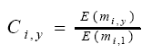
Figure 57. Equation. Mean of the estimate for 1993. Next, the ratios C1,y which are the ratios of E(m1,y) to E(m1,1) for each before year y, are calculated using the form of figure 58 and applied in figures 59-61.
Figure 58. Equation. Calculation for ratio before year y.
Figure 59. Equation. Ratio before year 1991.
Figure 60. Equation. Ratio before year 1992.
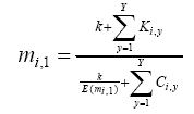
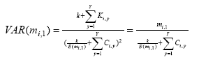
Figure 61. Equation. Ratio before year 1993. The next step is to calculate the expected crash counts mi,y on this site for each before year with their variance VAR(mi,y) using the equations in the figures below.
Figure 62. Equation. Expected crash counts.
Figure 63. Equation. Variance of the expected crash counts for year 1.
Figure 64. Equation. Expected crash counts.
Figure 65. Equation. Variance of expected crash counts. The application of these four expressions is shown in the equations in figures 66-71.
Figure 66. Equation. Application for 1991.
Figure 67. Equation. Application for variance 1991.
Figure 68. Equation. Application for 1992.
Figure 69. Equation. Application for variance 1992.
Figure 70. Equation. Application for 1993.
Figure 71. Equation. Application for variance for 1993. These results are summarized in table 38. Table 38. Estimation results for the before years.
Figure 72. Equation. Computation of E(m1,1995). Prediction of My+1, My+2,... My+Z for the After PeriodThe next step is to use the crash estimation model from figure 56 to compute the mean of the expected would-have-been crash frequency for the after period years. That is, even though Virginia changed from a differential to a uniform limit in 1994, there question remains of "what would the mean of the expected crash frequency have been had Virginia not changed its speed limit policy." Computation of these E(m1,y) values for the after period, as shown in figure 72 and 73, answers this question.
Figure 73. Equation. Computation of E(m1,1996). This process is repeated for the 1997 and 1999 years. One then computes the ratio Ci,y using figure 60, as illustrated in figures 74 and 75.
Figure 74. Equation. Computation of C1,1995.
Figure 75. Equation. Computation of C1,1996. Finally, figures 76 and 77 allow one to predict the would-have-been expected crash frequencies for the after years. Application of these methods is shown in figures 78-81.
Figure 76. Expected crash counts, year y.
Figure 77. Variance of expected crash counts, year y.
Figure 78. Equation. Expected crash counts, year 1995.
Figure 79. Variance of expected crash counts, year 1995.
Figure 80. Expected crash counts, year 1996.
Figure 81. Variance of expected crash counts, year 1996. These results are summarized in table 39. Table 39. Prediction results for the after years.
aKi,y: The actual after crashes for year y. Evaluation of Safety Effects of Changing the Speed Limit for This Particular SiteEvaluation of Safety Effects of Changing the Speed Limit for This Particular Site The effect of the treatment (that is, changing from a differential speed limit to a uniform speed limit) is determined by comparing the actual after crashes Ki,y with the predicted after crashes mi,y for each year of the after period. The cumulative differences, shaded in table 40, are computed by applying the equations in figures 82-84.
Figure 82. Equation. Total would-have-been crashes for a particular site.
Figure 83. Equation. Total actual crashes for a particular site.
Figure 84. Equation. Safety impact for a particular site. Table 40. Evaluation of the treatment for the example site.
An interpretation of table 40 is that, over the 4-year after period, the actual number of crashes at this site was 5.76 less than the predicted number of crashes that would have resulted had there been no change in the speed limit. Alternatively, the investigator could use the equation in figure 85 to indicate that the speed limit change decreased crashes by approximately 16 percent at the site, since the ratio of the actual crashes to "would-have-been crashes had no change occurred" is 0.84.
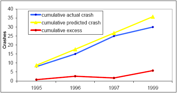
Figure 85. Equation. Ratio of actual to would-have-been crashes. The investigator can graphically portray these cumulative differences as shown in figure 86.
Figure 86. Chart. Cumulative differences, by year, at the example site. Evaluation of Safety Effects of Changing the Speed Limit for All SitesThe example shown above has been applied to only one particular site, but realistically a researcher would apply these concepts to all sites (e.g., in Virginia, 266 sites). Thus, using similar computations from all 266 sites, the investigator compares (a) the actual after crashes for the after period 1995 through 1999 that resulted under the uniform speed limit imposed in 1994, and (b) the would-have-been crashes for the after period 1995 through 1999 that would have resulted had the speed limit not been changed in 1994. Two basic performance measures, the reduction in the expected number of crashes (δ) and the index of effectiveness (θ), are computed and tested for statistical significance. The equations in figures 87-88 compute, respectively, the would-have-been crashes (those that would have occurred had no changes taken place) and the actual crashes that did occur. Since the equation in figure 89 shows that the actual number of crashes (λ) is larger than these wouldhave- been crashes (Π), the negative value of δ suggests that the speed limit change had an adverse impact on safety, and it would have been better not to make the change. This statement, however, needs to be tested for statistical significance.
Figure 87. Total would-have-been crashes.
Figure 88. Total actual crashes.
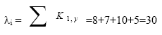
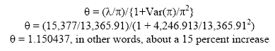
Figure 89. Safety impact. To determine statistical significance, the starting point is the variance as calculated in figure 92. The term ΣVar(Πi) is obtained by summing the values of VAR(m1,y) for each site and each year. Thus, the italicized values shown in the sixth column of table 40 (e.g., 2.39, 2.48, 2.57, and 2.58) would be computed for each site and for each year, and with 266 sites and 4 years of data, the 1,064 values of VAR(m1,y) are summed to equal 4,246.913. Because of statistical properties appropriate to the Poisson distribution, the summation of the λi values are equivalent to the variance of these values, which is 15,377 as tabulated in figure 89 above. These two items are used in figure 90 below to obtain Var(δ), which intuitively may be described as the variation associated with the difference between would-have-been crashes and actual crashes.
Figure 90. Variance of the difference between would-have-been crashes and actual crashes. The standard deviation is thus the square root of this variance in figure 91, such that:
Figure 91. Standard deviation of the difference between would-have-been crashes and actual crashes. Empirical confidence bounds are thus δ ± 2σ(δ) or -2011 ± 2(140). Computation of the index of effectiveness is accomplished via the equation below as:
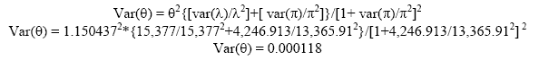
Figure 92. Equation. Computation of the index of effectiveness. The variance of θ is given below as:
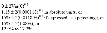
Figure 93. Equation. Variance of θ. The empirical confidence bounds are shown below:
Figure 94. Equation. Empirical confidence bounds. Thus, the change from DSL to USL in Virginia increased the number of crashes by about 15 percent, with the full response being that this 15 percent is not a perfect estimator but instead should be given as a range, such that the increase was between approximately 12.9 percent and 17.2 percent according to this application of the empirical Bayes method. Assuming all the other factors remained constant except for the change of speed limit from differential to uniform, therefore, the value of θ being greater than 1.0 means that the change had an adverse impact on safety, as reflected in the number of crashes on rural interstates in Virginia.
|
||||||||||||||||||||||||||||||||||||||||||||||||||||||||||||||||||||||||||||||||||||||||||||||||||||||||||||||||||||||||||||||||||||||||||||||||||||||||||||||||||||||||||||||||||||||||||||||||||