• Federal Highway Administration >
• Publications >
• Research Publications >
• 05048 >
• 7.Cfm >
• Safety Evaluation of Red-Light Cameras

Safety Evaluation of Red-Light Cameras

PDF files can be viewed with the Acrobat® Reader®

VII. Methodology for National, MultiJurisdiction Study

The experimental design for the national study was based on the study questions identified by the oversight panel, the noted issue-related findings from the literature review, the findings from the jurisdiction interviews, and the initial Phase I Scope of Work (SOW). Following is a list of factors, taken verbatim from the SOW, followed by a summary of the project team recommendation for consideration, which were incorporated in the final evaluation plan:

• Sample size requirements-How many treated sites (number of signalized intersections equipped with red-light cameras) are required?

  Recommendation 1: In the proposed experimental plan, the project provided sample size estimates based on assumptions of crash counts and safety effects. However, the project team believed that it may be more important to ask, "What can be achieved, that is, what effects can be detected and at what significance levels, with the data that are likely to be available?" These estimates were also provided.

• How many other types of sites (comparison or reference sites) are required to distinguish between what is the effect of the treatment and what is the effect of other factors such as changes in traffic flow, weather, and police reporting practices that may have also changed from the "before" to the "after" period? In other words, what technique will be used to estimate the number, severity, and types of crashes that could have occurred without the improvement?

  Recommendation 2: The multivariate empirical Bayes (EB) procedure was proposed for accounting for effects due to regression to the mean, traffic volume changes, and changes in other factors during the analysis period.⁽⁴⁾ In this methodology, the comparison group is used as a reference group for estimating annual adjustments for the safety performance functions that are key to the method. The number of crashes in the reference group needs to be large enough for this purpose. It was estimated, based on experience and on guidelines in Harwood et al. (2000), that 100 crashes per year for each crash type would be required.⁽²⁴⁾

• Spillover effect-There may be a large spillover effect of camera enforcement to intersections in the same community that are not equipped with cameras. The automated enforcement may provide general deterrence against red-light violations and crashes with effects not limited to specific intersections with cameras.

  Recommendation 3: The project team proposed that (a) this spillover effect be estimated separately from the specific deterrence effect and that it be related, if possible, to the proximity of a noncamera equipped intersection to an RLC site and (b) that untreated signalized intersections in the same community not be used as comparison sites to control for crash trends between the before and after periods. It was felt that these sites may be from neighboring communities or may be unsignalized intersections in the same jurisdiction. The use of signalized intersections from other communities raised issues of differences in crash-reporting practices between cities so the unsignalized intersection option was preferable. However, it was anticipated that the use of unsignalized intersections as the comparison group would make the study somewhat more difficult due to the fact that while the major cities interviewed tend to have detailed traffic count data on signalized intersections, not all have an abundance of data on unsignalized intersections.

• Types of crashes-It is desirable to obtain data that contain sufficient detail to identify crashes that were specifically red-light-running events. If it is not possible to categorize crashes specifically as red-light-running events, then the contractor should attempt to define red-light-running crashes as best as possible, given the data available. In addition, obtaining statistics for rear end crashes is necessary because they might increase under RLC enforcement due to increased driver compliance with stopping at red lights.

  Recommendation 4: Given the quality of available databases and that a retrospective study was required, it was felt that it would be impossible to achieve the desired goal of estimating the effects for crashes that were specifically red-light-running events. However, the project team believed that there are reasonable surrogates and proposed that, as a minimum, effects be estimated for left-turn opposed, right angle from adjacent approaches and, if possible, crashes in which a driver was charged for a red-light violation. Effects so estimated could be deemed to be conservative. It was also proposed that the effects on rear end crashes be separately estimated and that an assessment be undertaken of the net effects on crashes by considering the relative severities of the different crash types affected.

• Selection bias-The accident history of an intersection during the "before" period is an important clue to what would have been its safety performance during the "after" period. However, that same accident history may also be one of the reasons that that particular intersection was selected for treatment. This factor makes prediction of safety performance during the "after" period subject to bias called "regression to the mean" (RTM). In addition, the RTM bias may be present even if locations were not selected because of an abnormally high or unusually low rate of crashes.

  Recommendation 5: Substantial evidence of this bias was found in previous evaluations. The interviews also substantiated that virtually all cities use "high crash counts" as a factor in choosing the RLC locations (as would be expected and logical). Therefore it was deemed critical that regression to the mean be properly accounted for using the most advanced state of the art methodology. To this end, in Recommendation (2), the EB methodology was proposed; this methodology has other attractive features, e.g., the fact that it mitigates the difficulties in more traditional methods of identifying a comparison group for accounting for regression to the mean.

• Evaluation periods-The adoption of RLC enforcement is relatively recent in the United States; therefore, "after" periods will be short in most cases. The contractor should design a research study that will obtain as much "after" data as possible.

  Recommendation 6: Naturally, the research study should be designed to obtain as much "after" period data as possible. At the same time the study should ensure that the after period is at least one year long and that it ends at a time when it is certain that all crashes occurring have entered the database. On a related issue, the ability to detect an effect also depends on the before period crash count. Fortunately, the EB methodology is such that much longer before periods can be used than the period of two to four years employed in conventional before-and-after comparisons. Unfortunately, the available "before" data in cities is not as extensive as would be the case for State-controlled rural roads. Of the 15 cities interviewed, two have virtually no before-period data, three have 2 years, five have 3-4 years, and three have more than 5 years. The remaining two did not know how many years of data were available. Thus, two-thirds have 3 years or more.

The remainder of this section presents details of the design on the basis of these recommendations and data available in the jurisdictions interviewed.

Study Design Details

A detailed study design was proposed to the project oversight panel. The panel approved this plan after limited modification. The following text describes the design as ultimately implemented by the project team.

Basic Objectives and Main Analytical Requirements

The basic objective was to estimate the change in target crashes. Following is a list of possible target crash types:

• Right-angle (side impact).
• Left-turn (two vehicles turning).
• Left-turn (one vehicle oncoming).
• Rear end (straight ahead).
• Rear end (while turning).
• Other such as crashes specifically identified as red-light-running.

These were estimated separately for two groups of sites:

• Sites where cameras are used (specific deterrence effects).
• Signalized intersections without cameras at various levels of proximity to the treatment sites.

The preparation of a study design entailed both the preparation of a data collection plan and an analysis plan. The analytical requirements to provide the desired estimates drove the data collection needs.

The analysis examined the safety effect of red-light-camera enforcement to provide insights into a number of issues, within the confines of available data. The data collection plan, discussed later in this report, provided insights into the capacity of the available data to address these issues. Meeting the objectives and addressing the key issues placed the following list of special requirements on the data collection and analysis tasks:

• Select a large enough sample size to detect, with statistical significance, what may be small changes in safety for some crash types.
• Select carefully comparison sites or cities to ensure that safety at these sites is unlikely to be affected by the RLC installations.
• Account properly for traffic volume changes.
• Pool data from several jurisdictions to improve reliability of results and facilitate broader applicability of research products.

Overview of the General Evaluation Methodology

The general analysis methodology used is different from those used in the past, benefiting from significant advances made in the past 10 years in the methodology for the conduct of observational before-and-after studies, which culminated in a landmark book by Hauer.⁽⁴⁾ That book also provides guidance on study design elements such as size and selection criteria for treatment and comparison groups and the pooling of data from diverse sources. All these are crucial elements in successfully conducting a study to obtain results that will have wide applicability.

The evaluation considered the issues identified earlier on the basis of panel input and the literature review and survey to the extent that is practical. The inclusion of a variable in the analysis was ultimately resolved on the basis of whether relevant data could be obtained within the confines of the project, and whether obtainable sample sizes and the variation in levels of a variable were sufficiently large to isolate its effects (if any).

The methodologies documented by Hauer range from simple before-and-after comparisons to the more powerful EB methodology.⁽⁴⁾ The team proposed that the latter approach be pursued in seeking to overcome the difficulties associated with conventional before-and-after comparisons, while providing a fresh approach to overcome the limitations of previous evaluations of red-light cameras. Specifically, the analysis would:

• Properly account for regression to the mean.
• Overcome the difficulties of using crash rates in normalizing for volume differences between the before-and-after periods.
• Reduce the level of uncertainty in the estimates of safety effect.
• Provide a foundation for developing guidelines for estimating the likely safety consequences of contemplated RLC installation.
• Properly account for differences in crash experience and reporting practice in amalgamating data and results from diverse jurisdictions.
• Avoid the difficulties of conventional treatment-comparison experimental designs caused by possible spillover and/or migration effects to natural comparison groups.

In the EB approach, the change in safety for a given crash type at an RLC intersection is given by equation 1:

(1)

where π is the expected number of crashes that would have occurred in the after period without the cameras and λ is the number of reported crashes in the after period.

In estimating π, the effects of regression to the mean and changes in traffic volume were explicitly accounted for using safety performance functions (SPFs) relating crashes of different types and severities to traffic flow and other relevant factors for each jurisdiction based on a reference group of signalized intersections without RLCs. Annual SPF multipliers were calibrated to account for the temporal effects on safety of variation in weather, demography, crash reporting and so on. Because of the possibility of spillover effects to the reference group of signalized intersections, it was decided to estimate the annual multipliers for the period after the first RLC installation from the trend in annual multipliers of SPFs calibrated for a comparison group consisting of unsignalized intersections in the jurisdiction.

In estimating the SPFs a parameter k, which is a constant for a given model, is iteratively estimated with the use of a maximum likelihood procedure. (In that process, a negative binomial distributed error structure is assumed with k being the dispersion parameter of this distribution; the estimated value of k is the one that maximizes the likelihood of observing the crash counts, given the calibrated SPF.) See Hauer for more detail.⁽⁴⁾

Empirical Bayes Before-and-After Evaluation Example

An illustration of the EB before-and-after evaluation methodology is provided next. Full theoretical details can be found in Hauer.⁽⁴⁾ This example of the evaluation methodology is applied at a site and aggregate level. Note that the data presented are for illustrative purposes only, and do not represent data collected in this study.

Data and SPFs:

Consider an intersection at which RLC was implemented in September 2000. Refer to this as site (i). Suppose it is desired to estimate the effect of RLC on right angle injury crashes at this site.

Suppose the SPF for right angle injury crashes for a given year y in the before period for this jurisdiction is:

(2)

where "_y is the calibrated multiplier for this jurisdiction for a given year using the recalibration procedure, and MAJAADT_y and MINAADT_y are respectively the major and minor road entering average annual daily traffic (AADT) in year y.

For this illustrative example, it is assumed that the recalibration process has been completed, and that the values of "_y are as given in table 6. That process also calibrated a value of 1.44 for the negative binomial distribution overdispersion parameter k that is used in the EB procedure. Crashes are available from 1996-2001 as shown in table 2. For illustrative purposes, assume that the yearly entering AADTs were either all available or some were estimated using a procedure in Lord.⁽²⁵⁾ The AADTs are also shown in table 2.

Effect for Site (i):

The calculations in table 2 are based on the methodology in Hauer.⁽⁴⁾ They pertain to a single site (i) for which the results show that p(i) = 4.384 right angle injury crashes are expected in the after-period without treatment. Four such crashes (l(i)) were recorded.

The crash modification factor for this one site is, from Hauer:⁽⁴⁾

(3)

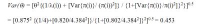
It means that the point estimate of the crash reduction is 100(1- 0.875) = 12.5%.

Table 2 shows the AADTs for the EB evaluation example.

Table 2. Summary of results for right-angle injury crashes at site (i).

The standard deviation of q (from Hauer) is given by:⁽⁴⁾

(4)

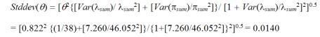
Aggregate effects over several sites:

Results for a single site will tend to be meaningless and almost certainly lack reasonable statistical significance. To aggregate results over several sites, the procedure is to simply add their individual values of the l(i), p(i), and Var{p(i)}over all sites and replace these values in the equations with their respective sums, l_sum, p_sum, and Var{p_sum)}.

For illustration, five sites with various lengths of before and after periods are added to the analysis. Assume that the observed number of crashes, l(i), the expected number of crashes without treatment, p(i), and its variance Var{p(i)} have been calculated and are given in table 3. In this example one site (Site 4) experienced more crashes in the after period than expected.

The crash modification factor for the five sites is, therefore:

(5)

This means that the point estimate of the composite crash reduction percentage of 100(1-0.822) = 17.8 percent.

The standard deviation of this composite q is:

(6)

By including more sites in the analysis, some with relatively long after periods, q has been estimated more accurately with a standard deviation of 0.140 compared to 0.453 using only one site with a short after period. Table 3 shows the composite effect at five sites, for illustration.

Table 3. The composite effect over several sites (for illustration).

Data Collection Plan

Based on the requirements for the methodology described, the project team then developed a data collection plan. The first aspect of the plan was the choice of jurisdictions to include in the study. In the following description, this choice was based on sample size needs and the data available in each jurisdiction. The second aspect of the plan involved the specification of data variables to be collected.

Choice of Jurisdictions

Evaluation Study Sample Size Estimation:

When planning a before-and-after safety evaluation study it is vital to ensure that enough data are included such that the expected change in safety can be statistically detected. Even though in the planning stage the expected change in safety is not known, it is still possible to make a rough determination of how many sites are required based on the best available information about the expected change in safety. Alternatively, one could estimate, for the number of available sites, the change in safety that can be statistically detected. For a detailed explanation of sample size considerations, as well as estimation methods, see chapter 9 of Hauer.⁽⁴⁾ The sample size analysis presented in this section addressed two cases: 1) how large a sample is required to detect statistically an expected change in safety and 2) what changes in safety can be detected with likely available sample sizes. The focus is on detecting effects at the treatment sites. It was assumed (and was later verified) that the number of noncamera equipped signalized intersections will be sufficiently large that spillover effects, if present, will be detected.

Case 1-Sample Size Required to Detect an Expected Change in Safety:

For this analysis, it was assumed that a conventional before-and-after study with comparison group design would be used, because available sample size estimation methods are based on this assumption. The sample sizes estimates so provided would be conservative in that EB methodology proposed would require fewer sites. To facilitate the analysis, it was also assumed that the number of signalized reference sites is equal to the number of treatment sites. This assumption was very conservative, because it was later decided to attempt to collect data on three signalized reference sites for each treatment site to better explore the spillover effect.

The statistical accuracy attainable for a given sample size is described by the standard deviations of the estimated percentage change in safety. From this, one can estimate P-values for various sample sizes and expected change in safety for a given crash history. A set of such calculations is shown in table 8 based on assumptions of 20 crashes/site-year of which 3.5 are right angle crashes and 12.0 are rear end crashes, 3 years of "before" crash counts, 1.5 years of "after" period crash counts. The crash rates are estimated as an average of published data for RLC sites in Charlotte, NC, and Howard County, MD. The calculations are based on methodology in Hauer and a spreadsheet on his Web site, http://www.roadsafetyresearch.com.⁽⁴⁾

Table 4. P-values for various sample sizes and expected changes in safety.*

*Based on 3.5 right angle and 12.0 rear end crashes/site-year, and before and after periods of 3 and 1.5 years respectively.

The shaded cells in table 8 indicate where P-values of at least 0.10 are attainable. Thus, for example, if the sample contains 20 treated sites, and a 30-percent reduction in the number of right-angle crashes is expected because of the RLC installation, one may expect to obtain a statistically significant result at the 10 percent level (P = 0.05). With 60 treated sites, if there is a 20-percent increase in the number of rear end crashes, one may not expect a statistically significant result at the 5 percent level (P > 0.10); however, that result would be significant at the 15 percent level.

Case 2- Safety Change Detectable with Likely Available Sample Sizes:

On the basis of preliminary crash data available early in the study, an estimate was made of the maximum percentage change in crash frequency that could be statistically detectable at 5-percent and 10-percent significance levels. Estimates were prepared for a variety of severity and impact types and for four representative jurisdictions from the survey. Because it was likely that additional data would become available as the study proceeded, it was felt that these estimates could be regarded as conservative. The estimates were also conservative based on other considerations mentioned below.

The crash rate assumptions in table 5 were used for this exercise. They were based on published data from RLC installation sites in Howard County, MD (HC), and Charlotte, NC (CH), and on typical severity ratios indicating that about 35 percent of all crashes at signalized intersections involve injuries.

Table 5. After period crash rate assumptions.

Tables 6 and 7 show, for each crash type, an estimate of the number of intersection years of after-period crash data for treatment sites in each of several jurisdictions and for 2 groups of jurisdictions. Separate parts of the table are presented for right-angle and rear end crash effects. For the two crash rate assumptions it shows the maximum percentage change in crash frequency that would be statistically detectable at 5 percent and 10 percent levels of significance for both crash rate assumptions. (For Howard County and Charlotte, only their respective crash rates from table 6 are used.) Only jurisdictions with 10 or more intersection years in the after period were considered as feasible for this analysis. Assuming that some sort of a national estimate would be useful and could be obtained through amalgamation of the results over several jurisdictions, which is certainly possible for injury crashes at least, calculations were also shown for two groups of jurisdictions:

• All jurisdictions listed
• The "top seven" which includes jurisdictions for which significant effects are likely for all crash severities (Howard County, Baltimore, Charlotte, San Diego, San Francisco, Montgomery County, and El Cajon City) but excludes New York City because its data were found to be unsuitable for use in this study. These "top seven" were ultimately included in the study.

This presentation allowed for various options for deciding on the size of the planned retrospective study; nevertheless, it was felt that consideration must also be given to the ease or difficulty of obtaining quality data from each jurisdiction (which is why New York City was ultimately excluded).

Table 6. Sample analysis for right-angle crash effects.

^* Assumes a decrease in right-angle crashes and an increase in rear end crashes.

^a Group 1 includes Howard County, Baltimore, Charlotte, San Diego, San Francisco, Montgomery County and El Cajon City.

Table 7. Sample analysis for rear end crash effects.

^* Assumes a decrease in right-angle crashes and an increase in rear end crashes.

^1a Group 1 includes Howard County, Baltimore, Charlotte, San Diego, San Francisco, Montgomery County and El Cajon City.

Sample Design Conclusions:

Judgments on the likelihood of detecting significant effects assume that there is, in fact, an effect on crashes. If an effect does not exist, of course, no effect will be statistically detectable. Table 8 presents the authors' best judgment during the sample design stage on the likelihood of detecting (at the 10-percent level) safety effects expected on the basis of the literature review, which revealed that it is not unreasonable to expect effects on the order of a 25-percent decrease in right-angle crashes and a 30-percent increase in rear-end crashes. Even so, for reasons explained earlier, these judgments were based on results that are likely to be conservative.

Table 8. Best judgment on possibility of detecting safety effects.

U = significant results may be obtained W = significant results may not be obtained.

Selection of Study Jurisdictions

As noted, the Us in table 8 were based on one criteria for inclusion in a study of RLC effects-the available crash data. However, there were other criteria that needed to be considered-the availability and quality of the other data. Table 9 summarizes these crash-related findings from table 8, along with information on other data extracted from the interview forms. While a variety of information was captured in the interview, because of both study needs such as traffic flow data and the high-priority questions of interest, emphasis was placed on the presence of data on yellow interval changes, traffic flows at signalized and unsignalized intersections, the level of publicity campaign (to attempt to get a range of levels), and the type of signing. Note that the level of the publicity campaign was a project staff judgment based on the jurisdiction's response to the initial telephone questionnaire discussion concerning public information. In the questionnaire, the three levels were given the following definitions:

• High-A major planned public information campaign including components such as the FHWA public information program, combined PI efforts with other departments in the jurisdiction (e.g., local health department), and television spots.
• Medium-Moderate public information program with limited expenditures, but good coverage of the RLC effort by news media.
• Limited-Limited public information program with media coverage only from interviews or press conferences, or both.

Table 9 shows 3 categories of the authors' judgment of the best cities based on these data variables. Howard County, MD, was judged the best overall, shown with bold italics. The second group of cities (in some order of preference) are those in italics-Baltimore, MD, Charlotte, NC, San Diego, CA, San Francisco, CA, Montgomery County, MD, and El Cajon City, CA. Each has some shortcomings, either in crash sample size or other data. For example, Baltimore has limited traffic count data, and El Cajon City's crash data require further investigation. The remaining cities had serious problems either in crash counts or other data or in the size of the sample.

Table 9. Best judgment on sites to use based on crash and non-crash data available.

Significant Crash Types: ARA-All right-angle; IRA-Injury right-angle; ARE-All rear end; IRE-Injury rear end

Signal Data Available: YI-Yellow interval (length and changes); ARI-All-red interval (presence and changes); CL-Cycle length, SC-Signal coordination

Traffic Data Available: FTC-Full traffic counts (i.e., regular program of traffic counts for all signalized intersections); LTC-Limited traffic counts (some intersections, or only as requested); No-no traffic counts; UITC-Unsignalized intersection traffic counts

Public Information: HPI-High public information campaign; MPI-Medium public information campaign; LPI-Limited public information campaign; SI-Warning signs at intersections; SO-Warning signs at other locations (e.g., edge of town or corridor); SB-Warning signs at both intersection approaches and other locations

Note that, as indicated earlier, New York City, the site with the largest crash sample, fell into the infeasible group because of the lack of traffic count data. New York City was also considered different from other U.S. cities by an RLR expert outside the project team because of its size, the number of intersections, the small proportion of intersections that are treated, the possible dilution of any publicity campaign, high tourism, and other factors.

As can be seen, three of the cities appeared superior to the other four cities-Howard County and Baltimore, MD, and Charlotte, NC. While a multijurisdictional study could be done with just these three cities, the project team did not recommend that because the sample size of jurisdictions would be small, two are in Maryland, and all three are eastern cities.

Data Collection Requirements

It was recommended that, for any installation a minimum of 2 years of before-period and 1 year of after-period information should be available and that, ideally, at least 3 years of crash data be required for each of these periods. As found later in the actual data collection, all sites in all jurisdictions had 4 to 9 years of before-period data, with an average before-period of 6 years. The length of the after period data varied from less than 1 year (in approximately 8 percent of the sites) to 5 years, with an average after-period of approximately 2.76 years for all sites.

Crash data for the same years were also required for a reference group of locations, similar to the RLC locations, except that these were not equipped with RLCs. These sites were to be used in the recalibration of safety performance functions and to investigate possible spillover effects. Because the reference group was to be used both for this SPF recalibration and to study the distance-of-influence issue, a later decision was made to attempt to identify three reference-group signalized intersections for each treated intersection in a jurisdiction. To account for time trends between the before-and after-periods, crash data also were collected from a comparison group of approximately 50 unsignalized intersections in each jurisdiction.

Table 10 lists the basic data items originally proposed for collection. As will be described in the later section concerning data collection, modifications were made to this listing based on available data and funding issues.

Table 10. Data items required.

Previous | Table of Contents | Next