• Federal Highway Administration >
• Publications >
• Research Publications >
• 08034 >
• 02.Cfm >
• Wildlife-Vehicle Collision Reduction Study: Report To Congress

Wildlife-Vehicle Collision Reduction Study: Report To Congress

PDF files can be viewed with the Acrobat® Reader®

Chapter 2. Causes and Characteristics of Wildlife-Vehicle Collisions

The primary method of investigating the causes and characteristics associated with WVCs is to analyze data on previous collisions. This chapter provides a summary of current knowledge about WVCs, based on information from the literature and an update from national crash databases. After discussing data sources and evaluation methods, this chapter investigates the following characteristics of WVCs:

• Total magnitude.

• Growth rate.

• Temporal distribution by:

  • Time of day.

  • Time of year.

• Severity of human injuries and fatalities.

• Roadway facility type.

• Traffic density and speed.

• Weather conditions.

• Animal species.

• Landscape adjacent to roads.

• Number of vehicles involved.

• Deer population density.

• Driver characteristics.

Data Sources

Numbers and factors related to WVCs have been reported extensively in the literature. Possibly the most commonly quoted statistic is that there are over one million WVCs with large animals annually in the United States. This number originally comes from a survey of states completed by Romin and Bissonette.⁽³⁾ States responded to this survey with a mix of crash record numbers, carcass counts, and estimates. Approximately 500,000 DVCs were reported by 35 states. Conover and others estimated that DVCs are underestimated by at least 50 percent, so most researchers increase this number to one million or more to include the missing states and unreported crashes.⁽⁴⁾

There are three common sources of data for WVCs: carcass counts, the insurance industry, and police-reported crashes. The first source, carcass counts, includes counts of dead animals on the side of the roadway that likely died from collisions with a vehicle. Sometimes these data include more detail than just the species (e.g., sex, age, size, etc.). Unlike the two other sources discussed below, carcass counts are not always focused on safety and can include smaller animals since conservation concerns are also a reason to collect carcass data. This source of data may be sufficient for corridor or regional studies, but the lack of consistency in reporting methods limits evaluation on a statewide or national level. However, it is often thought that carcass counts are the most comprehensive data available since the following two sources tend to underreport the total number of WVCs.

Another source of information on WVCs is data from the insurance industry, which is based on reported claims. Claims typically relate to major damage, and major damage is typically associated with relatively large animals (e.g., deer size and up). State Farm Insurance estimated the number of claims for collisions with deer, elk, and moose and then estimated the total number nationally based on the company's proportion of market share of insurance policies.⁽⁵⁾ This estimate is questionable. The number may underreport total collisions, since it only includes vehicles with comprehensive insurance; accidents with uninsured vehicles are not reported to the insurance industry. On the other hand, it could be overestimating crashes, since people may be likely to say they hit a deer when they actually hit something else in an attempt to keep their insurance rates low. As shown in figure 1, there are approximately one million WVC insurance claims annually (years are shown as fiscal years, July 1–June 30). This source of data typically does not contain detailed information about each crash.

Figure 1. Graph. Annual WVCs estimated by insurance industry.⁽⁵⁾

The third source of WVC information is police reports of total crashes of all types (including WVCs). These reports are more effective for analyzing data nationally, because there is more consistency in their collection. The transportation industry expends considerable effort collecting and cleaning up these data for accurate analysis. However, this data set also has its limitations. These data only include crashes on public roads. In addition, these reports only include data for accidents that incurred a certain level of damage to the vehicle (each state has its own reporting threshold). Finally, the data may not include information on animal species, because these reports are focused on safety in general and are not specific to WVCs. In fact, the crashes may only be categorized as AVCs (not separating domestic and wild animals). Three national police report-based datasets were used in this review as described below.

National Crash Databases

Each state maintains its own database of crash records with different reporting thresholds, different variables describing the contributing factors, and different database structures. WVCs were analyzed from three sources:

• Fatal Accident Reporting System (FARS) includes all crashes nationally that involve a human fatality. The data from this system are likely the most consistent nationally since more detail and effort goes into reporting a fatal crash. However, the dataset is small with typically fewer than 200 AVC fatal crashes annually. From 2001 to 2005, an average of 38,493 fatal crashes occurred.⁽²⁾ Hence AVCs represent roughly 0.5 percent of fatal crashes.

• The Highway Safety Information System (HSIS) includes all reported crashes from Washington, California, Illinois, Maine, Michigan, Minnesota, North Carolina, Ohio, and Utah. This is a useful source of data since some of these states report more detail on the species of animal involved in a crash. Although it contains all crashes reported, it is only for the selected states.

• The General Estimates System (GES) is a true national sample. A small random sample of police accident reports is collected from each sampling unit. A sampling unit contains one or more police jurisdictions. The values from these police reports are aggregated up to determine national estimates. Although the collection methods are rigorous to ensure randomness, this is still only a sample of all crashes, so these are estimates of national values, not true national values.

Throughout the rest of this chapter, numbers are reported from each of these three datasets. General issues and methods for analyzing these datasets are discussed here. It should be noted that national figures are analytically attractive because there is a much larger dataset, but they may mask significant differences in WVCs between local areas.

Fatal Accident Reporting System

Fatal Accident Reporting System (FARS) data include those crashes where at least one person died within 30 days of the collision from collision-related injury. Data were collected from 2001 to 2005. AVCs were identified when a crash's "first harmful event" was an animal. Note that for these events, the "most harmful event" was not always an animal. Data were downloaded from the FARS Web site (http://www-fars.nhtsa.dot.gov/) (accessed November 27, 2006). The first harmful event is the first event during a crash that causes injury or property damage. The most harmful event causes the most damage and is not always the same as the first harmful event.

Highway Safety Information System

HSIS data contain police-reported accidents for Washington, California, Illinois, Maine, Michigan, Minnesota, North Carolina, Ohio, and Utah. HSIS was developed and is maintained by FHWA. Information can be found at http://www.hsisinfo.org (accessed January 24, 2007). This database includes all police-reported crashes for these states; therefore, it has a larger sample than the random sample in the GES dataset, but it does not contain data beyond these states. A strength of this dataset is that some of the detail collected by individual states is maintained. For example, Maine divides its AVCs into deer, bear, moose, and other.

HSIS states have different data availability. The most recent 5 years of data from each state were analyzed (table 1). Also shown in table 1 are the reporting thresholds for each state.

The manner in which animals are categorized also varies between states (table 1). Some states simply have a single general category of "animal" for all AVCs. One category for all animals is similar to the GES and FARS animal categorization, which can include domestic animals. When reporting on HSIS data as a whole, domestic animals were excluded (unless otherwise stated) for those states that differentiated. As such, HSIS results refer to WVCs, even though some of the states may include domestic animals within their animal classification.

Crash data can sometimes be misleading when a clear and detailed explanation of the reported value is not provided. For example, from the same source of data one could state that there were 100 crashes, or that 200 vehicles were involved in a crash (i.e., there were 100 crashes, each involving two vehicles). In this report, unless otherwise stated, crash numbers refer to number of crashes (not number of vehicles or people). When referencing the vehicle attribute, it refers to the vehicle that struck the animal (almost all crashes were single-vehicle crashes). When referencing the person attributes, it refers to the driver of that vehicle.

To compare data from states with vastly different numbers of collisions (range = 176,793 to 890,215), proportions of collisions were compared instead of raw numbers. Further, rather than using the sum of all collisions with certain characteristics (which would bias the total towards states with more collisions), the proportion of collisions within each state was summed and divided by the number of states.

General Estimates System

GES is a stratified random sample. There are actually two strata. The first stratum is geographic. There are four regions (Northeast, Midwest, South, and West) that are further categorized into 1,195 primary sampling units, each containing one or more police jurisdictions. Within these geographic areas, crash reports are sampled randomly. The second stratum is crash type (mostly in terms of severity). Crash types are divided into the following categories:

• An occupant of a vehicle that was towed after the collision is killed or severely injured—no medium or heavy trucks.

• An occupant of a vehicle that was towed after the collision is injured—no medium or heavy trucks.

• A passenger vehicle is towed after the collision (no fatalities or injuries)—no medium or heavy trucks.

• A medium or heavy truck that resulted in a vehicle being towed or an injury report.

• No vehicles were medium or heavy trucks, no vehicles were towed, and at least one person was injured.

• No person was injured.

The total number of crash reports (including those not sampled) is also known for each geographic and crash type sampling unit. Based on these sampling units, rates are determined such that each crash record is given a weight that is an estimate of the number of crashes it represents. When comparing across the crash strata mentioned above or considering total AVC numbers, the weighting factors were used. Since these weighting factors have not been published for 2005, these numbers represent 2000–2004 data. When considering variables within the AVC subsample (e.g., time-of-day distributions), straight proportions were used assuming there were random samples across nonsampling unit variables. For these numbers, 2001–2005 GES data without weights were used. The assumption regarding these proportions was not validated. Future analysis should include the most recent available data and include the weighting factors. GES data were downloaded from ftp://ftp.nhtsa.dot.gov/ges/ (accessed January 24, 2007).

Total Vehicle Miles Traveled

Researchers collected data on vehicle miles traveled (VMT) for each state. This information, coupled with the crash data described above, allowed for determination of crash rates. These rates are expressed as crashes per million VMT unless otherwise stated. These values allow researchers to compare crashes both geographically and over time to see if there is an increase in the exposure rate. VMT files were downloaded from the U.S. Department of Transportation, Bureau of Transportation Statistics (BTS) Web site at http://www.bts.gov/ (accessed January 24, 2007). Annual national VMT were available through 2004.

Evaluation Methodologies

The goal of the remainder of this section is to summarize how WVCs (or AVCs when crash data could not be separated into domestic and wild animal) are unique from other crashes. It is difficult to normalize for all the secondary factors that may cause a certain distribution of WVCs for a given variable. The best method is to compare WVCs with non-WVCs. A proportional t-test or chi squared test can be completed to confirm a statistically significant difference. In the case of all reported differences, they were statistically significant.

Total Magnitude

Based on the HSIS data, Table 2 shows the WVCs for each of the eight states analyzed. The proportion of crashes that were WVCs in a given state ranged from 0.6 to 14.6 percent. The total number of WVCs in these eight states was 251,619 for a 5-year period (about 50,000 per year). Consider that these states comprise 16 percent of the total land area in the 50 United States and 22 percent of the rural VMT in 2004. Considering the HSIS data represent about one-fifth of the United States, the national number of reported crashes is likely to be around five times the amount reported in the HSIS states (i.e., 50,000 per year). Extrapolating the HSIS data would yield an estimate of about 250,000 WVCs per year in the United States.

GES estimates the national average of AVCs at 292,000 annually (2001–2004). This value represents 4.6 percent of all crashes annually. Based on FARS data, the total number of fatal crashes involving AVCs nationally averages 179 per year (2001–2005). From 2001 to 2005, an average of 38,493 fatal crashes occurred for all crash types.⁽²⁾ Hence AVCs represent, on average, less than 0.5 percent of all fatal crashes.

As mentioned previously, carcass counts have been extrapolated to a national estimate of over one million per year. Additionally, as shown previously in figure 1, the estimated number of insurance claims per year averages about one million. Table 3 summarizes the WVC counts from these various sources.

Marcoux conducted a survey in Michigan and found that of the people involved in a DVC, only 52 percent reported it to their insurance company.⁽⁶⁾ This finding implies that the estimated WVCs are underreported. The carcass counts are also not likely to include all WVCs, since they are extrapolated from a mix of reported collisions and carcass counts as well as from 35 to
50 states. Considering all of these figures and the previously discussed potential underreporting, the authors recommend the following two numbers be used when discussing the magnitude of WVCs with large animals:

• The total count of WVCs each year is between one and two million.

• The number of WVCs that are reported to police and have enough property damage to warrant tracking in crash databases (e.g., greater than $400–1,000 depending on the state) totals 300,000 per year.

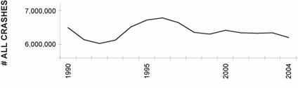
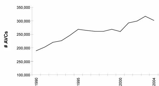
Keep in mind that each of these numbers represent WVCs with large animals since they are based on reported crashes or carcasses. The total magnitude of WVCs with small animals is likely much larger.

Is the Problem Growing?

Is the number of WVCs increasing or decreasing? A previous study of HSIS data found that WVCs increased 69 percent from 1985 to 1991.⁽⁷⁾

Since GES data are likely the best source of national numbers, trends were examined using this data source, extending back to 1990. As shown in figure 2 and figure 3, the number of all crashes is holding relatively steady at slightly above six million, while the number of AVCs is increasing. This increase could be due to a number of different factors discussed later in this chapter such as an increase in deer population and changes in traffic volumes and speeds.

To analyze WVC trends over time, three linear regression models were used, with the independent variable being the year and the dependent variable being either the total number of WVCs, the proportion of WVCs to total crashes, or the total crash rate. An important statistic is the t-statistic for the coefficient of the slope, which describes the relationship between the dependant and independent variables. If the t-statistic is greater than two, it can be confidently concluded (= 0.05 or 95 percent confidence) that the slope is not zero (i.e., the rate of WVCs changing through time). Statistically a linear regression line on the total annual AVCs shows an increasing slope of 6,769 AVCs per year (t = 7.8, R-squared = 0.81). In addition, the proportion of AVCs to total crashes has a positive slope of 0.11 percent per year (t = 9.4, R-squared = 0.86). Note that a higher R-squared value (which ranges from zero to one) indicates there is a linear relationship. An R-squared value of one results from a perfect linear relationship.

Figure 2. Graph. Total vehicle crashes.

Figure 3. Graph. Total AVCs (including wildlife and domestic animals).

To ensure that the increase in WVCs over time was not due only to increases in the amount of travel (i.e., VMT), the crash rate was investigated. Figure 4 shows the crash rates each year determined by dividing GES annual numbers by VMT. The linear regression of crash rate over time has a positive slope of 0.00072 crashes per million VMT per year (t = 2.2, R‑squared = 0.27). The linear relationship is weak as indicated by a low R-squared value. The t‑statistic shows that the crash rate increase is statistically significant.

Statistical analysis beyond linear regression models will be considered in future stages of this topic to further assess relationships.

Figure 4. Graph. Annual crash rate for AVCs (GES and VMT data).

Temporal Distributions

For some species, there are clearly certain times of the day and times of the year when WVCs occur more frequently. For large mammals, numerous studies have shown that WVCs occur more frequently in the morning (5–8 a.m.), the evening (4 p.m.–12 a.m.), in the fall (October and November), and in the spring (May–June).^(8,9,10) The peak in the spring is generally not as high as that in the fall. The daily peaks are typically explained by the fact that deer and other large animals are moving around dusk and dawn, which, combined with relatively high traffic volume in the early morning and late afternoon, results in a peak in collisions in the early morning and late afternoon and evening. The fall peak is typically explained as being related to mating season, migration, and hunting season, all of which cause animals to move around more.⁽¹¹⁾ The spring peak is explained by distribution of young and migration.

Figure 5 shows the annual AVC distribution for the three reported crash datasets. The HSIS- and GES-based AVC distributions are very similar in magnitude and shape. The FARS data do not have the sharp peak in AVCs observed in November in the other two datasets. Note that for the HSIS data most of the states followed the same basic trend. Five of the eight states had substantial peaks in proportion of AVCs in November, while two states ( California and Washington) had a larger peak in October and a smaller peak in November. Utah had the least overall difference in WVCs by time of year. All states except North Carolina and Utah had minor peaks in WVCs in spring, generally in June.

Figure 5. Graph. Annual distribution of AVCs.

Some HSIS states separated deer from other animals (WA, ME, IL, UT, and CA). For the "other animal" or domestic classifications the distribution is much more uniform throughout the year (figure 6).

Figure 6. Graph. Annual distribution for other/domestic animal-vehicle collisions in CA, WA, IL, ME, and UT (HSIS data).

Maine was the only HSIS state to list specific wild species other than deer. For Maine, the annual distributions for bear- and moose-vehicle collisions (figure 7) do not have the major peak in November like deer (note AVCs reported in figure 5 are primarily deer). Bear-vehicle collisions are fairly uniform in the summer and nonexistent in the winter during their hibernation period.

Figure 7. Graph. Annual distributions for moose and bear collisions in Maine (HSIS data).

Seasonal distributions appear to be somewhat dependent on specific geographic area. For example, in Teton County, Wyoming, WVCs were most frequent in summer months, especially in Grand Teton National Park, which has much higher traffic volumes in the summer.⁽¹²⁾ These numbers contrast sharply with the more regional trends presented in figure 5.

For time of day, the three data sources all show the expected peaks at early morning and evening (Error! Reference source not found.). Wildlife, especially deer, typically move around more at dusk and dawn.

Figure 8. Graph. Time-of-day distribution.

Severity

Williams and Wells looked at 147 fatal WVCs from nine different regions and found that the most common types were (1) a motorcyclist striking an animal and falling off the vehicle followed by (2) a passenger vehicle striking an animal, going off the road, and striking a fixed object or overturning. Safety measures (i.e., helmets and seat belts) were not used in
60–65 percent of the cases.⁽¹³⁾ Jones also reported most fatal crashes involved motorcycles.⁽¹⁴⁾ This conclusion was confirmed by the FARS data. On average, 30 percent of the fatal crashes involving animals also involved motorcycles. Conn and others investigated 22,498 emergency room visits where a motor vehicle collision with a large animal was identified as the cause.⁽¹⁵⁾
Of these, more than one-third (8,508) were people ages 15 to 24.

In general, WVCs are less severe than other crashes. Compared to all crashes, the datasets show the proportion of crashes involving human injury is much less for WVCs. GES-based estimates of crash severity over 5 years are shown in figure 9 and figure 10 for AVCs and all crashes, respectively. Almost all AVCs resulted in no human injury (95.4 percent). This figure is consistent with the HSIS data that show 92.3 percent of crashes resulted in no human injury. There was some variability in severity values between the HSIS states, likely due to the different reporting thresholds. California showed only 87.4 percent of DVCs resulted in no injury. GES estimated fatal crashes at 608 in a 5-year period, compared to 895 in the FARS data. However, the upper confidence interval of the GES data is 1,956 fatal crashes. Note that for all crashes in this same 5-year period, FARS shows 192,463 fatal crashes.

Figure 9. Graph. Severity distribution for AVCs (GES data).

Often collisions with moose and other larger animals are thought to be more fatal to humans than collisions with deer. In Newfoundland, Joyce and Mahoney found that among moose-vehicle collisions, 0.6 percent were fatal crashes and 26 percent were injury crashes.⁽⁸⁾

Figure 10. Graph. Severity distribution for all crashes (GES data).

From the HSIS data, domestic, livestock, and other animals had a slightly higher severity rate than WVCs, with 79.2 percent of crashes resulting in no human injury, which is lower than the 92.3 percent value for all AVCs, but still higher than the 68.3 percent value for all crashes. Moose-vehicle collisions from the Maine HSIS data show a severity profile more similar to that of all collisions (figure 11).

Figure 11. Graph. Severity distribution of moose-vehicle collisions in Maine (HSIS data).

Facility Type

Most studies that look at the types of roadways where WVCs occur report that they are most common on rural two-lane roads.⁽⁷⁾ However, these results should be used with caution since a large majority of highway miles are rural, two-lane roadways.

For the GES records with number of lanes and facility types, 89.7 percent of AVCs occurred on two-lane roads. In comparison, 52 percent of all crashes occur on two-lane roads (figure 12). This is not to say that upgrading all two-lane roads would reduce WVCs. Reilly and Green found that the upgrade from two to four lanes in constructing Interstate 75 in Michigan initially resulted in a 500 percent increase in DVCs.⁽¹⁶⁾ With time, the number of DVCs did steadily decrease. The initial increase could have been due to deer being unfamiliar with the new character of the roadway.

Figure 12. Graph. AVCs by number of lanes (GES data).

The majority of AVCs (91.7 percent) occurred on straight sections of roadways, compared to 85.8 percent for all crashes, according to the GES data. However, these results vary by region. In the West Region, 74.8 percent of AVCs occurred on straight roads, compared to 82.7 percent of all collisions.

Traffic Density and Speed

The impact of traffic density and speed on WVCs is complex. Predictive models of DVCs for Kansas and also for Iowa positively correlated the number of DVCs per year per mile to the number of roadway lanes and/or traffic volume.^(17,18) Using traffic flow theory, Langevelde and Jaarsma modeled the probability of successful wildlife road crossings based on relevant species, road and traffic characteristics.⁽¹⁹⁾ Traffic volume has a large effect on this probability, especially for slow-moving species.⁽¹⁹⁾

Lower traffic volumes do not necessarily equate with fewer roadkills.⁽²⁰⁾ In fact, WVCs actually decrease when traffic volume increases to a high enough level that it is, in effect, a barrier (i.e., animals do not attempt to cross).^(20,21,22) Several researchers have hypothesized a relationship similar to that shown in figure 13.^(22,23,24)

Figure 13. Graph. Theoretical relationship between traffic volume, successful wildlife crossings, and road mortality (adapted from Seiler).⁽²³⁾

When analyzing the national crash data, AVCs are more likely to occur on low volume roads, as shown in figure 14. Almost one-half of WVCs in the HSIS states occurred on roadways with less than 5,000 average daily traffic (ADT).

Figure 14. Graph. Crashes by ADT (HSIS data).

There are numerous reports that attempt to correlate increasing speed to increasing WVCs. Such correlations can be misleading if the author is not clear on what is being compared and what the results can suggest. For example, 1 mi/h = 1.61 km/h

figure 15 indicates that AVCs occur less frequently on low-speed roadways. The initial conclusion could be that if the posted speed limit is lowered, the number of WVCs will decrease. However, the high number of AVCs on 88 km/h ( 55 mi/h) roadways (nearly 60 percent) is more likely a result of higher populations of wildlife on rural two-lane roadways with this design speed, rather than the 88 ki/h ( 55 mi/h) design speed in and of itself.

1 mi/h = 1.61 km/h

Figure 15. Graph. Distribution by posted speed limit (GES data).

Seiler found a similar trend with moose in Sweden. Moose-vehicle collisions peaked on roads with speed limits of 90 ki/h (56 mi/h) and declined at higher speeds.⁽²⁵⁾ Although an old study, Cottam found that collisions with birds also occurred more frequently on higher-speed roadways.⁽²⁶⁾ Cramer and Portier found that Florida panther WVCs increased with an increase in posted speed and traffic flow.⁽²⁷⁾

As shown in 1 mi/h = 1.61 km/h

figure 16, the likelihood of fatal AVCs occurring on 88 ki/h ( 55 mi/h) roadways is lower than the likelihood of a non-AVC fatal crash on a roadway with the same speed limit. This relationship is opposite of the distribution for all AVC crashes discussed above. There are numerous possible explanations for this. One hypothesis is that motorcycles, which account for a large proportion of fatal AVC crashes, typically travel on lower-speed roadways. However, there has been insufficient research to verify what accounts for the difference in the distribution of speeds for fatal AVCs.

1 mi/h = 1.61 km/h

Figure 16. Graph. Distribution of fatal crashes by posted speed limit (FARS data).

Weather

WVCs are more likely to occur in dry weather, perhaps due to the fact that animals are less likely to move around during inclement weather. Carbaugh found there were fewer deer sightings during precipitation.⁽²⁸⁾ Ninety-five percent of fatal AVCs occurred during clear weather compared to 88 percent of all crashes. The proportion of accidents in clear weather is similar for GES (92 percent AVC and 85 percent all) and HSIS (92 percent of WVCs 83 percent of all).

These results reinforce those of other research that show collisions with large animals typically occur on straight, dry roads.⁽²⁹⁾

Animal Species

Data regarding animal species affected by WVCs vary considerably by state. Williams and Wells characterized 147 fatal WVCs from nine states in different regions of the United States between 2000 and 2002.⁽¹³⁾ Seventy-seven percent of these WVCs involved deer; other types of animals included cattle, horse, dog, bear, cat, and opossum.

Of the eight HSIS states, six differentiated WVCs by some categorization scheme based on animal type (table 1). Illinois and Minnesota recorded DVCs and "other animal" collisions, although Minnesota only made this differentiation in 2003 and 2004. In both these states, deer made up more than 90 percent of the WVCs. California differentiated among deer, livestock, and other, except in 2001, when the species were not recorded. Using 1998–2000 and 2002 data only, deer represented 54 percent of AVCs (figure 17). Livestock are clearly not wild, but "other animal" could be wild or domestic. Non-animal represents WVC collisions in which an animal was involved but not struck (i.e., the driver swerves to avoid a deer and collides with a guardrail).

Figure 17. Graph. Animal species involved in collisions in California (HSIS data).

In Maine, 81 percent of AVCs were attributable to deer and 15 percent attributable to moose (figure 18). Maine also recorded whether collisions occurred with bears and other animals.

Figure 18. Graph. Animal species involved in collisions in Maine (HSIS data).

Rather than differentiating by species, Utah and Washington divided their reported AVCs into wild and domestic species. Washington further divided domestic species into large (cattle, horses, etc.) and small (dog, cat, etc.) domestics (figure 19). Washington reported a preponderance of collisions with wild animals. In Utah, over the five years of study, 84 percent of all AVCs were due to collisions with wild animals rather than domestic animals, a slightly lower percent of wild animal collisions than reported in Washington.

Figure 19. Graph. Animal species involved with collisions in Washington (HSIS data).

Landscape Adjacent to Roads

Of all recorded accidents in the United States, the vast majority involve deer, especially white-tailed deer (Odocoileus virginianus). While deer and DVCs may be widespread, their occurrence is not randomly distributed across the landscape. White-tailed deer-vehicle collisions are typically associated with mixed landscapes that provide cover (forests, shrub land) as well as food (more open areas with grasses, herbs, crops, but also young trees).^(30,31) A high heterogeneity and diversity of the landscape, proximity to cover, and the occurrence of edge habitat (transitions from cover to more open habitat), riparian habitat, and shrub land are strongly associated with the presence of white-tailed deer and white-tailed deer-vehicle collisions. (See references 30, 31, 32, 33, 34, 35, 36, 37, and 38.)

Research results are mixed on the relationship between building density and WVCs, showing either a negative or positive association. In general there are fewer collisions when the density of buildings increases. (See references 25, 28, 31, 37, 39, and 40.)

Mule deer (Odocoileus hemionus)-vehicle collisions are sometimes associated with seasonal migration corridors.^(41,42,43) Seasonal migration of mule deer typically occurs in mountainous and heavy snowfall areas.⁽⁴⁴⁾ Furthermore, mule deer-vehicle collisions have been associated with large drainages and heavy cover.^(45,46) Mule deer tend to avoid sites with human disturbance and deep snow.^(47,48) Nonetheless, mule deer can adapt to an urban or suburban environment.^(46,49)

The relationship between slopes and DVCs is uncertain. Carbaugh found that deer favored steep declines and inclines and rarely used level areas.⁽²⁸⁾ By contrast, Malo and others found that lateral embankments, especially with guardrail, negatively correlated with DVCs.⁽³⁹⁾ Alexander and Waters found that slopes less than five degrees were optimal for wildlife movement, but that west to south facing slopes were also indicative of locations with wildlife movement.⁽⁵⁰⁾ Pellet found that on a section of Interstate 90 near Bozeman, MT, as the absolute mean slope increased up to 19.5 percent, ungulate vehicle collisions decreased; while further increases in slope led to an increase in collisions.⁽⁵¹⁾

Number of Vehicles and Collision Type

Almost all WVCs are single-vehicle crashes (HSIS 98.5 percent, GES 99 percent). However, FARS data indicated a slightly lower percentage than the HSIS and GES data sources; only
85.6 percent of fatal AVCs were single-vehicle crashes. The proportion of FARS AVCs is lower than the other datasets (which include nonfatal crashes); however, this value is still much higher than the proportion for all FARS crashes, of which 56.9 percent are single-vehicle crashes. From the FARS data it can be seen that aside from collisions with animals, the two highest collision types for AVCs were hitting another vehicle or overturning (figure 20), which reinforces the hypothesis that swerving to avoid a WVC may result in a higher-severity collision.

Figure 20. Graph. Fatal AVCs by collision type ( FARS data).

Deer Population Density

A relationship between deer population density and DVCs has been documented in several studies.^(52,53,54) Over the last century deer population size has increased strongly in most regions in the United States.⁽⁵⁵⁾ For example, in Virginia the white-tailed deer population size increased from an estimated 25,000 animals in 1931 to 900,000 by the early 1990s.⁽⁵⁵⁾ In Wisconsin, pre-hunting population size estimates for white-tailed deer increased from 1,152,000 in 1993 to 1,643,000 in 2004, but the estimated population size varied strongly between 1993 and 2004.⁽⁵⁶⁾ In Iowa population size estimates for white-tailed deer increased from 500–700 in 1936 to 360,000 in 2004.⁽⁵⁴⁾ In Wisconsin, the deer population estimates between 1993 and 2004 were poorly correlated with the number of DVCs.⁽⁵⁶⁾ In Iowa, deer population indices were closely correlated to the number of road-killed deer, both increasing by about a factor of 2.3 between 1985 and 2004.⁽⁵⁴⁾ The increase has been especially strong since the 1960s.^(55,57) The increase in deer abundance is correlated with the number of DVCs, at least across relatively large areas, but this correlation has not been analyzed at a national level.^(53,54,58)

The relationship between deer population density and the number of DVCs seems intuitive, but this is not necessarily the case.^(59,60) A comprehensive review by Knapp, Putman and suggests that a reduction of the population size across a relatively wide area can be effective in reducing DVCs. (See references 52, 53, 54, 58, 61, and 62.) On the other hand, a reduction in population over a large area does not necessarily result in a decrease in DVCs, and the reduction in population can be difficult to achieve and maintain, as is discussed further in chapter 7. Very few data exist on the effectiveness of population reduction programs in reducing WVCs, but one field test showed that a deer population reduction program in Minnesota reduced winter deer densities by 46 percent and DVCs by 30 percent.⁽⁵²⁾

Driver Characteristics

GES and HSIS data showed very little difference in the proportion of male drivers involved in WVCs versus all crashes. According to the FARS data, however, 81.8 percent of drivers involved in AVCs were male, compared to 74.8 percent in all crashes.

The national rate of alcohol involvement in all collisions was 7.76 percent (GES crashes where alcohol involvement was known and recorded). Comparatively, only 0.4 percent of AVCs involved alcohol. This observation does not, of course, mean that being intoxicated decreases a driver's chance of being involved in an AVC. This observation is likely due to some correlation between alcohol-related crashes and some other factor.

Probably the most unexpected finding in comparing crash distributions of WVCs to all crashes was the difference in accident distribution by driver age (note that the same trend was found with FARS and GES data, but only HSIS data are shown in figure 21). The peak in the number of crashes (all types combined) for younger drivers (i.e., age 16–25), seen in figure 21, is typically explained by inexperience and more risky driving behavior. Specific attributes of younger drivers include less skill at detecting hazards, less ability to conduct some driving tasks automatically, being easily distracted, less skill in performing emergency maneuvers, less perception of risk, and overestimation of driving abilities.⁽⁶³⁾ For middle-age drivers, the chances of being involved in a crash are fairly constant across this age group but less than that of younger age groups (figure 21). As driver age increases, the number of drivers decreases, resulting in reduced exposure (in terms of VMT), explaining the reduction in the total number of crashes (figure 21).

The unexpected finding is that, in contrast to the distribution for all crashes, WVC crashes have no pronounced spike for young drivers (figure 21). This suggests that the chance of being involved in a WVC does not decrease with experience. Another possible explanation is that young drivers drive less on the types of roadways where WVCs occur (i.e., low flow, two lane), resulting in relatively few WVCs for this age group.

Figure 21. Graph. Age distribution for all crashes and AVCs (HSIS data).

To further investigate the relationship between age and WVCs, the National Household Travel Survey and U.S. Census data were combined to estimate a VMT breakdown by age group.^(64,65) This VMT was used to determine a crash rate by age category for the GES data. Young drivers (age 15–19) had a crash rate 3.7 times higher than middle-age drivers (age 25–54) for all crashes. For AVCs, younger drivers still had a higher crash rate than middle- age drivers (2.1 times as high), but it is clearly not as large an increase as for the typical crash.

It should be noted that although age may not play as much of a role in being involved in a WVC, it does play a role in being injured. As noted previously, Conn and others found that persons between ages 15 and 24 were by far the highest category of emergency room injuries attributed to WVCs.⁽¹⁵⁾

Summary

This review of the national crash databases showed that AVCs have become more important, in both absolute and relative numbers. The total number of WVCs is increasing at a rate of approximately 6,800 more WVCs per year. Deer populations have also continued to increase in many areas within the United States. The review of reported crashes for large animals showed that WVCs are more commonly or typically as follows:

• On rural, two-lane, low-flow, high-speed roadways.

• During early morning and late evening hours.

• Within spring and fall months.

• Lower-severity crashes (high-severity WVCs are more commonly motorcycle crashes).

• Comparative in proportion of crashes for the younger and medium-age driver categories.

• In locations with high wildlife populations, especially deer.

• With deer (mule deer and white-tailed deer combined).

• In areas with many transitions from cover to more open habitat, riparian habitat, shrub land (for white-tailed deer) and large drainages and known seasonal migration corridors (for mule deer).

• Near forested cover and drainages.

• On dry, straight roadways.

• Single-vehicle collisions.

This review also showed that the availability of consistent and detailed WVC data is limited, the data do not always distinguish between species or species groups, and the data suffer from severe underreporting. Furthermore, reliable WVC data for small or medium size species or threatened or endangered species do not exist on a national level.

Previous | Table of Contents | Next