U.S. Department of Transportation
Federal Highway Administration
1200 New Jersey Avenue, SE
Washington, DC 20590
202-366-4000
Federal Highway Administration Research and Technology
Coordinating, Developing, and Delivering Highway Transportation Innovations
 |
| This report is an archived publication and may contain dated technical, contact, and link information |
|
Publication Number: FHWA-HRT-09-061
Date: February 2010 |
||||||||||||||||||||||||||||||||||||||||||||||||||||||||||||||||||||||||||||||||||||||||||||||||||||||||||||||||||||||||||||||||||||||||||||||
Simulator Evaluation of Low-Cost Safety Improvements on Rural Two-Lane Undivided Roads: Nighttime Delineation for Curves and Traffic Calming for Small TownsPDF Version (1 MB)
PDF files can be viewed with the Acrobat® Reader® Chapter 3. ResultsCurvesSpeed Profiles for CurvesIn this experiment, the effects of various low-cost safety improvements on driving speed were explored by means of speed profiles. In the case of curves, these speed profiles showed the average driving speed as a function of distance from the PC for the five curve treatment conditions. For example, the data in figure 14 represent speed profiles for sharp curves. In this instance, the data portray average speeds across all participants, both curve directions, and all three drives. Data are shown for all eight measurement locations. Positive distances indicate measurement locations ahead of the curve (before the PC), and negative distances indicate distances in the curve (after the PC). Error bars represent one standard error of the mean. The data constituting these speed profiles were analyzed according to a multivariate analysis of variance (MANOVA) approach to repeated measures. Effects of Possible InteractionsA major interest in this experiment was the effect of various visibility treatments to reduce driving speed. However, the experimental design included several other important variables which could interact with these observed treatment effects on driving speed. These other variables were the severity of the curve (sharp or gentle), the direction of the curve (right or left), and the degree of driving exposure in the simulator (experimental drive 1, 2, or 3). In the following sections, the effects of these three variables will be explored as they relate to the speed profiles for the various treatment conditions as well as their interactions. Curve Severity As previously indicated, figure 14 shows the speed profiles for sharp curves. The point of tangency (PT) for the sharp curves was at about –105 ft (–32 m). The initial entry speed was high for all curves because the participants were asked to maintain a speed of 55 mi/h (88.5 km/h) in the long tangent sections preceding the curves. In the case of the sharp curves, drivers slowed down from approximately 57 mi/h (91.7 km/h) when they were 600 ft (182.9 m) away from the curve to approximately 23 mi/h (37 km/h) at the PC for the delineators and to approximately 30 mi/h (48.3 km/h) at the PC for the pavement markings. Figure 15 shows the speed profiles for gentle curves. The PT for the gentle curves was at about –314 ft (– 95.7 m). In this case, from about 57 mi/h (91.7 km/h) at 600 ft before the curve, drivers slowed down at the PC to about 35 mi/h (56.3 km/h) for the delineators and to about 43 mi/h (69.2 km/h) for the pavement markings. In the curve itself, the average driving speed was about 10 mi/h (16 km/h) slower for the sharp curves than for the gentle curves. This difference in speed between sharp and gentle curves was statistically significant (F (1, 35) = 818, p < 0.001) and corresponded to the calculated but not posted advisory speed difference of 10 mi/h (16 km/h). As evidenced in the different slopes and shapes for the curves in figure 14 and figure 15 , there was also a statistically significant treatment by severity by location interaction (F (28, 8) = 18.6, p < 0.001). However, as can be seen in the figures, for distances less than 600 ft (183 m), the visibility treatments aligned themselves in a consistent pattern. Figure 14. Graph. Average speed as a function of the distance from the PC for sharp curves. Figure 15. Graph. Average speed as a function of the distance from the PC for gentle curves. Curve Direction In the curve itself, the average driving speed was about 1 mi/h (1.6 km/h) slower for the right curve than for the left curve (not shown). Such a difference might be expected since the right curves had a slightly shorter turning radius than the left curves. The difference in speed between right and left curves was statistically significant but small (F (1, 35) = 13.8, p < 0.001). The functions for the right versus left curves looked similar to the functions for the sharp versus gentle curves shown in figure 14 and figure 15 except that the differences in speed were smaller in the curve itself. There was also a significant treatment by direction interaction (F (4, 32) = 3.63, p < 0.015). Nevertheless, for distances less than 600 ft (183 m), the visibility treatments aligned themselves in a consistent pattern. Drive Despite multiple differences (days, instructions, etc.) across the three experimental driving sessions, the drive effect was not statistically significant. Thus, drivers did not speed up or slow down across driving sessions, and no adaptation or learning was observed. The treatment by drive interaction was also not statistically significant. Effects of TreatmentsFigure 16 shows the average driving speed as a function of distance from the PC for the five curve treatment conditions. Figure 17 refers to corresponding curve acceleration data which will be described later. The data represent speed profiles in terms of average speeds across all participants, curve geometries, and drives. The error bars represent one standard error of the mean, and data are shown for all eight measurement locations. The speed profiles in figure 16 indicate a constant portion in the far tangent, then a rapid deceleration, followed by a shallow dip. As indicated by this distinct shape, the location effect was statistically significant (F (7, 29) = 536, p < 0.001). The drivers tended to slow down from about 57 mi/h (91.7 km/h) at 600 ft (183 m) before the curve to about 28 to 37 mi/h (45 to 59.5 km/h) at the PC depending on the type of treatment. The treatments tended to organize into two groups: (1) pavement markings (baseline (centerlines only) and edge lines (centerlines with edge lines)) and (2) delineators (single side PMDs, both sides PMDs, and streaming PMDs). This treatment effect was statistically significant (F (4, 32) = 51.7, p < 0.001). The delineators were more effective than the pavement markings in slowing the drivers down earlier and to a greater degree. Before the curve itself, the shapes of the speed profile functions were similar for both types of safety countermeasures. However, in the curve, the minimum speed was achieved earlier for the delineators at the PC, and later, for the pavement markings at the middle of the curve. Thus, there was a difference in shape for the two different groups of speed profiles. In addition, before the visibility treatments had much effect at 1,000 ft (305 m) away from the PC and after the curve had been passed at the PT, there was little observed speed difference among the treatments as anticipated. As expected from these minor differences in the shapes of the profiles, there was a statistically significant treatment by location interaction (F (28, 8) = 25.4, p < 0.001). Nevertheless, for distances less than 600 ft (183 m), the consistent treatment effect was evident over the entire range of locations with no reversals in order. Figure 16. Graph. Average speed as a function of the distance from the PC. Figure 17 . Graph. Average acceleration as a function of the distance from the PC. At 100 ft (30.5 m) before the curve, curves with pavement markings had an average speed of about 51 mi/h (82 km/h), and curves with delineators had an average speed of about 39 mi/h (62.8 km/h), which was a 12–mi/h (19.3–km/h) difference. At the PC, the delineators slowed the drivers down about 7 mi/h (11.3 km/h) more than the pavement markings. Closer than 200 ft from the curve within the pavement markings category, the presence of an edge line may have reduced driver speed by about 1 to 2 mi/h (1.6 to 3.2 km/h) relative to the baseline. This seemed to be a consistent but small effect. Closer than 600 ft from the curve within the delineator category, the PMD conditions represented a consistent order in terms of their effectiveness in slowing the driver down. From least effective to most effective, this order was single side PMDs, both sides PMDs, and streaming PMDs. The relative effects of the different PMD configurations were orderly but small. This rank order was confirmed by a series of statistical tests. Pair–wise analysis of variance (ANOVA) comparisons were made between the baseline condition and each visibility enhancement to the baseline as well as between neighboring pairs in the above order of treatment effectiveness. All of these seven pair–wise comparisons revealed a statistically significant treatment effect except for baseline versus edge lines. This outcome may have been due to the fact that edge lines were applied to the entire tangent roadway segment before the curve as well as through the curve. The data indicate that the application of edge lines in these straight tangent roadway segments may have actually increased vehicle speed relative to the baseline at distances of greater than 200 ft (61 m) ahead of the curve. Over the distance of 1,000 to 300 ft (305 to 91.4 m), this increase in speed was statistically significant (F (4, 32) = 11.3, p < 0.001). When only the distances of 200 ft (61 m) or less were considered, the baseline versus edge lines comparison was statistically significant (F (4, 32) = 73.3, p < 0.001). Thus, the four safety countermeasures may be ranked as indicated above. At 1,000 ft (305 m) from the curve, the streaming PMDs had a slightly lower speed than all of the other conditions (about 1 to 2 mi/h (1.6 to 3.2 km/h) difference). This difference was statistically significant (F (4, 29) = 13.5, p < 0.001). This outcome might be expected because at night, the streaming PMDs can be seen from greater than 1,000 ft (305 m) away. Speed Reductions for CurvesIn figure 16 , the PC (zero ft (zero m)) and the middle of the curve (–105 ft (–32 m) for combined data) are important locations for measuring driver behavior. These locations bound the first half of the curve where it is important that the driver has slowed the vehicle down to a safe speed for entering and navigating the curve. For different curve safety countermeasures, table 5 shows the average vehicle speed at the PC and at the middle of the curve along with the corresponding speed reduction advantages relative to the baseline speed. For average speeds, standard errors of the mean are shown in parentheses. Columns 2 and 4 in table 5 represent two important vertical slices of the data portrayed in figure 16 . The visibility treatments in table 5 are arranged in order of increasing effectiveness in achieving a lower speed at either the PC or the middle of the curve. An examination of the standard errors reveals that most are below 1 mi/h (1.6 km/h). Thus, when comparing pairs of speeds in table 5 , speed reductions of 2 mi/h (3.2 km/h) or greater are likely to be statistically significant. The PC was selected as the most appropriate single location to measure and compare possible speed reduction advantages for two reasons. First, if drivers entered a curve at an excessive speed, it was often too late to take the necessary compensatory actions to safely navigate the curve. Second, for curves with relatively small deflection angles (60 degrees in this experiment), drivers tended to accelerate by the middle of the curve in anticipation of exiting the curve. Table 5 . Average speed and speed reduction advantage in curves (mi/h).
1 mi = 1.61 kmNote: Standard error (SE) is shown in parentheses. From figure 16 and table 5 , it is clear that the four enhanced visibility treatment conditions showed a consistent order in terms of their effectiveness in slowing drivers down relative to the baseline. In this regard, the relative speed reduction advantages at the PC may be rounded to whole numbers and taken as a figure of merit. If this is done, the following order was observed, from least effective to most effective: edge lines (2 mi/h (3.2 km/h)), single side PMDs (7 mi/h (11.3 km/h)), both sides PMDs (8 mi/h (12.9 km/h)), and streaming PMDs (9 mi/h (14.5 km/h)). Overall as a group, the delineators were more effective than the pavement markings in slowing drivers down both before and in the curves. Pair-wise statistical comparisons were computed for the 20 combinations of all 5 average speeds at the PC (see column 2). All 20 comparisons revealed a statistically significant difference, confirming the above order of treatments. Similar pair-wise comparisons were computed for the middle of the curve location (column 4) with the same outcome. All 20 comparisons revealed a statistically significant difference. Acceleration Profiles for CurvesFigure 17 shows the average longitudinal acceleration of the vehicle as a function of distance from the PC for the five different curve visibility treatment conditions. The data represent acceleration profiles which complement the corresponding speed profiles portrayed in figure 16 . The error bars in figure 17 represent one standard error of the mean. Since acceleration determinations were computed from differences in speed, measurements for only seven intermediate locations are shown. The acceleration profiles had a pronounced V–shape and were organized into the same two groups of treatments as were found for the speed profiles—delineators and pavement markings. As expected from this distinct shape, the location effect was statistically significant (F (6, 27) = 360, p < 0.001). Such a correspondence was expected since the acceleration profiles were derived from the speed profiles and represented a different perspective on the same driver performance. As seen in figure 17 , when compared with the pavement markings, the delineators revealed a gentler and more spread–out V–shaped function with a less pronounced negative acceleration dip that occurred well before the PC. By contrast, the pavement markings revealed a more severe and narrow V–shaped function with a more pronounced negative acceleration dip occurring later in the curve approach at the PC. In general, the delineators were associated with a smoother and earlier deceleration pattern than the pavement markings. This treatment effect was statistically significant (F (4, 29) = 10.6, p < 0.001). The effects of both curve severity (F (1, 32) = 258, p < 0.001) and drive (F (2, 31) = 8.39, p < 0.001) were also statistically significant. Feature Detection for CurvesThe participants stated "right" or "left" followed by "sharp" or "gentle" as soon as they detected the direction and severity of the curve ahead. They also had the opportunity to change or correct their judgments as they came closer to the curve. Only the last response counted for both correctness and distance to the curve. Two measures were derived from these responses: (1) the percentage of correct responses for each feature (direction and severity) and (2) the percentage of times the feature was detected without the necessity to make a change in the response. Another measure was the feature detection distance for the last response given. Table 6 shows the percentage of correct responses for curve direction detection and curve severity detection (columns 2 and 3). The table also shows the percentage of times that the feature was detected without a change from the initial response (columns 4 and 5). Table 6 . Percentage of correct responses and no change responses for feature detection.
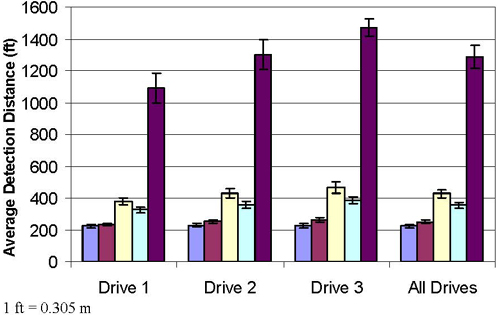
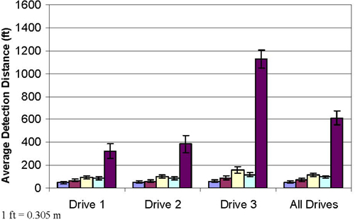
As is evident in the table, the sample of participants in this experiment performed extremely well in correctly detecting the direction of the curve ahead (99.7 percent correct overall). The participants were also quite confident in their judgments of curve direction, making 97.5 percent of their overall responses without any corrections. The sample of participants did not perform as well in correctly detecting the severity of the curve ahead (82.5 percent correct overall). Nevertheless, since guessing would yield 50 percent correct responding, even their performance on the severity detection task was well above chance. If the normal approximation to the binomial is employed to the worst case in table 6 (p = 0.787; P = 0.500; n = 432), the probability of obtaining a sample correct response rate of 78.7 percent when the population correct response rate is 50.0 percent is extremely small (z = 11.91, p < 0.001). Thus, although the participants were making a substantial number of errors in detecting the severity of the curve ahead, they were still performing considerably better than chance (over 80 percent correct). As might be expected, their confidence in these severity judgments was not as strong as their confidence in the corresponding direction judgments, making only 90.4 percent of their overall severity responses without any corrections as opposed to 97.5 percent of their overall direction responses. Still, over 90 percent of all severity judgments were made without the necessity to make a change. This reduced performance on curve severity judgments relative to curve direction judgments indicates that additional visual cues may need to be provided to the driver to assist in detecting the severity of approaching curves. Of the 379 errors made in estimating curve severity, 49.9 percent were made estimating right curves, and 50.1 percent were made estimating left curves. Thus, it was equally easy to estimate the direction of right or left curves. Of the same 379 errors, 42.7 percent were made estimating sharp curves, and 57.3 percent were made estimating gentle curves. If the normal approximation to the binomial is employed again, this discrepancy is extremely unlikely (z = 2.84, p < 0.003). The participants found it easier to estimate the severity of sharp curves than gentle curves. This outcome might be expected since both sharp and gentle curves had the same deflection angle of 60 degrees. This situation resulted in the sharper curves having a more compressed forward field of view, providing more simultaneous foveal visual cues for estimating the radius of curvature. It is interesting to note that the streaming PMDs condition performed the worst in terms of correct curve severity estimation. This result is surprising considering that the streaming PMDs condition was the only visual stimulus which incorporated a supplemental coding scheme to indicate curve severity. Apparently, this coding scheme was difficult to comprehend, and the rapid moving light patterns may have obscured other cues normally used to estimate curve severity (e.g., radius of curvature). Curve Direction Detection Distance Figure 18 shows the average curve direction detection distance for the five visibility treatments as a function of the number of the drive. The right side of the figure shows the results collapsed across all three drives. The error bars represent one standard error of the mean. Curve geometry had no effect on curve direction detection—both curve severity and direction effects were not statistically significant. However, both the treatment by drive (F (8, 28) = 3.13, p < 0.012) and the treatment by severity (F (4, 32) = 4.20, p < 0.008) interactions were statistically significant. The treatment by drive interaction is apparent in the positively accelerating shapes of the bar charts given in figure 18 when compared across drives. The treatment by severity interaction was reflected primarily in a skew for the streaming PMDs condition (not shown). Despite these interactions, a consistent pattern of average detection distance for curve direction across treatments is evident in figure 18 . This consistent pattern persists across all three drives and is also reflected across both curve severities (sharp versus gentle). Such a uniform pattern indicates the existence of a significant main effect of the visibility treatments themselves in addition to significant interactions with drive and curve severity. As evident in figure 18 , the five different visibility treatments were organized into three groups: pavement markings, conventional PMDs, and streaming PMDs. Over all drives, this main treatment effect was statistically significant (F (4, 32) = 66.9, p < 0.001). For curves with only pavement markings (baseline and edge lines), the direction of the curve could be detected from an average distance of 225 to 260 ft (68.6 to 79.2 m). By contrast, for curves with conventional reflectorized PMDs (single side PMDs and both sides PMDs), the direction of the curve could be detected at almost twice that distance between 385 and 465 ft (117 and 142 m). It is of interest to note that the both sides PMDs condition had a lower average direction detection distance (383 ft (117 m)) than the single side PMDs condition (466 ft (142 m)). This outcome may be the result of possible visual confusion caused by the larger number of PMD posts simultaneously in view for the both sides PMDs condition and their more complex geometric arrangement, making direction estimation more difficult. Nevertheless, as far as the speed reductions were concerned (see table 5 ), the both sides PMDs condition posed a more formidable visual array and slowed drivers down more than the single side PMDs condition by about 1 mi/h (1.6 km/h). The greatest improvement in direction detection distance was afforded by the LED-enhanced PMDs (streaming PMDs). For these sequential flashing PMDs, the average curve direction detection distance ranged from about 1,100 to 1,500 ft (335 m to 457 m), which was five times the baseline distance of about 225 to 260 ft (68.6 to 79.2 m). Since this streaming PMD condition was continuously operating and not activated by an approaching vehicle, the sequential pattern of flashing lights could be seen from a great distance. The four enhanced visibility treatment conditions represented a consistent order in terms of their effectiveness in increasing the distance at which the participants could detect the direction of curves ahead in the roadway. As can be seen in figure 18 , a similar order was maintained across all three drives, and this order was the same for all drives combined. Similar to what was done for vehicle speed, the relative detection distance advantages offered by the different treatments may be rounded to 5–ft (1.52–m) increments and taken as a figure of merit. When this is done, the following order was observed for direction detection distance from least effective to most effective: edge lines (25 ft (7.62 m)), both sides PMDs (130 ft (39.6 m)), single side PMDs (200 ft (61.0 m)), and streaming PMDs (1,065 ft (325 m)). For all three drives, the most dramatic improvement in average direction detection distance was associated with the streaming PMDs condition, a 1,065–ft (325 m) advantage over baseline in the combined case. Pair–wise ANOVA comparisons were made between the baseline condition and each additional visibility enhancement as well as between neighboring pairs in the above order of treatment effectiveness. These pair–wise comparisons were only conducted on the combined data from drives 1 and 2 since the instructions to the participants changed on day 3. All of these seven pair–wise comparisons revealed a statistically significant treatment effect. Thus, as concerns enhancing direction detection distance for curves, the four safety countermeasures can be ranked as indicated above. The enhanced direction detection distance for the streaming PMDs condition was increased to a 1,247–ft (380–m) advantage relative to the baseline when only drive 3 data were considered. The corresponding advantage relative to the baseline for drive 2 was 1,079 ft (329 m). Just prior to drive 3, the participants were informed of the meaning of the streaming PMD coded cues, including the cue for direction. This change in instructions could have been responsible for the observed increase in average detection distance for drive 3. Comparison of the advantages from drives 2 and 3 indicated that, in terms of direction detection distance, explaining the direction cue to the participants could result in a possible 16–percent advantage over having the participants figure out the meaning for themselves. However, this increased advantage is relatively small and could be due to learning which might have taken place even if no additional information had been provided in the instructions. Figure 18 also reveals a consistent adaptation or learning effect across the three drives, with the average curve direction detection distance increasing in each category with progressive drives. This drive effect was statistically significant (F (2, 34) = 20.2, p < 0.001). For the streaming PMDs condition, the drive 1 direction detection distance advantage was 864 ft (263 m) relative to the baseline, and the drive 2 advantage was 1,079 ft (329 m) for a gain of approximately 25 percent. If adaptation were linear, the detection distance advantage might be expected to be about 1,348 ft (411 m) for drive 3, which was greater than the 1,247 ft (380 m) that was observed. In fact, this 25–percent adaptation effect could completely account for the 16–percent increased advantage attributed earlier to being informed of the curve direction cue encoded in the streaming PMDs condition. Thus, the research participants were likely learning the meaning of the curve direction cue on their own. This cue was highly intuitive (streaming toward the right meant a right curve was approaching, and streaming toward the left meant a left curve was approaching) and probably did not require additional instructions for most of the research participants. The results of the questionnaire revealed a similar high degree of learning. After drive 2, before receiving any instructions, 83 percent of the participants knew the meaning of the direction cue. After drive 3 and receiving the instructions, 97 percent knew the meaning. Curve Severity Detection Distance Overall, similar relative results were found for the average distance at which the participants could detect the severity of a curve ahead in the roadway, but the absolute magnitudes were smaller. Figure 19 shows the average curve severity detection distance for the five visibility treatments as a function of the number of the drive. Similar to direction detection distance, the right–hand side of figure 19 shows the severity detection distance results collapsed across all three drives. Figure 18. Graph. Average curve direction detection distance as a function of drive.
Figure 19. Graph. Average curve severity detection distance as a function of drive. For severity detection distance, the effects of curve geometry were mixed. The sharp curves (222 ft (67.7 m)) had a greater average detection distance than the gentle curves (158 ft (48.2 m)). This curve severity effect was statistically significant (F (1, 35) = 40.6, p < 0.001), but the curve direction effect was not. In addition, there were two statistically significant interactions, the same two as were found for curve direction detection distance: (1) treatment by drive (F (8, 28) = 12.1, p < 0.001) and (2) treatment by severity (F (4, 32) = 5.48, p < 0.002). These interactions were reflected in the data relationships in the same way as for direction detection distance. There was also a statistically significant treatment by severity by direction interaction (F (4, 32) = 2.84, p < 0.004). A consistent pattern of average detection distance for curve severity across treatments is evident in figure 19 . This consistent pattern persists across all three drives, both curve severities and both curve directions. As evident in figure 19 , for severity detection distance, the five different visibility treatments organized themselves into two major groups: (1) streaming PMDs and (2) all others. For all conditions other than streaming PMDs, the average curve severity detection distance was about 55 to 115 ft (16.8 to 35.1 m). The average curve severity detection distance was much greater for the streaming PMDs condition (612 ft (187 m)). Across all drives, this treatment effect was statistically significant (F (4, 32) = 28.0, p < 0.001). Figure 19 also reveals a consistent adaptation or learning effect across the three drives, with the average curve severity detection distance increasing in each category with progressive drives similar to what was found for curve direction detection distance in figure 19 . This drive effect for severity detection distance was statistically significant (F (2, 34) = 42.5, p < 0.001). As with direction detection, the most dramatic improvement in average severity detection distance was associated with the streaming PMDs. For the streaming PMDs condition, on drives 1 and 2, the participants could detect curve severity at a distance of about 325 to 385 ft (99.1 to 117 m) with no special instructions as to the meaning of the curve severity cue. On drive 3, after the participants were informed of the meaning of the severity cue, the average curve severity detection distance increased to about 1,127 ft (344 m), representing an advantage of 1,074 ft (327 m) relative to the baseline condition. Since the corresponding day 2 advantage relative to the baseline was 333 ft (102 m), providing information to the participants concerning the severity cue coded in the streaming PMD lights resulted in a 300–percent increase in relative detection distance advantage over letting the participants figure out the meaning for themselves. The participants had difficulty learning the meaning of the curve severity cue on their own. In terms of severity detection distance, their performance improved dramatically after being informed of the meaning of the curve severity cue. Such an increase is not likely to be the result of adaptation, as can be seen in figure 19 . For the streaming PMDs condition, the detection distance advantage in the first drive was 271 ft (82.6 m) relative to the baseline, and the advantage for the second drive was 333 ft (102 m) for a gain of only about 23 percent. If adaptation was linear, the detection distance advantage might be expected to be about 410 ft (125 m) for drive 3 instead of the 1,074 ft (327 m) that was observed. The results of the questionnaire revealed a similar picture. After drive 2 before receiving any instructions, only 64 percent of the participants knew the meaning of the severity cue. After receiving the instructions for drive 3, 97 percent of the participants knew the meaning. Except for the streaming PMDs condition, the average curve severity detection distances in figure 19 were much shorter than the corresponding average curve direction detection distances in figure 18 by a factor of two to four times. This outcome indicates that at a given distance ahead of a curve, other factors being equal, detecting the direction (right versus left) of the curve is likely to be easier than detecting the severity (radius) of the curve. To make performance equivalent for the two curve features, additional visual information would need to be provided to the driver in the form of distinct cues for curve severity. Relative to the baseline, the four enhanced visibility treatment conditions represented a consistent order in terms of their effectiveness in increasing the distance at which the participants could detect the severity of curves ahead in the roadway. This relationship was discernable despite the fact that, except for the streaming PMDs condition, all of the average detection distance values were rather low and close together. As can be seen in figure 19 and table 7 (columns 4 and 5), a similar order was maintained across all three drives, and this order was the same for all drives combined. If increased curve severity detection distance is taken as the figure of merit, this order was as follows (from least effective to most effective): edge lines (20 ft (6.1 m)), both sides PMDs (45 ft (13.7 m)), single side PMDs (65 ft (19.8 m)), and streaming PMDs (560 ft (170 m)). Pair–wise ANOVA comparisons were conducted as was done for direction detection distance. All of these seven pair–wise comparisons revealed a statistically significant treatment effect except for two. The first exception was between the baseline and the edge lines. In this experiment, there was no advantage of adding edge lines for increasing severity detection distance. The second exception was between single side PMDs and both sides PMDs. In this case, both of these conditions were statistically different from the baseline. However, for detecting the severity of curves ahead, it did not matter whether reflectorized PMDs were on one side of the curve or on both sides. Thus, for detecting the severity of curves, the safety countermeasures devolved into only two ranks: both reflectorized PMDs (45 to 65 ft(13.7 to 19.8 m)) and streaming PMDs (560 ft (171 m)). For all drives, table 7 shows the average feature detection distance and distance advantage for the different curve visibility treatment conditions. Columns 2 and 4 give the data for the right–hand portions of figure 18 and figure 19 . For each treatment condition, columns 3 and 5 give the relative advantages of the different treatments in increasing feature detection distance relative to the baseline. The visibility treatments in table 7 are arranged in order of increasing effectiveness in achieving a greater feature detection distance for both curve direction and curve severity. The last row in the table is an exception. This row shows the average feature detection distance for drive 3 only when the participants had just been informed of the meaning of the direction and severity cues coded in the patterns of steaming PMDs. An examination of the standard errors in table 7 reveals that most were below 25 ft (7.6 m) except for the streaming PMDs condition. For most treatments, when comparing pairs of distances in the table, distance reductions of 50 ft (15.2 m) or greater were likely to be statistically significant. In the case of streaming PMDs, this distance reduction criterion increased to150 ft (45.7 m) or greater due to increased variability in the detection distance data for this condition. Table 7. Average feature detection distance and distance advantage for curves.
1 ft = 0.305 mNote: Standard error (SE) is shown in parentheses. TownsSpeed Profiles for TownsFigure 20 shows the average vehicle speed as a function of distance from the beginning of the town for the six different town treatment conditions. Figure 21 refers to corresponding acceleration data which will be described later. The data represent speed profiles in terms of averages across all participants and all days. The error bars represent one standard error of the mean. Data are shown for all 10 measurement locations. Positive distances indicate measurement locations ahead of the town, and negative distances indicate locations in the town. However, since speed calming inside the town was the major focus, all statistical tests were conducted on the five locations in the town from the beginning of the town (zero ft (zero m)) to the end of the town (–450 ft (–137 m)). As with the curve data, the town data were also analyzed according to a MANOVA approach to repeated measures. Figure 20. Graph. Average speed as a function of the distance from the beginning of the town. Figure 21. Graph. Average acceleration as a function of the distance from the beginning of the town. The speed profiles in figure 20 indicate a gentle deceleration followed by a plateau. As indicated by this distinct overall shape, the location effect was statistically significant (F (4, 31) = 11.1, p < 0.001). The drivers slowed down from 50 mi/h (80.5 km/h) at 1,000 ft (305 m) before the town to 32–38 mi/h (51.5–61.2 km/h) at the middle of the town depending on the type of treatment. The treatments were organized into three groups: (1) baseline and bulb-outs (baseline, curb and gutter bulb-outs, and painted bulb-outs), (2) parked cars, and (3) chicanes (curb and gutter chicanes and painted chicanes). This treatment effect was statistically significant (F (5, 30) = 12.5, p < 0.001). However, the shapes of the speed profiles were different for the various traffic-calming treatments, in particular for the chicanes and parked cars conditions. As might be expected from the different shapes of the functions portrayed in figure 20 , there was a statistically significant location by treatment interaction (F (20, 15) = 3.05, p < 0.016). The effect of drive was not statistically significant; thus, for speed in the town, there was no apparent adaptation or learning effect over the three drives. The bulb-outs were the least effective traffic-calming countermeasures, slowing drivers down by only 1 to 1.5 mi/h (1.6 to 2.4 km/h) through the town relative to the baseline. The parked cars condition was intermediate in its effectiveness, slowing drivers down by 4 to 5 mi/h (6.4 to 8 km/h) relative to the baseline at the middle of the town. The chicanes were the most effective in slowing the drivers down through the town as a whole, slowing them by 6 to 9 mi/h (9.7 to 14.5 km/h) through the town relative to the baseline. The curb and gutter chicanes were more effective than the painted chicanes by about 1 to 3 mi/h (1.6 to 4.8 km/h), and all of these differences were statistically significant (see below). The shapes of the speed profile functions were similar for all of the five types of safety countermeasures except the chicanes. For all other countermeasures, the minimum speed was achieved near the middle of the town or slightly further into the town. For the chicanes, the minimum speed was achieved at the beginning and end of the town where the chicanes were located. In the town itself, the speed increased for the chicane conditions, reaching a local maximum at the middle of the town and decreasing again for the second chicane. Across all five locations within the town, pair-wise ANOVA comparisons were made between the baseline condition and each individual speed–calming enhancement as well as between neighboring pairs in order of treatment effectiveness. All of the nine pair–wise comparisons revealed a statistically significant treatment effect except for the comparison between curb and gutter bulb–outs and painted bulb–outs. Both bulb–out conditions performed better than the baseline, but there was no statistically significant difference between the two implementations. This experiment found that the cheaper painted bulb–outs were just as effective as the more expensive curb and gutter bulb–outs, but neither one produced a substantial speed reduction effect (only about 1 mi/h (1.6 km/h)). Speed Reductions for TownsThe beginning and middle of the town were important locations for measuring driver behavior. These locations bound the first part of the town where it was important that the driver slowed the vehicle down to a safe speed for entering and driving through the town. Table 8 shows the average speed at the beginning and at the middle of the town along with the corresponding speed reduction advantages relative to the baseline speed. If the relative speed reduction advantage at the beginning of the town was taken as the figure of merit (rounded to 0.5 mi/h (0.8 km/h)), the following order was observed from least effective to most effective: both bulb–outs (about 1 mi/h (1.6 km/h)), parked cars (4 mi/h (6.4 km/h)), painted chicanes (6 mi/h (9.7 km/h)), and curb and gutter chicanes (9 mi/h (14.5 km/h)). If the figure of merit was shifted to the middle of the town, the rankings have a slightly different order: both bulb–outs (about 1 mi/h (1.6 km/h)), painted chicanes (4 mi/h (6.4 km/h)), parked cars (4.5 mi/h (7.2 km/h)), and curb and gutter chicanes (5 mi/h (8 km/h)). As a result of the treatment by location interaction observed above, in this case, parked cars and painted chicanes changed places in the rank order. At the middle of town location, the speeding up in the center of the town that was observed with the chicanes offset some of the apparent advantage of the chicane treatment. This increase in speed was as much as 1 to 3 mi/h (1.6 to 4.8 km/h) faster than in the chicane itself. Table 8. Average speed and speed reduction advantage in towns (mi/h).
1 mi = 1.61 kmNote: Standard error (SE) is shown in parentheses. Since the effects of the various treatments were different for the beginning and middle of the town, both locations need to be considered in comparing the effectiveness of the various speed-calming treatments investigated in the current experiment. Therefore, pair–wise statistical comparisons were computed for the 30 combinations of all 6 average speeds both at the beginning of the town (column 2) and at the middle of the town (column 4). For the beginning of the town, all 30 pair–wise comparisons revealed statistically significant differences except the following three cases: (1) baseline versus painted bulb–outs, (2) baseline versus curb and gutter bulb–outs, and (3) painted bulb–outs versus curb and gutter bulb–outs. At the beginning of the town, the two types of bulb–outs were not different from each other, and neither type was different from the baseline. At this location, the only treatments which resulted in a speed reduction were the parked cars and chicanes conditions. For the middle of the town, all 30 pair–wise comparisons revealed a statistically significant difference except the following three cases: (1) painted bulb–outs versus curb and gutter bulb–outs, (2) parked cars versus painted chicanes, and (3) parked cars versus curb and gutter chicanes. At the middle of the town, the two types of bulb–outs were not different from each other, but both types were different from the baseline. In addition, there was no difference in speed reduction between the parked cars and either type of chicane implementation. At this location, the only treatments which resulted in a substantial speed reduction were the parked cars and chicanes conditions. Both types of bulb–outs had a very small effect on speed reduction (about 1 mi/h (1.6 km/h)). Both chicane conditions were characterized by an increase in average vehicle speed in the middle portion of the town. This was to be expected since the chicanes themselves were located at both ends of the town. Under the chicane conditions, no speed–calming measures were employed in the middle portion of the town, allowing the drivers to speed up in the middle portion of the town only to slow down again for the second chicane at the exit from the town. Overall, parked cars and chicanes were considerably more effective than bulb–outs in slowing driver speed. In addition, the parked cars condition was associated with a more steady decrease in speed beginning further away from the town when compared with any of the other treatments. For example, at 100 ft (30.5 m) from the town, the parked cars condition had an average vehicle speed of 3 mi/h (4.8 km/h) less than the baseline condition. Such an outcome might be expected since the parked cars tended to be visible from further away than any of the other speed–calming treatments. The speed profiles for the towns also revealed that the participants were already slowing down from the instructed speed of 55 mi/h (88.5 km/h) in the tangents to about 51 mi/h (82 km/h) at 1,000 ft (305 m) before the town. This was also to be expected since the towns were driven in daylight conditions and could be seen by the driver from a greater distance (more than 1,000 ft (305 m)). Acceleration Profiles for TownsFigure 21 shows the average longitudinal acceleration of the vehicle as a function of distance from the beginning of the town for the six different speed–calming treatment conditions. As was the case for curves, the data represent acceleration profiles which complement the corresponding speed profiles portrayed in figure 20 . As a result of the computation method, the data are shown for nine intermediate distance values (locations). As was the case for the speed profiles for the towns, all statistical tests were conducted only on the five locations inside the town. The acceleration profiles for the towns had a gentle overall U–shape. As expected from this overall shape, the location effect was statistically significant (F (3, 30) = 21.6, p < 0.001). The major exception is that the chicanes had a pronounced jagged, saw–tooth shape in the middle. This saw–tooth pattern represents rapid deceleration to navigate the first chicane at the beginning of the town, acceleration through the first part of the town, and somewhat less rapid deceleration to navigate the second chicane toward the end of the town. In general, the acceleration profiles for the towns were organized into two groups of treatments: the chicanes and all other treatments with one exception for the parked cars condition. The parked cars condition revealed somewhat lower deceleration values before the town. Thus, within the town, decidedly different shapes were observed for the acceleration profiles for the six different traffic–calming treatments. As would be expected from these differently shaped profiles, the treatment by location interaction was statistically significant (F (15, 18) = 4.77, p < 0.001). However, as concerns the town acceleration profiles as a whole, the treatment effect was not statistically significant (F (5, 28) = 2.47, p < 0.056). In this case, the interaction between treatment and location was the significant factor. Different traffic–calming treatments produced different acceleration profiles. |