Prediction of the Expected Safety Performance of Rural Two-Lane Highways
6. IMPLEMENTATION OF THE ACCIDENT PREDICTION ALGORITHM WITHIN THE IHSDM
The accident prediction algorithm is intended to help the user to make unbiased estimates of the expected safety performance for any given geometric design alternative for a specific highway improvement project. Complete evaluation of one or more proposed geometric design alternatives for a particular project will require the user to determine, for comparative purposes, both the safety performance of the current design and the expected future safety performance of that current design if nothing is done to change the roadway (the “do nothing” or “baseline” alternative).
This section of the report describes the implementation of the accident prediction algorithm within the IHSDM. Procedures are presented by which the algorithm can be used to make unbiased estimates of the:
- Expected safety performance of one or more geometric design alternatives for a planned roadway that has not yet been constructed.
- Recent or current safety performance of an existing roadway considering both the predicted safety performance of the roadway and its observed accident history.
- Expected safety performance of the existing roadway in the future if the geometrics are left unchanged (the ADT may change, of course).
- Expected safety performance of one or more proposed geometric design alternatives for improving the existing roadway.
This section describes two methods for producing these estimates—one without and one with consideration of site-specific accident history data for the project of interest. The first procedure described is used when no site-specific accident history data are available. This first procedure is applicable to planned roadways that have not yet been constructed and to existing roadways where, for whatever reason, site-specific accident history data are not available to the analyst. The second procedure described is used when site-specific accident history are available. This procedure incorporates an Empirical Bayes (EB) approach to combining estimates from the accident prediction algorithm and site-specific accident history data. Examples of the EB procedure are presented later in this section.
Site-specific accident history data make an important contribution to increasing the accuracy of predictions of the expected safety performance of highway facilities. Therefore, the analyst should seek to obtain and use site-specific accident history data and apply the EB procedure whenever possible.
The procedures presented here can be applied to any existing two-lane highway or to any two-lane highway improvement project that retains the basic two-lane character of the facility. Two-lane highway improvements evaluated with these procedures can include addition of a third or fourth lane over a short distance to improve passing opportunities on the highway. Thus, the procedures can evaluate passing lanes that create a three-lane cross section and short four-lane sections that are operationally equivalent to side-by-side passing lanes. Such added lanes do not normally exceed 3.2 km (2 mi) in length. The procedures do not address widening of a two-lane highway to a four-lane cross section for an extended length. It is hoped that appropriate procedures for four-lane highways will be developed in the future so that analysis of two-lane to four-lane widening projects will be possible within the IHSDM.
Accident Prediction When Site-Specific Accident History Data are not Available
The accident prediction algorithm is intended to estimate the expected accident frequency for any specified geometric design alternative and for any specified evaluation period. The specified geometric design alternative to which the algorithm is applied can be either the existing roadway (i.e., the “do-nothing” alternative), a proposed geometric design improvement to the existing roadway, or a proposed roadway that has not yet been constructed. This first procedure is applicable only to a project for which no site-specific accident history data are available. The algorithm can be used to compare the expected safety performance of several geometric alternatives by applying the algorithm separately to each alternative for the same evaluation period and comparing the results. When no site-specific accident history data are available, the duration of the evaluation period may be one year or any multiple of one year. The accident prediction algorithm is applied in IHSDM to any specific geometric design alternative in a series of straight forward steps, as follows:
- Step 1—Define the limits of the project and determine the geometrics of the project for which the expected safety performance is to be predicted.
- Step 2—Divide the project into individual homogeneous roadway segments and intersections.
- Step 3—Determine the geometric design and traffic control features for each individual roadway segment and intersection.
- Step 4—Determine the ADTs for each roadway segment and intersection during each year for which the expected safety performance is to be predicted.
- Step 5—Select an individual roadway segment or intersection for evaluation. If there are no more roadway segments or intersections to be evaluated, go to step 13.
- Step 6—Select a particular year of the specified evaluation period for the roadway segment or intersection of interest. If there are no more years to be evaluated for that roadway segment or intersection, go to step 12.
- Step 7—Apply the appropriate base model to determine the predicted accident frequency for nominal or base conditions for the selected year.
- Step 8—Multiply the result obtained in step 7 by the appropriate calibration factor for a specific State or geographical region.
- Step 9—Multiply the result obtained in step 8 by the appropriate AMFs representing safety differences between the nominal or base conditions and the actual geometrics and traffic control of the roadway segment or intersection.
- Step 10—Estimate the expected distribution accident severities and accident types for the roadway segment or intersection from the default distributions of accident severity and accident type.
- Step 11—If there is another year to be evaluated for the selected roadway segment or intersection, return to step 6. Otherwise, proceed to step 12.
- Step 12—If there is another roadway segment or intersection to be evaluated, return to step 5. Otherwise, proceed to step 13.
- Step 13—Summarize and present the predictions in useful formats for the IHSDM user.
Figure 5 presents a flow diagram of the accident prediction algorithm incorporating these steps. Each of these steps is described below:
Step 1—Define the limits of the project and determine the geometrics of the project for which the expected safety performance is to be predicted.
The project evaluated can represent either an existing roadway or a design alternative for a proposed improvement project. The geometric design features of the project and the traffic control at each intersection must be documented. The geometric design features are determined from either a plan of the existing roadway available in the CAD system or from data entered by the user. If CAD data are to be used, a program must be developed to interrogate the CAD file, determine the geometrics of the project, and store those geometric data in a format that can be used by IHSDM.
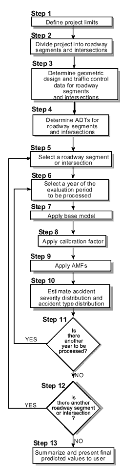
Figure 5. Flow Diagram of the Accident Prediction Algorithm When No Site-Specific History Data Are Available.
Step 2—Divide the project into individual homogeneous roadway segments and intersections.
The next step is to divide the project into individual homogeneous roadway segments and intersections. The roadway must be divided into homogeneous segments. A new homogeneous segment begins at each intersection where the value of one of the following variables changes:
- Average daily traffic volume (veh/day).
- Lane width.
- Shoulder width.
- Shoulder type.
- Driveway density (driveways per mile).
- Roadside hazard rating.
Also, a new analysis section starts at any of the following locations:
- Intersection.
- Beginning or end of a horizontal curve.
- Point of vertical intersection (PVI) for a crest vertical curve, a sag vertical curve, or an angle point at which two different roadway grades meet.
- Beginning or end of a passing lane or short four-lane section provided for the purpose of increasing passing opportunities.
- Beginning or end of a center two-way left-turn lane.
Step 3—Determine the geometric design and traffic control features for each individual roadway segment and intersection.
For each roadway segment, the following geometric and traffic control features must be quantified:
- Length of segment (mi).
- ADT (veh/day).
- Lane width (ft).
- Shoulder width (ft).
- Shoulder type (paved/gravel/composite/turf).
- Presence or absence of horizontal curve (curve/tangent).
- Length of horizontal curve (mi), if the segment is located on a curve. [This represents the total length of the horizontal curve, even if the curve extends beyond the limits of the roadway segment being analyzed.]
- Radius of horizontal curve (ft), if the segment is located on a curve.
- Presence or absence of spiral transition curve, if the segment is located on a curve. [This represents the presence or absence of a spiral transition curve at the beginning and end of the horizontal curve, even if the beginning and/or end of the horizontal curve are beyond the limits of the segment being analyzed.]
- Superelevation of horizontal curve, if the segment is located on a horizontal curve.
- Grade (percent), considering each grade as a straight grade from PVI to PVI (i.e., ignoring the presence of vertical curves).
- Driveway density (driveways per mi).
- Presence or absence of a passing lane to increase passing opportunities.
- Presence or absence of a short four-lane Section to increase passing opportunities.
- Presence or absence of a two-way left-turn lane.
- Roadside hazard rating.
For each intersection, the following geometric and traffic control features must be quantified:
- Number of intersection legs (3 or 4).
- Type of traffic control (minor-road STOP, all-way STOP, minor-road YIELD control, or signal).
- Intersection skew angle (degrees departure from 90 degrees, with a + or - sign indicating the direction of the departure).
- Number of major-road approaches with intersection left-turn lanes (0, 1, or 2).
- Number of major-road approaches with intersection right-turn lanes (0, 1, or 2).
- Number of intersection quadrants with deficient intersection sight distance (0, 1, 2, 3, or 4).
The values of these geometric and traffic control parameters for roadway segments and intersections will be determined from the CAD system, from existing data files, or from data supplied by the user.
Step 4—Determine the ADTs for each roadway segment and intersection during each year for which the expected safety performance is to be predicted.
For each roadway segment and for the major- and minor-road approaches to each intersection, ADT data are needed for each year of the period to be evaluated. Ideally, these ADT data will already be available in a file or they will be entered by the user. If ADTs are available for every roadway segment, the major-road ADTs for intersection approaches can be determined without additional data being supplied by the user. If the ADTs on the two major-road legs of an intersection differ, the average of the two ADT values should be used for the intersection. For a three-leg intersection, the user should enter the ADT of the minor-road leg. For a four-leg intersection, the user should enter the average of the ADTs for the two minor-road legs.
In many cases, it is expected that ADT data will not be available for all years of the evaluation period. In that case, the analyst should interpolate or extrapolate as appropriate to obtain an estimate of ADT for each year of the evaluation period. If the analyst does not do this, the following default rules are applied within the accident prediction algorithm to estimate the ADTs for years for which the data are not available. If ADT data are available for only a single year, that same value is assumed to apply to all years of the before period. If two or more years of ADT data are available, the ADTs for intervening years are computed by interpolation. ADTs for years before the first year for which data are available are assumed to be equal to the ADT for that first year; ADTs for years after the last year for which data are available are assumed to be equal to the last year (i.e., no extrapolation is used by the algorithm).
Step 5—Select an individual roadway segment or intersection for evaluation. If there are no more roadway segments or intersections to be evaluated, go to step 13.
Roadway segments and intersections are evaluated one at a time. Steps 6 through 11, described below, are repeated for each roadway segment and intersection.
Step 6—Select a particular year of the specified evaluation period for the roadway segment or intersection of interest. If there are no more years to be evaluated for that roadway segment or intersection, go to step 12.
The individual years of the evaluation period are evaluated one year at a time for any particular roadway segment or intersection. Separate estimates are made for each year because several of the AMFs considered in step 9 are dependent on the ADT of the roadway segment or intersection, which may change from year to year. Steps 7 through 10, described below, are repeated for each year of the evaluation period as part of the evaluation of any particular roadway segment or intersection.
Step 7—Apply the appropriate base model to determine the predicted accident frequency for nominal or base conditions for the selected year.
The predicted accident frequency for nominal or base conditions is determined with one of the following base models:
| •Roadway segments |
Equation (6). |
| •Three-leg STOP-controlled intersections |
Equation (8). |
| •Four-leg STOP-controlled intersections |
Equation (10). |
| •Four-leg signalized intersections |
Equation (12). |
The ADT(s) used in the base model should be the ADT(s) for the selected year of the evaluation period.
Step 8—Multiply the result obtained in step 7 by the appropriate calibration factor.
The calibration factors used in step 8 are the calibration factor for roadway segments (Cr) and the calibration factor for intersections (Ci) discussed in section 3 and appendix C of this report.
Step 9—Multiply the result obtained in step 8 by the appropriate AMFs representing safety differences between the nominal or base conditions and the actual geometrics and traffic control of the roadway segment or intersection.
The AMFs for roadway segments and intersections are those described in Section 4 of this report. Steps 8 and 9 together implement equations (13) and (14).
Step 10—Estimate the expected distribution of accident severities and accident types for the roadway segment or intersection of interest from the default distributions of accident severity and accident type.
The predictions of accident frequencies are supplemented by breaking down those frequencies by accident severity and by accident type. This can provide the IHSDM user with greater insight about safety conditions within the project. The accident severity and accident type estimates are based on the default distributions of accident severity and accident type presented in Tables 1 and 2, respectively. These default distributions may be changed by IHSDM users as part of the calibration process.
Step 11—If there is another year to be evaluated for the selected roadway segment or intersection, return to step 6. Otherwise, proceed to step 12.
This step creates a loop through steps 7 to 10 that is repeated for each year of the evaluation period for each of the individual roadway segments and intersections within the project.
Step 12—If there is another roadway segment or intersection to be evaluated, return to step 5. Otherwise, proceed to step 13.
This step creates a loop through Steps 6 to 11 that is repeated for each roadway segment and intersection within the project.
Step 13—Summarize and present the predictions in useful formats for the IHSDM user.
In the final step, the predicted accident frequencies are summarized and presented in useful formats for IHSDM users. The data presented include, at a minimum:
- Accident frequencies for the project as a whole including:
-
-- Total accident frequency.
-- Accident frequency by severity level.
-- Accident frequency by accident type.
- Accident frequencies for individual roadway segments and intersections, expressed as accident rates per mi per year or accident rate per million veh-mi for roadway segments and accident rates per million entering vehicles for intersections, so that accident “hot spots” that might be corrected through design improvements are evident.
Estimated accident frequencies could also be broken down by individual years of the evaluation period. However, this is not normally done because the combined estimates across all years of the evaluation period are generally of greatest interest to safety analysts. Predicted accident frequencies for a multiyear period are likely to be more accurate than predicted accident frequencies for any particular year.
Accident Prediction When Site-Specific Accident History Data are Available
Consideration of site-specific accident history data in the accident prediction algorithm increases the accuracy of the predicted accident frequencies. When at least 2 years of site-specific accident history data are available for the project being evaluated, and when the project meets certain criteria discussed below, the accident history data should be used. When considering site-specific accident history data, the algorithm must consider both the existing geometric design and traffic control for the project (i.e., the conditions that existed during the before period while the accident history was accumulated) and the proposed geometric design and traffic control for the project (i.e., the conditions that will exist during the after period, the future period for which accident predictions are being made). The EB procedure discussed below provides a method to combine predictions from the algorithm with site-specific accident history data.
Situations in Which the EB Procedure Should and Should Not Be Applied
The applicability of the EB procedure depends on the availability of observed accident history data and the type of improvement project being evaluated. If no observed accident history data are available, application of the EB procedure is infeasible and should not be considered. If observed accident history data are available, the applicability of the EB procedure depends on the type of improvement project being evaluated.
The EB procedure should be applied for the following improvement types whenever observed accident history data are available:
- Sites at which the roadway geometrics and traffic control are not being changed (e.g., the “do-nothing” alternative).
- Projects in which the roadway cross Section is modified but the basic number of lanes remains the same. This would include, for example, projects for which lanes or shoulders were widened or the roadside was improved, but the roadway remained a rural two-lane highway.
- Projects in which minor changes in alignment are made, such as flattening individual horizontal curves while leaving most of the alignment intact.
- Projects in which a passing lane or a short four-lane section is added to a rural two-lane highway to increase passing opportunities.
- Any combination of the above improvements.
The EB procedure is not applicable to the following types of improvements:
- Projects in which a new alignment is developed for at least 50 percent of the project length. In this case, the procedure used when no site-specific accident history data are available, as described above, should be applied because there is no reason why the accident history of the old alignment should be used as a predictor of future accident frequency on the new alignment. In others words, there is no reason to think that the new roadway will have substantially higher (or lower), accident experience, simply because the existing roadway has high (or low) accident experience. For cases in which the user is concerned that a particular geographic area or corridor has higher or lower accident experience than expected, a special study may be performed to revise the calibration factor accordingly.
- Individual intersections at which the basic number of intersection legs or type of traffic control is changed as part of a project. The EB procedure can be applied to the rest of any project containing such an intersection, but the intersection itself should be omitted.
The reason that the EB procedure is not used for these project types is that the observed accident data for a past time period is not necessarily indicative of the accident experience that is likely to occur in the future, after such a major geometric improvement. When the EB procedure does not apply, the accident prediction algorithm without the EB procedure (described earlier in this section of the report) is used to determine the expected safety performance for a project during some future time period. When the EB procedure does apply, the accident prediction algorithm, including the EB procedure, is applied as described below.
Empirical Bayes Procedure
The EB procedure provides a methodology to combine the accident frequencies predicted by the accident prediction algorithm (Np) with the accident frequency from the site-specific accident history data (O). The EB procedure uses a weighted average of Np and O. This procedure constitutes Step 9 of the step-by-step methodology presented below. A previous application of the EB methodology in before-and-after safety evaluations of intersections converted from STOP to signalized control is presented by Griffith.(40)
The expected accident frequency considering both the predicted and observed accident frequencies is computed as:
| Ep = w (Np) + (1-w) O |
(32)
|
where:
| Ep |
= |
expected accident frequency based on a weighted average of Np and No; |
| Np |
= |
number of accidents predicted by the accident prediction algorithm during a specified period of time (equal to Nrs for a roadway segment or Nint for an intersection); |
| w |
= |
weight to be placed on the accident frequency predicted by the accident prediction algorithm; and |
| O |
= |
number of accidents observed during a specified period of time. |
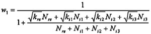
The weight placed on the predicted accident frequency is determined in the EB procedure as:
where:
| k |
= |
overdispersion parameter of the relevant base model of the accident prediction algorithm. |
The formulation of Equation (33) shows an inverse relationship between the magnitude of the accident frequency predicted by the algorithm, Np and the weight, w. Therefore, as the value of Np predicted by the algorithm increases, the weight placed on Np decreases. This relationship implies that the higher the expected accident frequency predicted by the algorithm for a particular location, the more the reliance that should be placed on the observed site-specific accident history and the less the reliance that should be placed on the model prediction itself. By contrast, when the model prediction is smaller, less reliance should be placed on the observed site-specific accident history and greater reliance should be placed on the model prediction.*
Table 23 shows the values of the overdispersion parameters (k) for the four base models used in the accident prediction algorithm.
The EB procedure works best if the roadway segments and intersections to which it is applied contain at least a specified minimum number of predicted accidents. The minimum accident frequency needed for application of the EB procedure is generally 1/k, where k is the overdispersion parameter of the relevant base model. In the accident prediction algorithm, this 1/k criterion is normally applied to the accident frequency for fatal and injury accidents because the frequency of fatal and injury accidents is usually less than the frequency of property-damage-only accidents and is always less than or equal to the total accident frequency. Where the fatal and injury accident frequency of particular roadway segments or intersections is less than 1/k, such segments and intersections may be aggregated into larger analysis units for application of the EB procedure.
In the accident prediction algorithm, the EB procedure is applied separately to the total predicted and observed accident frequencies and to the predicted and observed frequencies for two accident severity levels: fatal and injury accidents and property-damage-only accidents. Because the EB procedure is applied separately, the predicted fatal and injury accident and property-damage-only accident frequencies may not sum to the predicted total accident frequencies. A proportional adjustment to the predicted accident frequencies for the individual severity levels is made to correct this discrepancy.
* Equation (33) follows from the theoretical development of the EB approach by Hauer.(2) Hauer defines the weight in the EB procedure as (1+Var{k}/E{k})-1, where E{k} is the expected mean accident frequency and Var{k} is the variance of accident frequency. The expected mean accident frequency is best estimated by the model prediction, Np. Negative binomial regression modeling is based on the assumption that Var{k}=k(E{k})2. Therefore, it follows that the ratio Var{k}/E{k} can be estimated by k/Np, which leads to Equation (33).
Table 23. Overdispersion Parameters for Base Models and Minimum Accident Frequencies EB Procedure.
| Geometric element |
Overdispersion Parameter for base model (k) |
Minimum accident frequency for EB procedurea(1/k) |
| Roadway segment |
0.31 |
3 |
| Three-leg STOP-controlled intersection |
0.54 |
2 |
| Four-leg STOP-controlled intersection |
0.24 |
4 |
| Four-leg signalized intersection |
0.11 |
9 |
a Rounded for application in the EB procedure. Normally, this minimum accident frequency criterion is applied in the EB procedure to the predicted fatal and injury accident frequency.
If an EB analysis unit combines roadway segments and intersections, or more than one type of intersection, two additional factors must be accounted for. First, the overdispersion parameter, k, in the denominator of equation (33) is no longer uniquely defined, because two or more base models with differing overdispersion parameters must be considered. Second, it can no longer be assumed, as is normally done, that the expected numbers of accidents for the roadway segments and intersections, or for the different types of intersections, are statistically correlated with one another. Rather, an estimate of expected accidents should be computed based on the assumption that the different entities arestatistically independent (r=0) and on the alternative assumption that they are perfectly correlated (r=1). The expected accident frequency is then estimated as the average of the estimates for r=0 and r=1. The following equations implement this approach:
| w0 = |
1
|
(34)
|
|
|
1 +
|
krsNrs2 + ki1Ni12 +ki2Ni22 + ki3Ni32
|
|
|
Nrs + Ni1 + Ni2 + Ni3
|
|
E0 = w0 (Nrs + Ni1 + Ni2 + Ni3 ) + (1-w0)(Ors + Oi1 + Oi2 + Oi3)
|
(35)
|
|
|
(36)
|
|
E1 = w1 (Nrs + Ni1 + Ni2 + Ni3) + (1-w1)(Ors + Oi1 + Oi2 + Oi3)
|
(37)
|
where:
| w0 |
= |
weight placed on predicted accident frequency when accident frequencies for different roadway elements are statistically independent (r=0); |
| w1 |
= |
weight placed on predicted accident frequency when accident frequencies for different roadway elements are perfectly correlated (r=1); |
| E0 |
= |
expected accident frequency based on the assumption that different roadway elements are statistically independent (r=0); |
| E1 |
= |
expected accident frequency based on the assumption that different roadway elements are perfectly correlated (r=1); |
| Eau |
= |
expected accident frequency for an analysis unit made up of two or more roadway segments or intersections; |
| krs |
= |
overdispersion parameter for roadway segments (analogously, a subscript of i1 represents three-leg STOP-controlled intersections, i2 represents four-leg STOP-controlled intersections, and i3 represents four-leg signalized intersections); |
| Nrs |
= |
predicted total number of accidents for all roadway segments within the EB analysis unit (analogous for subscripts i1, i2, and i3); |
| Ors |
= |
observed total number of accidents for all roadway segments within the EB analysis unit (analogous for subscripts i1, i2, and i3). |
Example Application of the EB Procedure
The following discussion presents a numerical example to illustrate the application of the EB procedure. The example shows the application of the EB procedure to combine predicted accident frequencies for the period from 1989 through 1997 for roadway segments and intersections within a project site with the observed site-specific accident history for that same time period. The combined estimates of accident frequency resulting from application of the EB procedure represent an unbiased estimate of safety conditions during the period prior to construction of a proposed project at this site (the “before period”) and can subsequently be used in estimating the effect on safety of proposed alternative geometric design improvements to this site (the “after” period). The example illustrates the EB procedure, but does not illustrate the entire accident prediction methodology that incorporates the EB procedure; that methodology is presented later in this section of the report.
The example addresses two hypothetical roadway segments and one hypothetical intersection. Roadway segment 1 is a two-lane highway segment 1.6 km (1 mi) in length with an initial ADT of 2,000 veh/day. Over the 9-year period (1989-1997), the ADT varies up and down reaching 2,200 veh/day in 1997. Roadway segment 2 is a longer 8-km (5-mi) two-lane highway segment with a lower, but faster growing, ADT than segment 1. Intersection 1 is a four-leg STOP-controlled intersection located on segment 1. The intersection has a minor-road volume that increases from 500 veh/day in 1989 to 600 veh/day in 1997.
The first portion of the example shows the application of the EB procedure to roadway segment 1. This roadway segment was predicted to experience 4.2 accidents during the 9-year period (1989-1997), but actually experienced 6 accidents. Table 24 shows the application of the EB procedure which determines that the expected accident frequency for the roadway segment, considering both the predicted and observed values, is 5.2 accidents. Of these, it is expected that 3.3 would be fatal and injury accidents and 1.9 would be property-damage-only accidents.
While the computations in table 24 follow the EB procedure, the table shows that the predicted fatal and injury accident frequency for roadway segment 1 before application of the EB procedure was 1.4 accidents during the 9-year period. This does not meet the minimum accident frequency criterion (l/k) of three fatal and injury accidents for roadway segments shown in table 23. Thus, rather than relying on the results shown in table 24, it would be better to combine roadway segment 1 with another roadway segment before applying the EB procedure.
Table 25 presents the application of the EB procedure to roadway segment 2 in a manner analogous to table 24. Roadway segment 2 was predicted to experience 10.3 accidents during the 9-year period, but actually experienced 14 accidents. The table shows that the expected accident frequency for roadway segment 2, considering both the predicted and observed values, is 13.1 accidents during the 9-year period.
Roadway segment 2 was originally predicted to experience 3.3 fatal and injury accidents per year, so the minimum accident criterion for application of the EB procedure shown in table 23 is met. However, because the criterion was not met for roadway segment 1, it would be desirable to combine roadway segments 1 and 2 into a single EB analysis unit. Table 26 shows that if roadway segments 1 and 2 were combined into a single analysis unit for application of the EB procedure, table 26 shows that the expected accident frequency for the combined roadway segment during the 9-year period would be 19 accidents, including 9.8 fatal and injury accidents and 9.2 property-damage-only accidents. Simple proportions based on the original predicted accident frequencies show that roadway segment 1 would be expected to experience 5.5 accidents during the 9-year period (including 2.9 fatal and injury accidents and 2.6 property-damage-only accidents) and roadway segment 2 would be expected to experience 13.5 accidents (including 6.9 fatal and injury accidents and 6.6 property-damage-only accidents). The procedure for performing this proportional allocation is described below in step 10 of the methodology incorporating the EB procedure.
Table 24. Application of Empirical Bayes Procedure to Roadway Segment 1.
Year
Calibration Factor (Cr)
AADT (veh/day) |
89
1.01
2,000 |
90
1.01
1,800 |
91
1.01
1,800 |
92
0.98
1,900 |
93
0.98
2,000 |
94
0.98
2,100 |
95
1.05
2,200 |
96
1.05
2,300 |
97
1.05
2,200 |
Sum (1989-1997) |
Weightsc |
Expected Before Period Accident Frequencyd |
Expected Before Period Accident Frequency (Corrected) |
| ACCIDENT FREQUENCY (1989 - 1997) |
| Predicted Totala |
0 .461 |
0 .415 |
0 .415 |
0 .425 |
0 .447 |
0 .469 |
0 .527 |
0 .551 |
0 .527 |
4.234 |
0.432 |
5.236 |
5.236 |
| Predicted F+ Ib |
0 .148 |
0 .133 |
0 .133 |
0 .136 |
0 .143 |
0 .151 |
0 .169 |
0 .177 |
0 .169 |
1.359 |
0.704 |
2.735 |
3.366e |
| Predicted PDOb |
0 .313 |
0 .281 |
0 .281 |
0 .288 |
0 .303 |
0 .319 |
0 .358 |
0 .374 |
0 .358 |
2.875 |
0.529 |
1.520 |
1.871 |
| Observed Total |
1 |
0 |
1 |
1 |
0 |
0 |
1 |
1 |
1 |
6 |
|
| Observed F + I |
1 |
0 |
1 |
1 |
0 |
0 |
1 |
1 |
1 |
6 |
| Observed PDO |
0 |
0 |
0 |
0 |
0 |
0 |
0 |
0 |
0 |
0 |
NOTE: F + I = Fatal and injury accidents; PDO = property-damage-only accidents.
a from equation (13).
b based on 32.1 percent fatal and injury accidents and 67.9 percent property-damage-only accidents for roadway segments from table 1.
c from equation (33) with k = 0.31 for roadway segments from table 23.
d from equation (32).
e from equation (40).
f from equation (41).
Table 25. Application of Empirical Bayes Procedure to Roadway Segment 2.
| Year |
89 |
90 |
91 |
92 |
93 |
94 |
95 |
96 |
97 |
Sum
(1989-1997)
|
Weights c |
Expected Before Period Accident
Frequencyd |
Expected Before Period Accident Frequency
(Corrected)
|
Calibration
Factor (Cr) |
1.01 |
1.01 |
1.01 |
0.98 |
0.98 |
0.98 |
1.05 |
1.05 |
1.05 |
|
AADT
(veh/day)
|
700 |
600 |
600 |
650 |
900 |
1,000 |
1,100 |
1,200 |
1,250 |
| ACCIDENT FREQUENCY (1989 - 1997) |
| Predicted Totala |
0.891 |
0.764 |
0.764 |
0.803 |
1.111 |
1.235 |
1.455 |
1.588 |
1.654 |
10.263 |
0.239 |
13.106 |
13.106 |
| Predicted F+ Ib |
0 .286 |
0 .245 |
0 .245 |
0 .258 |
0 .357 |
0 .396 |
0 .467 |
0 .510 |
0 .531 |
3.295 |
0.495 |
4.662 |
4.953e |
| Predicted PDOb |
0 .605 |
0 .518 |
0 .518 |
0 .545 |
0 .755 |
0 .838 |
0 .988 |
1 .078 |
1 .123 |
6.969 |
0.316 |
7.674 |
8.153f |
| Observed Total |
3 |
1 |
0 |
1 |
2 |
1 |
4 |
1 |
1 |
1 4 |
|
| Observed F + I |
1 |
1 |
0 |
0 |
1 |
1 |
1 |
1 |
0 |
6 |
| Observed PDO |
2 |
0 |
0 |
1 |
1 |
0 |
3 |
0 |
1 |
8 |
NOTE: F + I = Fatal and injury accidents; PDO = property-damage-only accidents.
a from equation (13).
b based on 32.1 percent fatal and injury accidents and 67.9 percent property-damage-only accidents for roadway segments from table 1.
c from equation (33) with k = 0.31 for roadway segments from table 23.
d from equation (32).
e from equation (40).
f from equation (41).
Table 26. Application of Empirical Bayes Procedure to Roadway Segments 1 and 2 Combined.
| Year |
89 |
90 |
91 |
92 |
93 |
94 |
95 |
96 |
97 |
Sum
(1989-1997)
|
Weightsc |
Expected
Before Period
Accident
Frequencyd |
Expected
Before Period
Accident
Frequency
(Corrected)
|
| Calibration Factor (Cr) |
1.01 |
1.01 |
1.01 |
0.98 |
0.98 |
0.98 |
1.05 |
1.05 |
1.05 |
| ACCIDENT FREQUENCY (1989 - 1997) |
| Predicted Total (Seg 1)a |
0 .461 |
0 .415 |
0 .415 |
0 .425 |
0 .447 |
0 .469 |
0 .527 |
0 .551 |
0 .527 |
|
|
|
|
| Predicted Total (Seg 2)a |
0 .891 |
0 .764 |
0 .764 |
0 .803 |
1 .111 |
1 .235 |
1 .455 |
1 .588 |
1 .654 |
|
|
|
|
| Predicted Total (Combined) |
1 .351 |
1 .178 |
1 .178 |
1 .227 |
1 .558 |
1 .704 |
1 .982 |
2 .138 |
2 .180 |
1 4.498 |
0.182 |
18.998 |
18.998 |
| Predicted F+ I (Combined)b |
0 .434 |
0 .378 |
0 .378 |
0 .394 |
0 .500 |
0 .547 |
0 .636 |
0 .686 |
0 .700 |
4.654 |
0.409 |
8.992 |
9.792e |
| Predicted PDO (Combined)b |
0 .918 |
0 .800 |
0 .800 |
0 .833 |
1 .058 |
1 .157 |
1 .346 |
1 .452 |
1 .481 |
9.844 |
0.247 |
8.455 |
9.207f |
| Observed Total (Combined) |
4 |
1 |
1 |
2 |
2 |
1 |
5 |
2 |
2 |
2 0 |
|
| Observed F + I (Combined) |
2 |
1 |
1 |
1 |
1 |
1 |
2 |
2 |
1 |
1 2 |
| Observed PDO (Combined) |
2 |
0 |
0 |
1 |
1 |
0 |
3 |
0 |
1 |
8 |
NOTE: F + I = Fatal and injury accidents; PDO = property-damage-only accidents.
a from equation (13).
b based on 32.1 percent fatal and injury accidents and 67.9 percent property-damage-only accidents for roadway segments from table 1.
c from equation (33) with k = 0.31 for roadway segments from table 23.
d from equation (32).
e from equation (40).
f from equation (41).
Table 27 illustrates the application of the EB procedure to a four-leg STOP-controlled intersection, designated as intersection 1. The intersection was predicted by the accident prediction algorithm to experience 3.9 accidents in 9 years, but actually experienced 3 accidents. The table shows that the expected accident frequency for the 9-year period, combining both predicted and observed values, is 3.4 accidents, including 1.4 fatal and injury accidents and 2.0 property-damage-only accidents. However, table 27 also shows that the original predicted fatal and injury accident frequency for the intersection is 1.2 accidents, which is less than the minimum accident frequency criterion (l/k) shown in table 23 as 4 accidents for a four-leg STOP-controlled intersection. Therefore, it would be desirable to combine intersection 1 into a larger analysis unit with another intersection for application of the EB procedure. Since there are no other intersections available, intersection 1 should be combined into an analysis unit with roadway sections 1 and 2. Combining intersections with roadways sections is less desirable than combining them with other intersections, but is still acceptable.
Table 28 illustrates the application of the EB procedure to the combined data for an entire project consisting of roadway segments 1 and 2 and intersection 1. The table indicates that the expected accident frequency for the entire project for a 9-year period is 21.0 accidents including 9.9 fatal and injury accidents and 11.1 property-damage-only accidents. This estimate uses computation based on equations (32) through (36) because roadway segments and four-leg STOP-controlled intersections have base models with different overdispersion parameters (0.31 and 0.24, respectively). Using proportional allocation back to the original roadway segments and intersections, roadway segment 1 would be expected to experience 4.8 accidents in the 9-year period (including 2.2 fatal and injury accidents and 2.5 property-damage-only accidents), roadway segment 2 would be expected to experience 11.8 accidents (including 5.5 fatal and injury accidents and 6.3 property-damage-only accidents), and intersection 1 would experience 4.4 accidents (including 2.2 fatal and injury accidents and 2.3 accidents). The procedure for performing this proportional allocation is described below in step 10 of the methodology incorporating the EB procedure.
As noted above, this example illustrates the use of the EB procedure in estimating expected accident frequencies for conditions in the period before construction of an improvement at the site in question. The procedure described in step 11 of the methodology presented below illustrates how the results obtained in the example can be used in estimating the expected future (“after” period) accident frequencies for one or more alternative geometric design improvements.
Table 27. Application of Empirical Bayes Procedure to Intersection 1 (Four-Leg STOP-Controlled Intersection).
| Year |
89 |
90 |
91 |
92 |
93 |
94 |
95 |
96 |
97 |
Sum
(1989-1997) |
Weightsc |
Expected Before Period
Accident
Frequencyd |
Expected
Before Period
Accident
Frequency
(Corrected) |
| Calibration Factor(Ci) |
1.03 |
1.03 |
1.03 |
0.96 |
0.96 |
0.96 |
1.04 |
1.04 |
1.04 |
| Major-Road AADT (veh/day) |
2,000 |
1,800 |
1,800 |
1,900 |
2,000 |
2,100 |
2,200 |
2,300 |
2,200 |
| Minor-Road AADT (veh/day) |
500 |
550 |
550 |
530 |
550 |
580 |
600 |
620 |
600 |
| ACCIDENT FREQUENCY (1989 - 1997) |
| Predicted Totala |
0 .402 |
0 .400 |
0 .400 |
0 .377 |
0 .398 |
0 .423 |
0 .481 |
0 .504 |
0 .481 |
3.866 |
0.519 |
3.449 |
3.449 |
| Predicted F+ Ib |
0 .129 |
0 .129 |
0 .129 |
0 .121 |
0 .128 |
0 .136 |
0 .154 |
0 .162 |
0 .154 |
1 .241 |
0.771 |
1.415 |
1.431e |
| Predicted PDOb |
0 .273 |
0 .272 |
0 .272 |
0 .256 |
0 .270 |
0 .287 |
0 .327 |
0 .342 |
0 .327 |
2 .625 |
0.613 |
1.997 |
2.019f |
| Observed Total |
0 |
0 |
1 |
0 |
0 |
1 |
0 |
0 |
1 |
3 |
|
| Observed F + I |
0 |
0 |
1 |
0 |
0 |
0 |
0 |
0 |
1 |
2 |
| Observed PDO |
0 |
0 |
0 |
0 |
0 |
1 |
0 |
0 |
0 |
1 |
NOTE: F + I = Fatal and injury accidents; PDO = property-damage-only accidents.
a from equation (13).
b based on 41.7 percent fatal and injury accidents and 58.3 percent property-damage-only accidents for four-leg STOP-controlled intersections from table 1.
c from equation (33) with k = 0.24 for four-leg STOP-controlled intersections from table 23.
d from equation (32).
e from equation (40).
f from equation (41)
Table 28. Application of Empirical Bayes Procedure to Roadway Segments 1 and 2 Intersection Combined.
| Year |
89 |
90 |
91 |
92 |
93 |
94 |
95 |
96 |
97 |
Sum
(1989-1997)
|
Weightd
w0 |
Expected
Before
Period
Accident
Frequency e
E0 |
Weightf
w1 |
Expected
Before
Period
Accident
Frequencyg
E1 |
Expected
Before
Period
Accident
Frequencyh
Eau |
Expected
Before Period
Accident
Frequency
(Corrected) |
| ACCIDENT FREQUENCY (1989 - 1997) |
| Predicted Total (Seg 1)a |
0.461 |
0.415 |
0.415 |
0.425 |
0.447 |
0.469 |
0.527 |
0.551 |
0.527 |
4.234 |
|
|
|
|
|
|
| Predicted Total (Seg 2)a |
0.891 |
0.764 |
0.764 |
0.803 |
1.111 |
1.235 |
1.455 |
1.588 |
1.654 |
10.263 |
|
|
|
|
|
|
| Predicted Total (Int 1)b |
0 .402 |
0 .400 |
0 .400 |
0 .377 |
0 .398 |
0 .423 |
0 .481 |
0 .504 |
0 .481 |
3.866 |
|
|
|
|
|
|
| Predicted Total (Combined) |
1 .754 |
1 .578 |
1 .578 |
1 .604 |
1.956 |
2.127 |
2 .463 |
2.642 |
2.611 |
18.364 |
0.211
|
22.023
|
0.648
|
19.995
|
21.009 |
21.009
|
| Predicted F+ I (Seg 1)c |
0.148 |
0.133 |
0.133 |
0.136 |
0.143 |
0.151 |
0.169 |
0.177 |
0.169 |
1.359 |
|
|
|
|
|
|
| Predicted F+ I (Seg 2)c |
0.286 |
0.245 |
0.245 |
0.258 |
0.357 |
0.396 |
0.467 |
0.510 |
0.531 |
3.295 |
|
|
|
|
|
|
| Predicted F + I (Int 1)c |
0.129 |
0.129 |
0.129 |
0.121 |
0.128 |
0.136 |
0.154 |
0.162 |
0.154 |
1.241 |
|
|
|
|
|
|
| Predicted F+ I (Combined) |
0.563 |
0.507 |
0.507 |
0.515 |
0.628 |
0.683 |
0.791 |
0.848 |
0.854 |
5.895 |
0.454
|
10.319
|
0.648
|
8.746
|
9.532 |
9.940i |
| Predicted PDO (Seg 1)c |
0.313 |
0.281 |
0 .281 |
0 .288 |
0 .303 |
0 .319 |
0 .358 |
0 .374 |
0 .358 |
2 .875 |
|
|
|
|
|
|
| Predicted PDO (Seg 2)c |
0 .605 |
0 .518 |
0 .518 |
0 .545 |
0 .755 |
0 .838 |
0 .988 |
1 .078 |
1 .123 |
6.969 |
|
|
|
|
|
|
| Predicted PDOI (Int 1)c |
0 .273 |
0 .272 |
0 .272 |
0 .256 |
0 .270 |
0 .287 |
0 .327 |
0 .342 |
0 .327 |
2 .625 |
|
|
|
|
|
|
| Predicted PDO (Combined) |
1 .191 |
1 .072 |
1 .072 |
1 .089 |
1 .328 |
1 .444 |
1 .672 |
1 .794 |
1 .807 |
1 2.469 |
0.282 |
9.979 |
0.648 |
11.249 |
1 0.614 |
11.068j |
| Observed Total (Combined) |
4 |
1 |
2 |
2 |
2 |
2 |
5 |
2 |
3 |
2 3 |
|
|
|
|
|
|
| Observed F + I (Combined) |
2 |
1 |
2 |
1 |
1 |
1 |
2 |
2 |
2 |
1 4 |
|
|
|
|
|
|
| Observed PDO (Combined) |
2 |
0 |
0 |
1 |
1 |
1 |
3 |
0 |
1 |
9 |
|
|
|
|
|
|
NOTE: F + I = Fatal and injury accidents; PDO = property-damage-only accidents.
a from equation (13).
b from equation (14).
c based on 32.1 percent fatal and injury accidents and 67.9 percent property-damage-only accidents for roadway segments and 41.7 percent fatal and injury accidents and 58.3 percent property-damage-only accidents from four-leg STOP-controlled intersections from table 1.
d from equation (34).
e from equation (35).
f from equation (36).
g from equation (37).
h from equation (38).
i from equation (40).
j from equation (41).
Step-by-Step Methodology for Applying the Accident Prediction Algorithm Including the EB Procedure
The accident prediction algorithm including the EB procedure, like the algorithm presented that does not include the EB procedure, is intended to estimate the expected accident frequency for any specified geometric design alternative for a two-lane highway project and for any specified evaluation period. The specified geometric design alternative to which the algorithm is applied can be either the existing roadway (i.e., the “do-nothing” or “baseline” alternative) or a proposed geometric design improvement. For any given geometric alternative, the algorithm incorporates consideration of actual reported accident frequencies for the existing roadway for a previous time period designated as the “before” period. The accident data for this same before period can be used in evaluating the expected safety performance of one or more proposed geometric alternatives for the same project. The algorithm is employed separately to each alternative for the same evaluation period, and the results for these various alternatives are then compared. The accident prediction algorithm including the EB procedure is applied to any specified geometric alternative for any specified evaluation period in 12 steps as follows:
- Step 1—Define the limits of the project and determine the geometrics of the project during the previous period for which observed accident history data are available (the before period) and for the future period for which the expected safety performance of the project is to be predicted (the after period).
- Step 2—Divide the project into individual homogeneous roadway segments and intersections
- Step 3—Determine the geometric design and traffic control features for each individual roadway segment and intersection for both the existing and proposed roadway.
- Step 4—Determine the ADTs for each roadway segment and the major- and minor-road ADTs for each intersection during each year of the before period for which observed accident history data are available and for each year of the after period for which the expected safety performance is to be predicted.
- Step 5—Apply the accident prediction algorithm to each of the individual roadway segments and intersections that make up the existing roadway.
- Step 6—Aggregate roadway segments to join together complete horizontal curve and tangent sections.
- Step 7—Determine the observed accident history during the before period for each of the aggregated roadway segments from step 6 and for each intersection. If accident locations are not available in sufficient detail to identify the individual accident history for each aggregated roadway segment and each intersection, aggregate roadway segments and/or intersections further, as necessary, until EB analysis units are obtained for which observed accident frequencies can be determined.
- Step 8—Aggregate roadway segments and/or intersection further, if necessary, into larger EB analysis units to ensure a minimum accident sample size for each analysis unit.
- Step 9—For each EB analysis unit, as joined in step 8, apply the EB procedure by computing the expected accident frequency for the before period as a weighted average of the predicted and observed accident frequencies.
- Step 10—For each EB analysis unit, disaggregate the expected total accident experience during the before period back to the original roadway segments and intersections identified in step 2.
- Step 11—Apply ADT growth factors and/or AMFs for geometric changes to convert the expected accident frequency for the before period to an expected accident frequency for the proposed project during the specified future time period.
- Step 12—Summarize and present the predictions in useful formats for the IHSDM user.
Figure 6 presents a flow chart illustrating the steps in the accident prediction algorithm incorporating consideration of site-specific accident history data. These steps are described below in greater detail.
Step 1—Define the limits of the project and determine the geometrics of the project during the previous period for which observed accident history data are available (the before period) and for the future period for which the expected safety performance of the project is to be predicted (the after period).
The geometric design features of the project and the traffic control at each intersection must be documented both before-and-after the planned improvement. The geometrics of the existing roadway, which were in place during the before period, are determined from either a plan of the existing roadway available in the CAD system or from data entered by the user. If CAD data are to be used, a program must be developed to interrogate the CAD file, determine the geometrics of the project, and store those geometric data in a format that can be used by the IHSDM. The same sort of data must be obtained for the proposed improvement which, if constructed, will be in place during the after period whose safety performance is to be estimated.
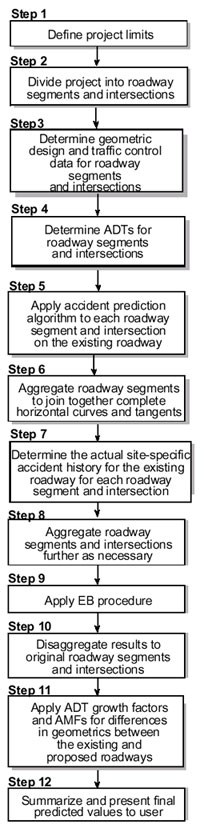
Figure 6. Flow Diagram of the Accident Prediction Algorithm When Site-Specific History Data Are Available.
Step 2—Divide the project into individual homogeneous roadway segments and intersections
The next step is to divide the project into individual homogeneous roadway segments and intersections. The roadway must be divided into homogeneous segments. A new homogeneous segment begins at each intersection where the value of one of the following variables changes:
- Average daily traffic volume (veh/day).
- Lane width.
- Shoulder width.
- Shoulder type.
- Driveway density (driveways per mile).
- Roadside hazard rating.
Also, a new analysis section starts at any of the following locations:
- Intersection.
- Beginning or end of a horizontal curve.
- Point of vertical intersection (PVI) for a crest vertical curve, a sag vertical curve, or an angle point at which two different roadway grades meet.
- Beginning or end of a passing lane or short four-lane section provided for the purpose of increasing passing opportunities.
- Beginning or end of a center two-way left-turn lane.
This segmentation process is applied to both the existing (before period) roadway and the proposed (after period) roadway. Each station that represents a division point for either the existing or proposed roadway must be used as the beginning point of anew segment for purposes of the analysis. In addition, each intersection is treated as a separate entity for analysis.
Step 3—Determine the geometric design and traffic control features for each individual roadway segment and intersection for both the existing and proposed roadway.
For each roadway segment, the following geometric and traffic control features must be quantified for both the existing and proposed roadways:
- Length of segment (mi).
- ADT (veh/day).
- Lane width (ft).
- Shoulder width (ft).
- Shoulder type (paved/gravel/composite/turf).
- Presence or absence of horizontal curve (curve/tangent).
- Length of horizontal curve (mi), if the segment is located on a curve. [This represents the total length of the horizontal curve, even if the curve extends beyond the limits of the roadway segment being analyzed.]
- Radius of horizontal curve (ft), if the segment is located on a curve.
- Presence or absence of spiral transition curve, if the segment is located on a curve. [This represents the presence or absence of a spiral transition curve at the beginning and end of the horizontal curve, even if the beginning and/or end of the horizontal curve are beyond the limits of the segment being analyzed.]
- Superelevation of horizontal curve, if the segment is located on a horizontal curve.
- Grade (percent), considering each grade as a straight grade from PVI to PVI (i.e., ignoring the presence of vertical curves).
- Driveway density (driveways per mi).
- Presence or absence of a passing lane to increase passing opportunities.
- Presence or absence of a short four-lane section to increase passing opportunities.
- Presence or absence of a two-way left-turn lane.
- Roadside hazard rating.
For each intersection, the following geometric and traffic control features must be quantified for both the existing and proposed roadways:
- Number of intersection legs (3 or 4).
- Type of traffic control (minor-road STOP, all-way STOP, minor-road YIELD control, or signal).
- Intersection skew angle (degrees departure from 90 degrees, with a + or - sign indicating the direction of the departure).
- Number of major-road approaches with intersection left-turn lanes (0, 1, or 2).
- Number of major-road approaches with intersection right-turn lanes (0, 1, or 2).
- Number of intersection quadrants with deficient intersection sight distance (0, 1, 2, 3, or 4).
The values of these geometric and traffic control parameters for roadway segments and intersections, for both the existing and proposed designs, will be determined from the CAD system, from existing data files for those designs, or from data supplied by the user.
Step 4—Determine the ADTs for each roadway segment and the major- and minor-road ADTs for each intersection during each year of the before period for which observed accident history data are available and for each year of the after period for which the expected safety performance is to be predicted.
For each roadway segment and for the major- and minor-road approaches to each intersection, ADT data are needed for each year of the before-and-after periods. Ideally, these ADT data will already be available in a file or they will be entered by the user. If ADTs are available for every roadway segment, the major-road ADTs for intersection approaches can be determined without additional data being supplied by the user. If the ADTs on the two major-road legs of an intersection differ, the average of the two ADT values should be used for the intersection. For a three-leg intersection, the user should enter the ADT of the minor-road leg. For a four-leg intersection, the user should enter the average of the ADTs for the two minor-road legs.
In many cases, it is expected that ADT data will not be available for all years of the before or after period. In that case, the analyst should interpolate or extrapolate as appropriate to obtain an estimate of ADT for each year of the evaluation period. If the analyst does not do this, the following default rules are applied within the accident prediction algorithm to estimate the ADTs for years for which the data are not available. If ADT data are available for only a single year of the before period, that same value is assumed to apply to all years of the before period. If two or more years of ADT data for the before period are available, the ADTs for intervening years is computed by interpolation. ADTs for years before the first year for which data are available are assumed to be equal to the ADT for that first year; ADTs for years after the last year for which data are available should be assumed to be equal to the last year (i.e., no extrapolation is used by the algorithm). The same approach should be used to determine ADT data for the after period.
Step 5—Apply the accident prediction algorithm to each of the individual roadway segments and intersections that make up the existing roadway.
The accident prediction algorithm should be applied to each individual roadway segment and intersection that makes up the existing roadway. This step is equivalent to steps 5 through 12 of the algorithm applied when site-specific accident data are not available, as presented earlier in this section of the report. The accident prediction algorithm is applied to roadway segments using equation (13), which incorporates the base model in equation (6), the calibration factor for roadway segments, and the roadway segment AMFs. The accident prediction algorithm for intersections is applied using equation (14), which incorporates the base models in equations (8), (10), or (12), depending on the type of intersection being evaluated, the calibration factor for intersections, and the intersection AMFs. The accident prediction algorithm is applied to each roadway segment or intersection individually for each year of the before period, using the appropriate ADT(s) for that year, and the results for that segment or intersection are summed over all the years to obtain a total predicted accident frequency for the before period. The total predicted accident frequency is allocated to two severity levels (fatal or injury accidents and PDO accidents) based on default proportions from table 1 in the main text of this report.
The predicted accident frequencies obtained from this process are designated Nrs for a roadway segment, Ni1 for a three-leg STOP-controlled intersection, Ni2 for a four-leg STOP-controlled intersection, and Ni3 for a four-leg signalized intersection. Each of these predicted frequencies has associated with it predicted frequencies by severity level that sum to the predicted total accident frequency.
Step 6—Aggregate roadway segments to join together complete horizontal curve and tangent sections.
The individual roadway segments are often so short, and have so few predicted and observed accidents, that it would not be meaningful to apply the EB procedure to each individual roadway segment. Therefore, aggregation of short roadway segments into longer segments, which will be called EB analysis units, is desirable.
The first stage of this process is to joint together complete horizontal curve and tangent sections of roadway. Proceed in geographical order from one end of the project (e.g., in order of increasing centerline stations) and join roadway segments together leaving breaks between segments only at the following locations:
- Intersections.
- Other points at which the ADT changes by 20 percent or more.
- Beginnings and ends of horizontal curves.
- Beginnings and ends of grades of 5 percent or more that fall with a tangent roadway section.
- Beginnings and ends of passing lanes.
- Beginnings and ends of short, four-lane sections.
- Beginnings and ends of two-way left-turn lanes.
As the segments are aggregated, their predicted accident frequencies (total and for each severity level) should be added together.
Step 6 deals only with the aggregation of roadway segments. For the present, each individual intersection serves as a separate EB analysis unit.
Step 7—Determine the observed accident history during the before period for each of the aggregated roadway segments from step 6 and for each intersection. If accident locations are not available in sufficient detail to identify the individual accident history for each aggregated roadway section and each intersection, aggregate roadway sections and/or intersections further, as necessary, until EB analysis units are obtained for which observed accident frequencies can be determined.
The observed accident history for the before period is obtained from one of two sources: (1) an available accident data file available that can be queried on-line; or (2) key entry of accident data for individual EB analysis units by the IHSDM user. If an accident history file is used, the user will have supply data on the correspondence between the accident location system used in the file (e.g., mileposts) and the stationing system used for the project. This can consist, for example, of the milepost corresponding to the end of the project with the lowest station and an indication of whether mileposts and stations increase in the same direction or in opposite directions. Then, the accident prediction algorithm can calculate the milepost limits of each aggregated roadway segment and the milepost of each intersection and retrieve accident data for each. Intersection-related accidents with 76 m (250 ft) of the intersection should be attributed to that intersection. Non-intersection-related accidents and intersection-related accidents that are located more than 76 m (250 ft) from an intersection should be attributed to the roadway segment within which the accident falls. It should be noted that there are very few intersection-related accidents more than 76 m (250 ft) from an intersection on rural two-lane highways. Intersection-related and non-intersection-related accidents can be distinguished in accident data from most states by the investigating officer’s assessment of whether a given accident was intersection related. The available accident file should be used to determine both total observed accidents and accidents by severity level.
If no accident file is available, the accident prediction algorithm will prompt the user to supply total accidents and accidents by severity level for each roadway segment (identified by a range of centerline stations) and each intersection (identified by station and, if possible, by the name of the intersecting minor road). For a large project, this data entry may be tedious, so it will be advantageous to have a accident file whenever possible.
If accident locations are not available in sufficient detail to identify the individual accident history for each aggregated roadway section and each intersection, it will be necessary to aggregate roadway sections and/or intersections further, as necessary, until EB analysis units are obtained for which observed accident frequencies can be determined. The IHSDM user will be asked to identify situations in which further aggregation is necessary because of limitations in the availability or precision of accident locations. Roadway segments and intersections and intersections of different types can be joined together, if necessary, if the accident histories of roadway segments and intersections, or the accident histories of closely-spaced intersections, cannot be distinguished. If the available accident data consist only of totals at the project level, then the entire project can be aggregated into one EB analysis unit, although this should be done only if necessary.
The observed accident frequencies for the before period for a given analysis unit are designated Ors for a roadway segment, Oi1 for a three-leg STOP-controlled intersection, Oi2 for a four-leg STOP-controlled intersection, and Oi3 for a four-leg signalized intersection. Each of these observed frequencies has associated with it observed frequencies by severity level that sum to the observed total accident frequency.
Step 8—Aggregate roadway segments and/or intersection further, if necessary, into larger EB analysis units to ensure a minimum accident sample size for each analysis unit.
It is desirable for an EB analysis unit (i.e., an aggregated roadway segment, an intersection or intersections of a specific type, a combination of roadway segments and intersections, or a combination of intersections of different types) to have at least a minimum number of predicted accidents for the EB procedure to be applied as intended. An individual roadway segment or intersection can constitute an EB analysis unit (i.e., can be evaluated by itself in the EB procedure) if observed accident history data are available for the analysis unit and the accident frequency predicted by the model for the before period is equal to at least 1/k, where k is the overdispersion parameter of the relevant base model. Table 23 shows the desirable minimum numbers of predicted accidents for application of the EB procedure to roadway segments and each type of intersection.
The predicted injury accident frequencies for EB analysis units after any further aggregation in step 7 should be reviewed to determine if there are any analysis units for which the predicted injury accident frequency is less than 1/k, based on table 23. If roadway segments and intersections or intersections of different types are mixed together, use the value of largest appropriate value of 1/k from table 23 for purposes of step 8 (a more sophisticated procedure for dealing with disparate k values will be used in step 9). Any EB analysis unit for which the predicted accident frequency is less than 1/k is a candidate for further aggregation.
Since, an EB analysis unit can combine roadway segments and intersections of different types, its total predicted accident frequency is the sum of the predicted accident frequencies of its constituent segments and intersections:
| N = Nrs + Ni1 + Ni2 + Ni3 |
(39)
|
where:
| Ni1 |
= |
predicted accident frequency for three-leg STOP-controlled intersections; |
| Ni2 |
= |
predicted accident frequency for four-leg STOP-controlled intersections; and |
| Ni3 |
= |
predicted accident frequency for four-leg signalized intersections. |
Similarly, the total observed accident frequency for an EB analysis unit is the sum of Ors, Oi1, Oi2,and Oi3.
The aggregation process is conducted as follows:
Step 8A—Select as candidates for further aggregation all analysis units consisting exclusively of tangent roadway segments with grades less than 5 percent for which the predicted injury accident frequency is less than 1/k.
Step 8B—For each of the candidate analysis units, compute the ratio of the predicted total accident frequency to the observed total accident frequency [i.e., N/O, or (Nrs+Ni1+Ni2+Ni3)/(Ors+Oi1+Oi2+Oi3)].
Step 8C—Select the candidate with the lowest predicted accident frequency. If no more candidates remain, go to step 8F.
Step 8D—Identify and select another candidate whose ratio of predicted to total accident frequency is closest to that of the candidate selected in step 8C. The two selected candidate do not necessarily need to be geographically adjacent. If there are no remaining candidates other than the candidate selected in step 8C, then select the analysis unit of the same type (i.e., a tangent roadway segment with grades less than 5 percent) with predicted injury accident frequency greater or equal to 1/k whose ratio of predicted to total accident frequency is closest to that of the selected candidate. If there are no eligible analysis units, including even those with predicted injury accident frequency greater than 1/k, proceed to step 8F.
Step 8E—Combine the analysis unit selected in step 8C with the analysis unit selected in step 8D, add together their predicted and observed accident frequencies (i.e., sum the values of Nrs, Ni1, Ni2, Ni3, Ors, Oi1, Oi2, and Oi3, for total accidents and by accident severity level), and recompute the ratio of predicted and observed total accident frequency. If the predicted injury accident frequency for the combined section is greater than 1/k, then go to step 8F. If the predicted injury accident frequency is still less than 1/k, then go back to step 8D and identify another section to combine.
Step 8F—Repeat steps 8A through 8E for each of the following types of analysis units, in turn:
- Tangent segments with grades greater than or equal to 5 percent.
- Horizontal curve segments.
- Tangent segments with grades less than 5 percent in passing lanes.
- Tangent segments with grades greater than or equal to 5 percent in passing lanes.
- Horizontal curve segments in passing lanes.
- Tangent segments with grades less than 5 percent in short four-lane sections.
- Tangent segments with grades greater than or equal to 5 percent in short four-lane sections.
- Horizontal curve segments in short four-lane sections.
- Tangent segments with grades less than 5 percent in two-way left-turn lanes.
- Tangent segments with grades greater than or equal to 5 percent in two-way left-turn lanes.
- Horizontal curve segments in two-way left-turn lanes.
- Three-leg STOP-controlled intersections.
- Four-leg STOP-controlled intersections.
- Four-leg signalized intersections.
Step 8G—If analysis units with predicted injury accident frequency less than 1/k remain, repeat steps 8A through 8E joining together analysis units of disparate types in the following order of descending priority:
- Join tangent roadway segments of any type to other tangent roadway segments of any type.
- Join horizontal curve segments of any type to horizontal curve segments of any type.
- Join three-leg STOP-controlled intersections to other three-leg STOP-controlled intersections.
- Join four-leg STOP-controlled intersections to other four-leg STOP-controlled intersections.
- Join four-leg signalized intersections to other four-leg signalized intersections.
- Joint tangent roadway segments with horizontal curves.
- Join three-leg STOP-controlled intersections to four-leg STOP-controlled intersections.
- Join signalized intersection with STOP-controlled intersections.
- Join roadway segments and intersections.
The aggregation process can be stopped whenever no analysis units with predicted injury accident frequency less than 1/k remain or whenever the entire project has been joined into a single analysis unit.
Step 9—For each EB analysis unit, as joined in Step 8, apply the EB procedure by computing the expected accident frequency for the before period as a weighted average of the predicted and observed accident frequencies.
The next step is to apply the EB procedure by computing a weighted average of the predicted and observed accident frequencies for the before period. For any EB analysis unit that is composed of entirely of roadway segments or composed entirely of a single intersection type, compute the weight to be placed on predicted accident frequency using equation (33) and then compute the expected accident frequency using equation (32).
If an EB analysis unit combines roadway segments and intersections, or more than one type of intersection, two additional factors must be accounted for. First, the overdispersion parameter, k, in the denominator of equation (33) is no longer uniquely defined, because two or more base models with differing overdispersion parameters must be considered. Second, it can no longer be assumed, as is normally done, that the expected numbers of accidents for the roadway segments and intersections, or for the different types of intersections are statistically correlated with one another. Rather, an estimate of expected accidents should be computed based on the assumption that the different entities are statistically independent (r=0) and on the alternative assumption that they are perfectly correlated (r=1). The expected accident frequency is then estimated as the average of the estimates for r=0 and r=1. This approach is implemented with equations (34) through (38).
Step 9 is applied both to predicted and observed total accident frequencies and to predicted and observed accident frequencies by accident severity level. Since these computations are independent, the expected accident frequencies by severity level may not sum to the expected total accident frequency. A correction is made as follows so that the expected accident frequencies for the individual severity levels do sum to the expected total accident frequency:
| Efi/corr = |
Etot
|
 |
Efi
|
|
(40)
|
|
|
Efi + Epdo
|
| Epdo/corr = |
Etot
|
|
Epdo
|
|
(41)
|
|
|
Efi + Epdo
|
where:
| Efi/corr |
= |
expected accident frequency for fatal and injury accidents (corrected); |
| Epdo |
= |
expected accident frequency for property-damage-only accidents (corrected); |
| Etot |
= |
expected accident frequency for total accidents as estimated with equations (34) to (38); |
| Efi |
= |
expected accident frequency for fatal and injury accidents as estimated with equations (34) to (38); and |
| Epdo |
= |
expected accident frequency for property-damage-only accidents as estimated with equations (34) to (38). |
Step 10—For each EB analysis unit, disaggregate the expected total accident experience during the before period back to the original roadway segments and intersections identified in step 2.
If an EB analysis unit, consists of more than one roadway segment or intersection, the expected accident frequency (Nxx) for the EB analysis unit should be disaggegated back to the original roadway segments and intersections in proportion to their original predicted accident frequencies. In other words:
|
Ep =
|
Eau
|
|
Np
|
|
(42)
|
|
|
Nau
|
where:
| Ep |
= |
expected accident frequency for an individual homogeneous roadway segment or intersection; |
| Eau |
= |
expected accident frequency for an EB analysis unit combining two or more roadway segments or intersections; |
| Np |
= |
original predicted accident frequency for the individual homogeneous roadway segment or intersection from step 5; |
| Nau |
= |
original predicted accident frequency for all roadway segments and intersections that make up the analysis unit, as aggregated in steps 6 and 8. |
Repeat this process for each of the original roadway segments and intersections, for total accidents and for each severity level.
Step 11—Apply ADT growth factors and/or AMFs for geometric changes to convert the expected accident frequency for the before period to an expected accident frequency for the proposed project during the specified future time period.
At the conclusion of step 10, Ep represents the expected accident frequency for a given roadway segment or intersection during the before period. To obtain an estimate of expected accident frequency in a future period (the after period), the estimate must be corrected for (1) any difference in the duration of the before-and-after periods; (2) any growth or decline in ADTs between the before-and-after periods; and (3) any changes in geometric design or traffic control features between the before-and-after periods that affect the values of the AMFs for the roadway segment or intersection. The expected accident frequency for a roadway segment or intersection in the after period can be estimated as:
| Ef = Ep (Nbf / Nbp) (AMF1f / AMF1p) (AMF2f / AMF2p) ... (AMFnf / AMFnp) |
(43)
|
where:
| Ef |
= |
expected accident frequency during the future time period for which accidents are being forecast for the analysis segment or intersection in question; |
| Ep |
= |
expected accident frequency for the past time period for which accident history data were available; |
| Nbf |
= |
number of accidents forecast by the base model using the future ADT data, the specified nominal values for geometric parameters, and—in the case of an analysis segment—the actual length of the analysis segment; |
| Nbp |
= |
number of accidents forecast by the base model using the past ADT data, the specified nominal values for geometric parameters, and—in the case of an analysis segment—the actual length of the analysis segment; |
| AMFxf |
= |
value of the xth AMF for the geometric conditions planned for the future (i.e., proposed) design; and |
| AMFxp |
= |
value of the xth AMF for the geometric conditions for the past (i.e., existing) design. |
Because of the form of the base model for roadway segments, the ratio Nbf / Nbp is the same as the ratio of the traffic volumes, ADTf / ADTp. However, for intersections, the ratio Nbf / Nbp must be evaluated explicitly with the base models because the intersection base models incorporate separate major- and minor-road ADT terms with differing coefficients. In applying equation (43), the values of Nbp, Nbf, AMFxp, and AMFxf should be based on the average ADTs during the entire before or after period, respectively.
Equation (43) is applied to total accident frequency. The expected future accident frequencies by severity level should also be determined by multiplying the expected accident frequency from the before period for each severity level by the ratio Ef/Ep.
In the case of minor changes in roadway alignment (i.e., flattening a horizontal curve), the length of an analysis segment may change from the past to the future time period. In this case, the length of the analysis segment for the existing condition is used to determine Nbp and the modified length of the analysis segment for the planned condition is used to determine Nbf. This implicitly incorporates the assumption that, if the length of the analysis segment is changed, its base accident rate (per million-vehicle miles) remains constant and, therefore, the accident frequency increases or decreases in proportion to length. Of the course, the AMF ratios that also appear in equation (43) will account for any change in geometrics (i.e., reduction in radius of curvature) that accompany a change in length.
Step 12—Summarize and present the predictions in useful formats for the IHSDM user.
In the final step, the predicted accident frequencies are summarized and presented in useful formats for IHSDM users. The data presented include, at a minimum:
- Accident frequencies for the project as a whole including:
-- Total accident frequency.
-- Accident frequency by severity level.
-- Accident frequency by accident type.
The accident severity and accident type distribution for each roadway segment and intersection in the specified future time period is based on the default accident severity and accident type distributions presented in tables 1 and 2.
- Accident frequencies for individual roadway segments and intersections, expressed as accident rates per mi per year or million veh-mi for roadway segments and accident rates per million entering vehicles for intersections, so that accident “hot spots” that might be corrected through design improvements are evident
Estimated accident frequencies could also be broken down by individual years of the evaluation period. However, this is not normally done because the combined estimates across all years of the evaluation period are generally of greatest interest to safety analysts. Predicted accident frequencies for a multiyear period are likely to be more accurate than predicted accident frequencies for any particular year.
Previous | Table of Contents | Next
|


