U.S. Department of Transportation
Federal Highway Administration
1200 New Jersey Avenue, SE
Washington, DC 20590
202-366-4000
Federal Highway Administration Research and Technology
Coordinating, Developing, and Delivering Highway Transportation Innovations
 |
| This report is an archived publication and may contain dated technical, contact, and link information |
|
Publication Number: FHWA-HRT-04-140
Date: December 2005 |
||||||||||||||||||||||||||||||||||||||||||||||||||||||||||||||||||||||||||||||||||||||||||||||||||||||||||||||||||||||||||||
Enhanced Night Visibility Series, Volume IX: Phase II—Characterization of Experimental ObjectsPDF Version (716 KB)
PDF files can be viewed with the Acrobat® Reader® CHAPTER 2—METHODSThe method in this experiment was used primarily for the investigation of the objects that were used in the ENV clear-condition visual performance study, which are fully documented in Volume III of this series. The effects of rain, snow, and fog conditions were also assessed, and these results are included after the analysis of the results for the clear weather condition. EXPERIMENTAL DESIGNThe experiment used a full-factorial design for the measurement process for both the object and VES data. In total, 8 of the objects and 11 of the VESs compared in the ENV clear-condition study were also used in this experiment. The factorial format in this experiment was an 8 (Object Type) by 11 (VES Configuration) by 6 (Station) by 4 (Measurement Distances) design with the conditions shown in table 1.
Within each of these variables, the levels were selected to match those of the ENV Phase II visual performance experiments. Independent VariablesObject TypeThe objects varied in both color and position relative to the roadway. Table 2 outlines the objects used in this study and the objects they represented from the ENV clear-condition study. It should be noted that the objects used for this investigation were all static, but most of the objects in the ENV clear-condition study were dynamic. The characterization used static objects because the measurement process was lengthy, requiring that the objects be still during the process. This also meant that the white-clothed static pedestrian and white-clothed parallel pedestrian from the ENV clear-condition study were characterized as the same object in this investigation.
VESFour different vehicles were used to provide the 11 different VESs used in the characterization activity. During the visual performance studies, participants drove a vehicle on the Virginia Smart Road and announced when they could detect and identify the objects of interest. After the participant completed a lap of the Smart Road, the VES was changed to the next configuration. This process might have required the participant to change vehicles. The VES types used are shown in table 3. Again, the IR–TIS VES from the Phase II studies was not included in this characterization effort.
The headlamps used for the HLB, HID, HOH, HHB, and UV–A configurations were located on external light bars. To change from one configuration to another, the HLB and HID headlamps were moved onto, off of, and between vehicles. Each light assembly movement required a re-aiming process, which took place before starting the experimental session each night. At the beginning of the Phase II studies, a headlamp aimer was not available to the contractor, so an aiming protocol was developed with the help of experts in the field. During the photometric characterization of the headlamps, it was discovered that the maximum intensity location of the HLB, HOH, and HHB configurations was aimed higher and more toward the left than typical. This aiming method may have influenced the visual performance testing results; however, this object characterization process evaluates the objects as they were presented to the experimental participants. Details about the aiming procedure and the maximum intensity location are discussed in ENV Volume XVII, Characterization of Experimental Vision Enhancement Systems. StationDuring the ENV visual performance experiments, the objects appeared randomly at one of six stations (locations) identified on the Smart Road. These stations were defined by distance from the start point of the lap (figure 1). There were three downhill stations and three uphill stations, relative to the travel direction of the experimental vehicle during a lap. As the participant drove the experimental lap on the road, objects were presented at the various stations; sometimes no objects were presented in order to reduce participant expectancy. Not all objects were used at each location. Table 4 summarizes the stations and objects presented. 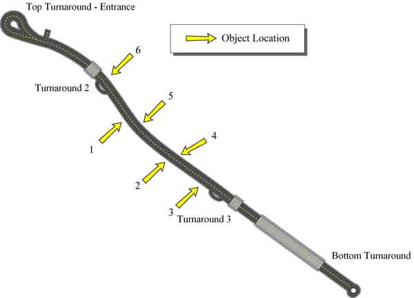 Figure 1. Diagram. Object stations (locations) on the Virginia Smart Road.
The object luminance was determined at two stations, one uphill and one downhill (station 4 and station 2). The object background luminance was established at all stations. The luminance of the objects was measured through the rain at station 2, called station R2 for this condition, to characterize the effect of rain on object visibility. DistanceThe distance from an observer to an object is also a factor in the evaluation of object visibility, affecting its visual size and the illuminance on the object. The location from which to perform the photometric characterization was determined by the closest distance of the participant vehicle to the object during the ENV visual performance experiments. The safety protocol of the Phase II experiments had directed the experimenters who stood as objects to clear the roadway when the participant vehicle was within 61.0 m (200 ft) of the station; therefore, this distance to the object became the basis for headlamp illuminance, object luminance, and background luminance measurement distances for all VES types and objects. To more fully establish the effect of distance on visibility, object luminance, background luminance, and illuminance measurements were made at 91.5 m (300 ft), 152.5 m (500 ft), and 244 m (800 ft). Because the illuminance falls off with the square of the distance, only the white-clothed pedestrian objects were measured at these longer distances to provide the highest possible luminance of the objects, and consequently, the lowest measurement uncertainty. These measurements were made at only two of the six stations (i.e., stations 2 and 4), and the results were then applied to all stations and object types. Because the background changed among stations, background luminance measurements were made at all of the stations from a distance of 61.0 m (200 ft). Because UV–A radiation did not change the background luminance, only the contributing non-UV–A VESs were measured at these points. Table 5 summarizes the components of the measurement process.
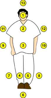
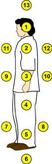
The final aspect of the experimental design was the weather condition. During the ENV visual performance experiments, participants were presented with the objects in rain, fog, snow, and clear conditions. The weather conditions were re-created on the Smart Road using its all-weather testing capabilities. For the object characterization, measurements to calculate atmospheric transmittance were made in all of these weather conditions. Based on this calculation, it is possible to develop factors accounting for the effect of weather on the object photometric characteristics. More information about the measurement procedures and results appear in chapter 5 of this document. Dependent VariablesThe object luminance, background luminance, and illuminance from the VES are the dependent variables in this experiment. Other calculated characteristics are discussed as part of the data analysis. Object and Background LuminanceFor each object, a series of as many as 14 luminance measurements were made including measurements of both the background and object itself. Figure 2 and figure 3 show the measurement points for the two pedestrian object types.
The numbers in the circles indicate the measurement point number. For the analysis, the measurement points were separated into groups, object (1 through 5) and background (6 through 13), and replaced with height and positions. This means that measurement point 3 was converted to waist height, and measurement points 9 and 10 were converted to waist-left and waist-right measurements. This was performed for the analysis so that measurements at the same height could be compared. For the black-clothed and white-clothed cyclist conditions, the measurement points were very similar to those of the pedestrians, but the face measurement was removed from the group because it was the same regardless of the VES or object clothing. Two measurement points were added to the bicycles themselves (i.e., points 5 and 6). These were on the wheel rims because they were the brightest parts of the bicycles. Figure 4 shows the cyclist measurement points. 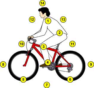 Figure 4. Illustration. Cyclist measurement points.
For the child’s bicycle, two measurements were made of the frame (points 1 and 2), and four were made of the background (points 3 through 6). As with the pedestrian objects, the measurements of all objects were separated into object and background measures for analysis. Figure 5 outlines the measurements taken for the child’s bicycle when it was lying horizontally. 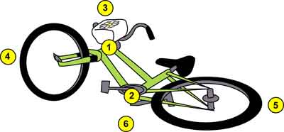 Figure 5. Illustration. Child’s bicycle measurement points.
The tire tread was similar; however, this object was measured only once (point 1), and the background was measured around it (points 2 through 5). Figure 6 shows the measurement points on the tire tread. 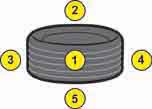 Figure 6. Illustration. Tire tread measurement points.
For measurements at stations where the background was the only measurement series of interest (stations 1, 3, 5, and 6), the object was placed at the location to ensure that the same background measurement points were used. VES IlluminanceThe illuminance falling on the objects, provided by the VESs, was measured for each object type. For the human objects, the vertical illuminance was measured at seven points. The first four points were on parts of the objects facing the vehicle and corresponding to the luminance measurement heights of chest, waist, knee, or ankle. The next three points, one at chest height on either side of the object and one behind it, were used to measure the ambient illuminance falling on each side of the object. The illuminances on the child’s bicycle and the tire tread were measured at the same points as those objects’ luminance measurements. APPARATUSThe measurement apparatus used for this experiment were a photometer and an illuminance meter. The same object materials (pedestrian surgical scrubs, bicycles, tire treads) used in the ENV visual performance studies were used for the characterization. The photometric measurements were made using a Model 1980A Pritchard® Telephotometer on loan from the Federal Highway Administration. The telephotometer provides five measurement apertures ranging from 2′ to 3°. During the experiment, the 6′ aperture was used for all measurements made at 61.0 m (200 ft). The 2′ aperture was used for measurements made at longer distances. The minimum sensitivities of the photometer with the 6′ and 2′ apertures are 3×10⁻² candela per square meter (cd/m²) and 3×10⁻¹ cd/m² respectively. The uncertainty associated with the telephotometer is ±4 percent of the measurement. The illuminance meter used in the experiments was a Konica Minolta® T-10. The minimum sensitivity provided by this instrument is 0.01 lux (lx) with an uncertainty of ±2 percent of the most significant digit; however, the meter does have an 8 percent f1′ factor. This means that the sensitivity of the detector can deviate from the response of the human eye by as much as 8 percent depending on the light source being measured. Because most of the VES types were incandescent-halogen based, the illuminance meter was calibrated with a Commission Internationale de l’Eclairage Standard Illuminant A. Consequently, measurements of HID VESs had a slightly higher uncertainty. TESTING PROCEDUREThe testing took place on the Virginia Smart Road test facility. For each VES, the telephotometer was placed in the driver’s seat of the test vehicle. A photometer operator who sat in the rear seat of the vehicle aimed the photometer at the objects. An additional experimenter sat in the front seat of the vehicle and recorded the results. This differed from the ENV visual performance studies, in which the participant and an experimenter both sat in the front seats of the experimental vehicle. In a typical testing process, all of the measurements were performed in a series at each station, with the measurement of one object followed by the measurement of the next object until all of the objects for that station had been tested with that VES. The next step was to change the VES on the vehicle and test all of the objects with it. After all of the VESs available on one vehicle were tested, the photometer was moved to the next vehicle, until all VESs were tested. Care was taken to ensure that the warmup time and stabilization of both the photometer and the VES matched to avoid inconsistencies between conditions. After all of the objects and VES conditions were tested at a station, the setup moved to the next station, and the process continued. As mentioned, the number and seating arrangement of vehicle occupants in the test condition differed from the configuration in the ENV detection testing. This means that the vehicle’s weight distribution was not the same between the test processes of the ENV detection studies and the photometric characterization. A short comparison test was performed to investigate how the photometer operator’s position affected the measurements; these measurements were for this comparison only, and they were not included in the experimental design. For this set of data, the object and background luminance measurements were performed with the photometer operator sitting in the back seat of the vehicle, just as it was performed in the characterization activity. Then the measurements were taken again with the photometer operator sitting in the driver’s seat of the vehicle; the photometer’s tripod was placed in the photometer operator’s lap. The measurements were made at the 244-m (800-ft) distance because it would show the greatest change resulting from the front-to-back tilt in the vehicle. The measurements were taken with the test vehicle pointed uphill toward station 4. Only the WPP, WPL, and WC objects were used for these comparisons. The VESs used were limited to the HLB, three UV–A + HLB, and five UV–A + HLB. The photometric results from the two positions were then compared using their means and standard errors. The results for all of the measurements are seen in figure 7 for each of the UV systems. Figure 7 comprises the mean of the background and object luminance data for all objects from both of the photometer operator’s positions. This figure shows that the two photometer operator positions yielded similar measurements. 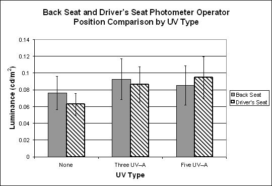 Figure 7. Bar graph. Comparison of the mean of background object luminance for
HLB combined with different UV–A levels when the photometer operator is in the back seat or the driver’s seat. To further review these results, the data for the object luminance were considered separately because these data were more likely to have been affected by the change in the tilt of the vehicle than the background luminance data. The bar graph in figure 8 shows a slight difference between the object measurements for the two positions of the photometer operator for the HLB VES; however, there was no such significant difference for the HLB VESs with UV–A. From this data, it can be seen that the standard error associated with the measurements was greater than any difference produced by the position of the photometer operator. Based on this analysis, it was decided that the measurement procedure with the photometer operator in the back seat of the vehicle was valid, and the position did not influence the measurement results. 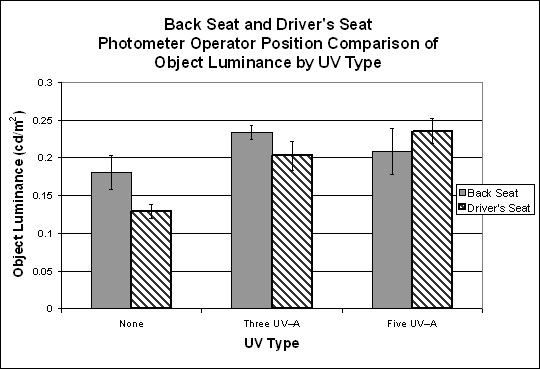 Figure 8. Bar graph. Comparison of object luminance for HLB combined with different
UV–A levels when the photometer operator is in the back seat or the driver’s seat. DATA ANALYSISThe dependent variables measured on the Smart Road were used to derive several other metrics, namely the object reflectivity, object fluorescence, contrast, and visibility level. ReflectivityThe reflectivity of the object can be calculated using the assumption that the object of interest is a Lambertian (diffuse in all directions) reflector. If this assumption is made, the reflectivity is calculated from the incident illuminance and the object luminance. This is determined through the equation shown in figure 9. Figure 9. Equation. Lambertian reflection.
In this equation, Some objects in this study did not reflect diffusely, but rather, they acted specularly. These were the shiny objects such as certain parts of the bicycles. This means that reflectivity has a directional component, and thus the Lambertian assumption is not valid. For such objects, the specular reflectivity in a given direction is calculated using the equation in figure 10. Figure 10. Equation. Specular reflection.
In both cases, the reflectivity is a ratio usually expressed in percent, and it does not have specific units. It is important to note that the reflectivity of the objects can be established only for the non-UV–A containing VESs. If the UV–A containing VESs are used, the measured luminance contains both the reflected light and the light generated through the fluorescence of the clothing material and possibly the paint on the bicycle used in the cyclist conditions and the child’s bicycle. FluorescenceThe contribution of the UV–A to the appearance of the material can be assessed by examining the increase in the object’s luminance with the various UV–A VES configurations. To establish the fluorescence of the material, the reflectance of all of the object and VES combinations was calculated. These combinations included VESs with a UV–A component. The reflectance with these UV–A combinations could be much greater than 100 percent because the luminance was generated not only from the reflected visible light but also from the emitted fluorescence due to the UV. The fluorescence was calculated as the ratio of the object reflectance in a UV–A condition to that of the same object in a non-UV–A condition with the same visible-light headlamps. Figure 11 shows this relationship. Figure 11. Equation. Object fluorescence.
The equation in figure 11 assumes that the UV–A reflectance will always be greater than the non-UV–A reflectivity. This relationship established the fluorescent activation capability of each of the object types and each of the VESs. Note, a %Fluorescence value of 100 percent indicates no increase in the object’s luminance with the various UV–A VES configurations. ContrastThe contrast of the object to the background can be expressed as the simple difference between the luminance of the object and the luminance of the background or as a ratio of the object and background luminance difference to the background luminance as shown in figure 12. Figure 12. Equation. Contrast ratio.
When the object is darker than the background, the relationship is negative; it is referred to as a “negative contrast condition.” In addition to the other analyses, the contrast of the human objects in the experiment was evaluated in two ways. The first was to use the average of the background measurements and the average of all of the object measurements in the contrast equation. The second was to evaluate the contrast at the various measurement heights (ankle, knee, waist, and chest) using the object measurement and the two corresponding (left, right) background measurements. This provided an idea of a contrast gradient on the object. The contrasts for the tire tread and the child’s bicycle were evaluated only as the average of the background versus the average of the object luminance measurement. Visibility LevelThe visibility level (VL) was calculated based on Adrian’s object visibility model, in which the threshold luminance difference ( The Adrian model is calculated using a basic formula with situational factors to modify the result for various conditions. The basic calculation is shown in the equation in figure 13.  Figure 13. Equation. Basic
The models for The basic Figure 14. Equation. Time factor for the
The function a( According to the Adrian model, targets that appear in negative contrast (i.e., object is darker than background) are more easily seen than those that appear in positive contrast (i.e., object is lighter than The final variable that must be accounted for is the age of the observer. The basic model was developed for a 23-year-old observer. To account for different age groups, a final factor was used. The format for the factor is shown in the equation in figure 15. Figure 15. Equation. Age factor for the
The value of the constants of a, b, and c are dependent on the age, and the values are presented in Adrian’s document. The final model of the  Figure 16. Equation. Complete
As a metric for visibility, the VL is the ratio of the actual luminance difference and Figure 17. Equation. Visibility level.
In this calculation, a VL of 1 would imply the detection threshold; however, in a driving task the threshold increases to allow for driver distraction and workload. Because there are no correction factors for driver distraction and workload, the Illuminating Engineering Society of North America RP-8-00 recommends that a VL of 2.6 to 3.8 be used in practice to account for those issues.(2) The Adrian model was used to calculate the VL of all of the objects used in this ENV object characterization. For this calculation, the observation time was set to 0.2 s. The target size was calculated based on the height of the object and the observation distance. The objects’ dimensions are summarized in table 6. A 99-percent detection confidence interval was used with a k factor of 2.9.
|