U.S. Department of Transportation
Federal Highway Administration
1200 New Jersey Avenue, SE
Washington, DC 20590
202-366-4000
Federal Highway Administration Research and Technology
Coordinating, Developing, and Delivering Highway Transportation Innovations
 |
| This report is an archived publication and may contain dated technical, contact, and link information |
|
Publication Number: FHWA-RD-02-045
Date: March 2003 |
||||||||||||||||||||||||||||||||||||||||||||||||||||||||||||||||||||||||||||||||||||||||||||||||||||||||||||||||||||||||||||||||||||||||||||||||||||||||||||||||||||||||||||||||||||||||||||||||||||||||||||||||||||||||||||||||||||||||||||||||||||||||||||||||||||||||||||||||||||||||||||||||||||||||||||||||||||||||||||||||||||||||||||||||||||||||||||||||||||||||||||||||||||||||||||||||||||||||||||||||||||||||||||||||||||||||||||||||||||||||||||||||||||||||||||||||||||||||||||||||||||||||||||||||||||||||||||||||||||||||||||||||||||||||||||||||||||
IHSDM Intersection Diagnostic Review Model3.0 IDRM MODELSAs discussed in Section 2.0 , IDRM evaluates the presence of potential concerns by applying engineering models to give a quantitative measure of an intersection's performance. The presence and level of a concern are determined by applying thresholds to one or more performance measures generated from the models. One model may be used to evaluate several concerns. This section documents the 21 models that were developed for the IDRM knowledge base. The models are summarized in Table 4 . The application of these models to the potential concerns evaluated by IDRM is summarized in Table 5 . Section 4.0 presents a detailed discussion of each potential concern and how the models are used to evaluate each concern. 3.1 Intersection Sight Distance for Case B1– Left Turn From Minor RoadApplicability An intersection sight distance (ISD) model for Case B1 is applied in IDRM wherever a driver may be stopped on the minor road awaiting an opportunity to complete a left-turn maneuver. Similar models for Cases B2, B3, and F are applied for a right-turn maneuver from the minor road, a crossing maneuver from the minor road, and a left-turn maneuver from the major road, respectively (see Sections 3.2 through 3.4 ). Basis Each stop-controlled intersection contains several potential vehicle conflicts. The possibility of these conflicts actually occurring can be greatly reduced through provision of the proper ISD. A driver approaching an intersection should have an unobstructed view of the entire intersection and, when stopped, sufficient lengths of the intersecting highway. The model used to determine the extent to which a driver can see an intersection is based on the ISD model used in geometric design, which has recently been modified in Intersection Sight Distance, NCHRP Report 383. The model, as developed in NCHRP Report 383 and presented in the 2001 AASHTO A Policy on Geometric Design of Highways and Streets (known as the Green Book), is:
where:
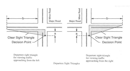
The available ISD, as limited by vertical geometry (ISDvert), is based on a driver's eye height (h1) of 1080 mm and an object height (h2) of 1080 mm. The driver's eye height (h1) should be adjusted for the profile of the minor road. The limitation of ISD due to the vertical alignment is determined as the maximum distance from the intersection that an object of height h2 can be seen from a driver's eye at height h1. The limitation of ISD due to horizontal alignment and roadside sight obstructions (including terrain, vegetation, man-made obstacles) is determined by evaluating whether particular sight triangles are clear of sight obstructions. Figure 2 illustrates the sight triangle used for ISD Case B1 (i.e., the ISD to the right for a left-turning vehicle). The other sight triangle shown in Figure 2 (i.e., the sight triangle to the left) is not explicitly considered by IDRM for Case B1. A left-turning driver does need sight distance to the left to cross the near lane of the major road in making a left turn, but the sight distance needed to cross the near lane of a two-lane highway (plus any adjacent left-turn lane) will always be less than or equal to the sight distance to the left for ISD Case B2 (right turn onto the major road) and ISD Case B3 crossing the major road; these cases are addressed below in Sections 3.2 and 3.3 , respectively.
Figure 2. Departure Sight Triangles for ISD Cases B1, B2, and B3 The major difference between the ISD model as it is applied in geometric design practice and the ISD model as it is applied in IDRM is that, in IDRM, the initial speed, V, is set equal to the actual 85th percentile speed of traffic in the roadway, Vact, or the best available estimate of Vact, rather than being set equal to a particular design speed. Input Parameters The input parameters used in the ISD model are:
The source of data for those input parameters whose values are not specified above are as follows:
Evaluation Procedure An ISD review procedure for the adequacy of sight distance for vehicles stopped on a minor-road approach will be formulated as follows: 1. Select a pair of major- and minor-road approaches to be evaluated. The ISD case to be examined is Case B1, Sight distance for a driver making a left turn (i.e., the minor-road driver must evaluate gaps in major-road traffic approaching from the left and from the right). 2. Determine Vact, the actual 85th percentile speed of traffic on the selected major-road approach. Vact can be determined from field data, from a speed prediction model like those developed for the IHSDM design consistency module, or from an engineering judgment by the user. The objective is to base the value of Vact, to the maximum possible extent, on actual field conditions rather than on an arbitrary design speed. 3. Select an appropriate time-gap value (tc) for evaluation of ISD. For application of IDRM to a passenger car driver, the recommended time-gap value for left turns is 7.5-s. This time gap is for traffic approaching from the right in the lane of the major road that is entered by the left-turning driver. As explained above, this 7.5 s time gap for ISD Case B1 is not applicable to traffic from the left in crossing the near lane of the major road. The time gap to cross the near lane will always be less than or equal to the gaps for sight distance to the left considered for ISD Cases B2 and B3 (see Sections 3.2 and 3.3, respectively). Based on NCHRP Report 383, an adjustment should also be made for the approach grade. If the approach grade on the minor road is an upgrade that exceeds 3 percent, add 0.2 s per percent grade to the time-gap value, tc. Otherwise, make no adjustment for the approach grade. 4. Compute several ISD measures as described below. The required ISD using the identified Vact and tc in the ISD model is determined with Equation 3.1.2:
For certain special situations where more complex geometrics place greater demands on drivers, the value of tc will be increased by an amount designated as Dt. This would result in Equation 3.1.2 being recast as:
The value for Dt may differ among the various intersection scenarios considered. Table 6 presents the values for Dt for each scenario. Values are recommended for skewed intersections and a horizontal curve on an intersection approach. Additional human factors studies will be needed to develop values for other scenarios. Table 6. Values of DT for Various Intersection Scenarios
The available ISD as limited by vertical geometry (ISDvert) is based on a driver's eye height (h1) of 1080 mm and an object height (h2) of 1080 mm. The driver's eye height (h1) should be adjusted for the profile of the minor road, in other words:
where:
Equation 3.1.4 assumes that the driver's eye is 4.4 m from the edge of the major-road traveled way as recommended in NCHRP Report 383. Where the full profile of the minor road is available, this should be used in determining Pminor as the average grade over a length 4.4 m from the edge of the major-road traveled way, which is shown as dimension a in Figure 2 . Thus, Pminor can be calculated as the elevation difference between the edge of the major-road traveled way and a point on the minor road 4.4 m from the edge of the major-road traveled way divided by the horizontal distance, 4.4 m. Where the full profile of the minor road is not available, Pminor should be assumed to be zero. ISDvert should be determined as the maximum distance from the intersection that an object of height h2 can be seen from a driver's eye at height h1. This criterion is applied along the centerline of the roadway, assuming that the driver's eye is located at a position LWminor/4 to the right of the center of the intersection. If ISDvert ³ ISDdes, then set ISDvert equal to ISDdes. This case occurs when there is no crest vertical curve within distance ISDdes from the intersection or when the crest is so slight that the driver can see over it. 5. Figure 2 illustrates the sight triangle used for ISD Case B1 to the right. The limitation of ISD due to the vertical alignment of the major road has been addressed above. The limitation of ISD due to horizontal alignment and roadside sight obstructions (including terrain, vegetation, man-made obstacles) should proceed by asking the user whether the particular sight triangles displayed by IDRM are clear of sight obstructions. This logic is specified as follows: If ISDvert > ISDdes, then display Figure 3 to the user with the query:
NOTE: In displaying Figure 3 to the user, the dimensions of the regions should be shown and the sight triangle should be drawn to scale and superimposed on an intersection plan view. The dimension of Region 1 along the major road is ISD1 (the equation for computing ISD1 is shown in Section 4.7). The dimension of Regions 1 and 2 combined along the major road is ISDvert. If the horizontal alignment of the major road is other than tangent, the curvilinear alignment of the major-road leg of the "triangle" must be displayed. The dimension of the leg of the sight triangle along the minor road is 4.4 m to the curb line plus the distance across the intersection to the mid point of the through lane on the far side of the road. 
Figure 3. Regions of the Sight Triangle for Which Users Will Be Queried About the Presence of Roadside Sight Obstructions 6. Proceed to consideration of the next pair of major- and minor-road approaches. Model Output The model output is the available intersection sight distance as limited by vertical geometry (ISDvert), the critical time gap (tc), and the user's response to whether the regions in Figure 3 are clear of roadside sight obstructions (YES/NO). The criticality of ISDdes is judged by comparison to ISDvert as described in Section 4. References
|
 |
Equation 3.2.1 |
where:
| ISD |
=
|
intersection sight distance (m) |
| V |
=
|
initial speed (km/h) |
| t |
=
|
driver perception-brake reaction time (s) |
The available ISD as limited by vertical geometry (ISDvert) is based on a driver's eye height (h1) of 1080 mm and an object height (h2) of 1080 mm. The driver's eye height (h1) should be adjusted for the profile of the minor road. The limitation of ISD due to the vertical alignment is determined as the maximum distance from the intersection that an object of height h2 can be seen from a driver's eye at height h1.
The limitation of ISD due to horizontal alignment and roadside sight obstructions (including terrain, vegetation, man-made obstacles) is determined by evaluating whether particular sight triangles are clear of sight obstructions. Figure 2 illustrates the sight triangle used for ISD to the left.
The major difference between the ISD model as it is applied in geometric design practice and the ISD model as it is applied in IDRM is that, in IDRM, the initial speed, V, is set equal to the actual 85th percentile speed of traffic in the roadway, Vact, or the best available estimate of Vact, rather than being set equal to a particular design speed.
Input Parameters
The input parameters used in the ISD model are:
| •Vact |
-
|
actual 85th percentile speed of traffic on the selected major road |
| •Pxslope |
-
|
cross-slope of the major-road pavement (%) |
| •LWmajor |
-
|
lane width of major road (m) |
| •Pminor |
-
|
grade of minor road (%) |
| •ADT |
-
|
average daily traffic volume (veh/day) |
The source of data for those input parameters whose values are not specified above are as follows:
| •Vact |
-
|
data file or user query |
| •Pxslope |
-
|
roadway file |
| •LWmajor |
-
|
roadway file |
| •Pminor |
-
|
roadway file |
Evaluation Procedure
An ISD review procedure for the adequacy of sight distance for vehicles stopped on a minor-road approach will be formulated as follows:
1. Select a pair of major- and minor-road approaches to be evaluated. The ISD case to be examined is Case B2, Sight distance for a driver making a right turn (i.e., the minor-road driver must evaluate gaps in major-road traffic approaching from the left).
2. Determine Vact, the actual 85th percentile speed of traffic on the selected major-road approach. Vact can be determined from field data, from a speed prediction model like those developed for the IHSDM design consistency module, or from an engineering judgment by the user. The objective is to base the value of Vact, to the maximum possible extent, on actual field conditions rather than on an arbitrary design speed.
3. Select an appropriate time-gap value (tc) for evaluation of ISD. For application of IDRM to a passenger car driver, the recommended time-gap value for right turns is 6.5 s.
Based on NCHRP Report 383, an adjustment should also be made for approach grade. If the approach grade on the minor road is an upgrade that exceeds 3 percent, add 0.2 s per percent grade to the time-gap value, tc. Otherwise, make no adjustment for approach grade
4. Compute several ISD measures as described below. The required ISD using the identified Vact and tc in the ISD model is determined with Equation 3.2.2.
 |
Equation 3.2.2 |
The available ISD as limited by vertical geometry (ISDvert) is based on a driver's eye height (h1) of 1080 mm and an object height (h2) of 1080 mm.
To address human factors considerations for specific intersection scenarios that require greater driver attention, Equation 3.2.2 would be recast as shown in Equation 3.1.3 in Section 3.1. Values of Dt would be used as shown in Table 6 in Section 3.1. [NOTE: Values still to be determined from human factors studies.]
The driver's eye height (h1) should be adjusted for the profile of the minor road, in other words:
 |
Equation 3.2.3 |
where:
| Pxslope |
=
|
cross-slope of the major-road pavement expressed as a percentage |
| LWmajor |
=
|
lane width of major road (m) |
| Pminor |
=
|
grade of minor road expressed as a percentage |
Equation 3.2.3 assumes that the driver's eye is 4.4 m from the edge of the major-road traveled way as recommended in NCHRP Report 383. Where the full profile of the minor road is available, this should be used in determining Pminor as the average grade over a length 4.4 m from the edge of the major-road traveled way, which is shown as dimension "a" in Figure 2. Where the full profile of the minor road is not available, Pminor should be assumed to be zero.
ISDvert should be determined as the maximum distance from the intersection that an object of height h2 can be seen from a driver's eye at height h1. This criterion is applied along the centerline of the roadway assuming that the driver's eye is located at a position LWminor/4 to the right of the center of the intersection.
If ISDvert ³ISDdes, then set ISDvert equal to ISDdes. This case occurs when there is no crest vertical curve within distance ISDdes from the intersection or when the crest is so slight that the driver can see over it.
5. Figure 2 illustrates the sight triangle used for ISD to the left. The limitation of ISD due to the vertical alignment of the major road has been addressed above. The limitation of ISD due to horizontal alignment and roadside sight obstructions (including terrain, vegetation, man-made obstacles) should proceed by asking the user whether particular sight triangles displayed by IDRM are clear of sight obstructions. This logic is specified as follows:
If ISDvert > ISDdes, then display Figure 3 (or, in this case, its equivalent to the left) to the user with the query:
NOTE: In displaying Figure 3 to the user, the dimensions of the regions should be shown and the sight triangle should be drawn to scale and superimposed on an intersection plan view. The dimension of Region 1 along the major road is ISD1 (the equation for computing ISD1 is shown in Section 4.x). The dimension of Regions 1 and 2 combined along the major road is ISDvert. If the horizontal alignment of the major road is other than tangent, the curvilinear alignment of the major-road leg of the "triangle" must be displayed. The dimension of the leg of the sight triangle along the minor road is 4.4 m to the curb line plus the distance across the intersection to the mid point of the near side of the road.
6. Proceed to consideration of the next pair of major- and minor-road approaches.
Model Output
The model output is the available intersection sight distance as limited by vertical geometry (ISDvert), the critical time gap (tc), and the user's response to whether the regions in Figure 3 are clear of roadside sight obstructions (YES/NO). The criticality of ISDdes is judged by comparison to ISDvert as described in Section 4.
References
Applicability
An intersection sight distance (ISD) model for Case B3 is applied in IDRM wherever a driver may be stopped on the minor road awaiting an opportunity to complete a crossing maneuver. Similar models for Cases B1, B2, and F are applied for a left-turn maneuver from the minor road, a right-turn maneuver from the minor road, and a left-turn maneuver from the major road, respectively (see Sections 3.1, 3.2, and 3.4).
Case B3 addresses the sight distance required for a vehicle to accelerate and cross the major road from a stopped position on the minor-road approach to a stop-controlled intersection. The sight distance for a crossing maneuver is based on the time it takes for the stopped vehicle to clear the intersection and the distance that a vehicle will travel along the major road at Vact in that amount of time.
Basis
Each stop-controlled intersection contains several potential vehicle conflicts. The possibility of these conflicts actually occurring can be greatly reduced through the provision of proper ISD. A driver approaching an intersection should have an unobstructed view of the entire intersection and, when stopped, sufficient lengths of the intersecting highway.
The model used to determine the extent to which a driver can see an intersection is based on the ISD model used in geometric design, which has recently been modified in NCHRP Report 383. The model, as developed in NCHRP Report 383 and presented in the 2001 AASHTO Green Book, is:
|
Equation 3.3.1 |
where:
| ISD |
=
|
intersection sight distance (m) |
| V |
=
|
initial speed (km/h) |
| t |
=
|
driver perception-brake reaction time (s) |
The available ISD as limited by vertical geometry (ISDvert) is based on a driver's eye height (h1) of 1080 mm and an object height (h2) of 1080 mm. The driver's eye height (h1) should be adjusted for the profile of the minor road. The limitation of ISD due to the vertical alignment is determined as the maximum distance from the intersection that an object of height h2 can be seen from a driver's eye at height h1.
The limitation of ISD due to horizontal alignment and roadside sight obstructions (including terrain, vegetation, man-made obstacles) is determined by evaluating whether particular sight triangles are clear of sight obstructions. Figure 2 illustrates the sight triangles used for ISD to the left and to the right.
The major difference between the ISD model as it is applied in geometric design practice and the ISD model as it is applied in IDRM is that, in IDRM, the initial speed, V, is set equal to the actual 85th percentile speed of traffic in the roadway, Vact, or the best available estimate of Vact, rather than being set equal to a particular design speed.
Input Parameters
The input parameters used in the ISD model are:
| •Vact |
-
|
actual 85th percentile speed of traffic on the selected major road |
| •Pxslope |
-
|
cross-slope of the major-road pavement (%) |
| •LWmajor |
-
|
lane width of major road (m) |
| •Pminor |
-
|
grade of minor road (%) |
| •ADT |
-
|
average daily traffic volume (veh/day) |
The source of data for those input parameters whose values are not specified above are as follows:
| •Vact |
-
|
data file or user query |
| •Pxslope |
-
|
roadway file |
| •LWmajor |
-
|
roadway file |
| •Pminor |
-
|
roadway file |
Evaluation Procedure
An ISD review procedure for the adequacy of sight distance for vehicles stopped on a minor-road approach will be formulated as follows:
1. Select a pair of major- and minor-road approaches to be evaluated. The ISD case to be examined is Case B3, Sight distance for a driver making a crossing maneuver (i.e., the minor-road driver must evaluate gaps in major-road traffic approaching from the left and from the right).
2. Determine Vact, the actual 85th percentile speed of traffic on the selected major-road approach. Vact can be determined from field data, from a speed prediction model like those developed for the IHSDM design consistency module, or from an engineering judgment by the user. The objective is to base the value of Vact, to the maximum possible extent, on actual field conditions rather than on an arbitrary design speed.
3. Select an appropriate time-gap value (tc) for evaluation of ISD. For application of IDRM to a passenger car driver, the recommended time-gap value for crossing maneuvers is 6.5 s plus 0.5 s for each additional lane to be crossed in addition to the two basic lanes.
Based on NCHRP Report 383, an adjustment should also be made for approach grade. If the approach grade on the minor road is an upgrade that exceeds 3 percent, add 0.2 s per percent grade to the time-gap value, tc. Otherwise, make no adjustment for approach grade
4. Compute several ISD measures as described below. The required ISD using the identified Vact and tc in the ISD model is determined with Equation 3.3.2.

|
Equation 3.3.2 |
The available ISD as limited by vertical geometry (ISDvert) is based on a driver's eye height (h1) of 1080 mm and an object height (h2) of 1080 mm.
To address human factors considerations for specific intersection scenarios that require greater driver attention, Equation 3.3.2 would be recast as shown in Equation 3.1.3 in Section 3.1. Values of D t would be used as shown in Table 6 in Section 3.1 . [NOTE: Values still to be determined from human factors studies.]
The driver's eye height (h1) should be adjusted for the profile of the minor road, in other words:
 |
Equation 3.3.3 |
where:
| Pxslope |
=
|
cross-slope of the major-road pavement expressed as a percentage |
| LWmajor |
=
|
lane width of major road (m) |
| Pminor |
=
|
grade of minor road expressed as a percentage |
Equation 3.3.3 assumes that the driver's eye is 4.4 m from the edge of the major-road traveled way as recommended in NCHRP Report 383. Where the full profile of the minor road is available, this should be used in determining Pminor as the average grade over a length 4.4 m from the edge of the major-road traveled way.
ISDvert should be determined as the maximum distance from the intersection that an object of height h2 can be seen from a driver's eye at height h1. This criterion is applied along the centerline of the roadway assuming that the driver's eye is located at a position LWminor/4 to the right of the center of the intersection.
If ISDvert ³ ISDdes, then set ISDvert equal to ISDdes. This case occurs when there is no crest vertical curve within distance ISDdes from the intersection or when the crest is so slight that the driver can see over it.
5. Figure 2 illustrates the sight triangles used for ISD to the left and to the right. The limitation of ISD due to the vertical alignment of the major road has been addressed above. The limitation of ISD due to horizontal alignment and roadside sight obstructions (including terrain, vegetation, man-made obstacles) should proceed by asking the user whether particular sight triangles displayed by IDRM are clear of sight obstructions. This logic is specified as follows:
If ISDvert > ISDdes, then display Figure 3 (and its equivalent to the left) to the user with the query:
NOTE: In displaying Figure 3 to the user, the dimensions of the regions should be shown and the sight triangle should be drawn to scale and superimposed on an intersection plan view. The dimension of Region 1 along the major road is ISD1 (the equation for computing ISD1 is shown in Section 4.x). The dimension of Regions 1 and 2 combined along the major road is ISDvert. If the horizontal alignment of the major road is other than tangent, the curvilinear alignment of the major-road leg of the "triangle" must be displayed. The dimension of the leg of the sight triangle along the minor road is 4.4 m to the curb line plus the distance across the intersection to the mid point of the appropriate through lane.
6. Proceed to consideration of the next pair of major- and minor-road approaches.
Model Output
The model output is the available intersection sight distance as limited by vertical geometry (ISDvert), the critical time gap (tc), and the user's response to whether the regions in Figure 3 are clear of roadside sight obstructions (YES/NO). The criticality of ISDdes is judged by comparison to ISDvert as described in Section 4.
References
Applicability
An intersection sight distance (ISD) model for Case F is applied in IDRM wherever a driver may be stopped on the major road awaiting an opportunity to complete a left-turn maneuver. Similar models for Cases B1, B2, and B3 are applied for a left-turn maneuver from the minor road, a right-turn maneuver from the minor road, and a crossing maneuver from the minor road, respectively (see Sections 3.1, 3.2, and 3.3).
All locations along a major highway from which vehicles are permitted to turn left across opposing traffic, including at-grade intersections and driveways, should have sufficient sight distance to accommodate left-turn maneuvers. Left-turning drivers need sufficient sight distance to decide when it is safe to turn left across the lane(s) used by opposing traffic. Sight distance should be based on a left turn by a stopped vehicle, since a vehicle that turns left without stopping would need less sight distance.
If stopping sight distance has been provided continuously along the major road and if sight distance for Case B (Stop control) has been provided for each minor-road approach, sight distance will generally be adequate for left turns from the major road. Thus, no separate check of sight distance for Case F is generally required. However, in the following situations, it is advisable to check the availability of sight distance for left turns from the major roadway:
Basis
Each stop-controlled intersection contains several potential vehicle conflicts. The possibility of these conflicts actually occurring can be greatly reduced through the provision of proper intersection sight distance. A driver approaching an intersection on the major road should have an unobstructed view of the entire intersection, including a sufficient distance ahead on the opposing approach.
The model used to determine the extent to which a driver can see an intersection is based on the ISD model used in geometric design, which has recently been modified in NCHRP Report 383. The model, as developed in NCHRP Report 383 and presented in the 2001 AASHTO Green Book, is:

|
Equation 3.4 .1 |
where:
| ISD |
=
|
intersection sight distance (m) |
| V |
=
|
initial speed (km/h) |
| t |
=
|
driver perception-brake reaction time (s) |
The available ISD as limited by vertical geometry (ISDvert) is based on a driver's eye height (h1) of 1080 mm and an object height (h2) of 1080 mm. The driver's eye height (h1) should be adjusted for the profile of the major road. The limitation of ISD due to the vertical alignment is determined as the maximum distance from the intersection that an object of height h2 can be seen from a driver's eye at height h1.
The limitation of ISD due to horizontal alignment and roadside sight obstructions (including terrain, vegetation, man-made obstacles) is determined by evaluating whether the area on the inside of a horizontal curve, created by a sight line from the driver making the left turn to an oncoming vehicle, and the outside edge of the shoulder is clear of sight obstructions.
The major difference between the ISD model as it is applied in geometric design practice and the ISD model as it is applied in IDRM is that, in IDRM, the initial speed, V, is set equal to the actual 85th percentile speed of traffic in the roadway, Vact, or the best available estimate of Vact, rather than being set equal to a particular design speed.
Input Parameters
The input parameters used in the ISD model are:
| •Vact |
-
|
actual 85th percentile speed of traffic on the selected major road |
| •Pmajor |
-
|
grade of minor road (%) |
| •ADT |
-
|
average daily traffic volume (veh/day) |
The source of data for those input parameters whose values are not specified above are as follows:
| •Vact |
-
|
data file or user query |
| •Pmajor |
-
|
roadway file |
Evaluation Procedure
An ISD review procedure for the adequacy of sight distance for vehicles stopped on a minor-road approach will be formulated as follows:
1. Select a pair of approaches to be evaluated, one major-road approach from which the left turn will be made and the opposing major-road approach where a potentially conflicting major-road vehicle may be present. The ISD case to be examined is Case F, Sight distance for a driver making a left-turn maneuver from the major road (i.e., the major-road driver must evaluate gaps in oncoming major-road traffic).
2. Determine Vact, the actual 85th percentile speed of traffic on the major road. Vact can be determined from field data, from a speed prediction model like those developed for the IHSDM design consistency module, or from an engineering judgment by the user. The objective is to base the value of Vact, to the maximum possible extent, on actual field conditions rather than on an arbitrary design speed.
3. Select an appropriate time-gap value (tc) for evaluation of ISD. For application of IDRM to a passenger car driver, the recommended time-gap value for left-turning maneuvers from the major road is 5.5 s plus 0.5 s for each additional lane to be crossed in the left-turn maneuver.
Based on NCHRP Report 383, an adjustment should also be made for approach grade. If the approach grade on the major road is an upgrade that exceeds 3 percent, add 0.2 s per percent grade to the time-gap value, tc. Otherwise, make no adjustment for approach grade.
4. Compute several ISD measures as described below. The required ISD using the identified Vact and tc in the ISD model is determined with Equation 3.4.2 :
 |
Equation 3.4.2 |
The available ISD as limited by vertical geometry (ISDvert) is based on a driver's eye height (h1) of 1080 mm and an object height (h2) of 1080 mm.
ISDvert should be determined as the maximum distance from the intersection that an object of height h2 can be seen from a driver's eye at height h1. This criterion is applied along the centerline of the roadway assuming that the driver's eye is located at a position LWmajor/4 to the right of the center of the intersection.
If ISDvert ³ ISDdes, then set ISDvert equal to ISDdes. This case occurs when there is no crest vertical curve within distance ISDdes from the intersection or when the crest is so slight that the driver can see over it.
5. The limitation of ISD due to horizontal alignment and roadside sight obstructions (including terrain, vegetation, man-made obstacles) should proceed by asking the user whether the area on the inside of a horizontal curve, created by a sight line from the driver making the left turn to an oncoming vehicle, and the outside edge of the shoulder is clear of sight obstructions.
6. Proceed to consideration of the next pair of major- and minor-road approaches.
Model Output
The model output is the available intersection sight distance as limited by vertical geometry (ISDvert), the critical time gap (tc), and the user's response to whether the region between the sight line and the outside edge of the shoulder is clear of roadside sight obstructions (YES/NO). The criticality of ISDdes is judged by comparison to ISDvert as described in Section 4.
References
Applicability
A stopping sight distance (SSD) model for vertical curves is applied in IDRM wherever the driver's view of an intersection or a potentially conflicting vehicle is limited by a crest vertical curve. A similar SSD model is applied when the sight restriction is an obstruction on the inside of a horizontal curve (see Section 3.6 ). In some situations, a more conservative model based on ISD is used (see Sections 3.1 through 3.4). All crest vertical curves within the intersection influence area, as defined in Section 2.2, should be considered.
Basis
At crest vertical curves, the pavement at some point in the vertical curve may become an obstruction that limits the driver's view of the road ahead. The model used to determine the distance ahead that a driver can see, as limited by crest vertical curves, is based on the SSD model used in geometric design. This model, as developed in NCHRP Report 400 and presented in the 2001 AASHTO Green Book, is:
 |
Equation 3.5.1 |
where:
| SSD |
=
|
stopping sight distance (m) |
| V |
=
|
initial speed (km/h) |
| t |
=
|
driver perception-brake reaction time (s) |
| a |
=
|
deceleration rate (m/s2) |
| G |
=
|
local percent grade divided by 100 |
The length of vertical curve needed to provide any specified value of sight distance, SSD, for the sight line from a specified eye height (h1) to a specified object height (h2) is determined from the following equations:
 |
Equation 3.5.2 |
 |
Equation 3.5.3 |
where:
| A |
=
|
algebraic difference in grade (%) |
| h1 |
=
|
height of eye above the roadway surface (m) |
| h2 |
=
|
height of object above the roadway surface (m) |
The appropriate vertical curve length, L, is equal to L1 when SSD is less than L and is equal to L2 when SSD is greater than L.
The major difference between the SSD model as it is applied in geometric design practice and the SSD model as it is applied in IDRM is that, in IDRM, the initial speed, V, is set equal to the actual 85th percentile speed of traffic in the roadway, Vact, or the best available estimate of Vact, rather than being set equal to a particular design speed.
Input Parameters
| •Vact |
-
|
actual 85th percentile speed of traffic on the selected major road |
| •t |
-
|
driver perception-brake reaction time [2.5 s] |
| •a |
-
|
driver deceleration [3.4 m/s2] |
| •G |
-
|
local percent grade divided by 100 |
| •A |
-
|
algebraic difference in grade (%) |
| •h1 |
-
|
height of eye above the roadway surface [1.08 m] |
| •h2 |
-
|
height of object above the roadway surface [0.60 m] |
| •Lact |
-
|
-actual length of vertical curve (m) |
The source of data for those input parameters whose values are not specified above are as follows:
| •Vact |
-
|
data file or user query |
| •t |
-
|
roadway file |
| •a |
-
|
roadway file |
| •G |
-
|
roadway file |
Evaluation Procedure
1. Determine Vact, the actual 85th percentile speed of traffic on the selected curve in the direction of travel toward the intersection. Vact can be determined from field data, from a speed prediction model like those developed for the IHSDM design consistency module, or from engineering judgment by the user. The objective is to base the value of Vact, to the maximum possible extent, on actual field conditions rather than on an arbitrary design speed.
2. Compute the desired SSD using the identified Vact in the SSD model:
The SSD model is applied to the evaluation of crest vertical curves as follows:
 |
Equation 3.5.4 |
where:
| SSDdes |
=
|
desired stopping sight distance (m) |
| Vact |
=
|
actual or estimated 85th percentile speed (km/h) |
3. Calculate L1 (when SSDdes is less than L) and L2 (when SSDdes is greater than L):
 |
Equation 3.5.5 |
 |
Equation 3.5.6 |
where:
| L1 |
=
|
length of vertical curve when SSD is less than L (m) |
| L2 |
=
|
length of vertical curve when SSD is greater than L (m) |
4. Determine Ldes, the length of vertical curve needed to provide SSDdes:
If SSDdes £ L1, then Ldes = L1.
If SSDdes > L2, then Ldes = L2.
5. If Lact ³ Ldes, then there is not a potential problem present. Proceed to Step 9 without triggering any advisory messages.
6. If Lact < Ldes, then compute SSDact from the appropriate equation:
When SSDdes is less than Lact,
 |
Equation 3.5.7 |
When SSDdes is greater than Lact,
 |
Equation 3.5.8 |
7. Compute Veff by backsolving:
8. Calculate the difference between Veff and Vact. Assess the need to trigger an SSD advisory message by referring to threshold values presented in Section 4.
 |
Equation 3.5.9 |
9. Proceed to consideration of the next pair of major- and minor-road approaches.
The equations in the proceeding procedure are applicable to isolated vertical curves. IDRM actually uses an equivalent numerical method that can address not only isolated vertical curves, but also more complex situations such as compound vertical curves and vertical curves followed by short straight grades. This numerical procedure is also used in the IHSDM policy review module (PRM) and has been documented in the PRM Functionality Document.
Model Output
The model output is the effective speed for which SSDis provided, Veff. The criticality of Veff is judged by comparison to Vact as described in Section 4.
References
Applicability
A stopping sight distance (SSD) model for horizontal curves is applied in IDRM wherever the driver's view of an intersection or a potentially conflicting vehicle is limited by an obstruction on the inside of a horizontal curve. A similar SSD model is applied when the sight restriction is the crest of a vertical curve (see Section 3.5). In some situations, a more conservative model based on ISD is used (see Sections 3.1 through 3.4). All horizontal curves within the intersection influence area, as defined in Section 2.2, should be considered.
Basis
At horizontal curves, sight obstructions (such as walls, cut-slopes, buildings, and longitudinal barriers) on the inside of the curves may limit the driver's view of the road ahead. The model used to determine the distance ahead that a driver can see, as limited by the horizontal sight obstruction, is based on the SSD model used in geometric design. This model, as developed in NCHRP Report 400 and presented in the 2001 AASHTO Green Book, is:
 |
Equation 3.6.1 |
where:
| SSD |
=
|
stopping sight distance (m) |
| V |
=
|
initial speed (km/h) |
| t |
=
|
driver perception-brake reaction time (s) |
| a |
=
|
deceleration rate (m/s2) |
| G |
=
|
local percent grade divided by 100 |
The major difference between the SSD model as it is applied in geometric design practice and the SSD model as it is applied in IDRM is that, in IDRM, the initial speed, V, is set equal to the actual 85th percentile speed of traffic in the roadway, Vact, or the best available estimate of Vact, rather than being set equal to a particular design speed.
Input Parameters
The input parameters used in the SSD model are:
| •Vact |
-
|
actual 85th percentile speed of traffic on the selected major road |
| •t |
-
|
driver perception-brake reaction time [2.5 s] |
| •a |
-
|
driver deceleration [3.4 m/s2] |
| •G |
-
|
local percent grade divided by 100 |
| •Lc |
-
|
length of horizontal curve (m) |
| •R |
-
|
radius (m) |
| •LW |
-
|
lane width (m) |
| •CSWavail |
-
|
obstruction offset available on the inside of the horizontal curve |
The source of data for those input parameters whose values are not specified above are as follows:
| •Vact |
-
|
data file or user query |
| •G |
-
|
roadway file |
| •R |
-
|
roadway file |
| •LW |
-
|
roadway file |
| •CSWavail |
-
|
roadway file or user query |
| •Lc |
-
|
roadway file |
Evaluation Procedure
1. Determine Vact, the actual 85th percentile speed of traffic on the selected curve in the direction of travel toward the intersection. Vact can be determined from field data, from a speed prediction model like those developed for the IHSDM design consistency module, or from engineering judgment by the user. The objective is to base the value of Vact, to the maximum possible extent, on actual field conditions rather than on an arbitrary design speed.
2. Compute the desired SSD using the identified Vact in the SSD model:
 |
Equation 3.6.2 |
where:
| SSDdes |
=
|
desired stopping sight distance (m) |
| Vact |
=
|
initial speed (km/h) |
3. Compute the desired obstruction offset on the inside of the horizontal curve, CSWdes.
For a horizontal curve to the right for which the length of curve (Lc) ³ SSDdes:
 |
Equation 3.6.3 |
where:
| CSWdes |
=
|
desired clear sight width (m) |
For a horizontal curve to the left for which Lc ³ SSDdes:
 |
Equation 3.6.4 |
For a horizontal curve to the right for which Lc < SSDdes:
 |
Equation 3.6.5 |
For a horizontal curve to the left for which Lc < SSDdes:
 |
Equation 3.6.6 |
4. Obtain obstruction offset available (CSWavail) on the inside of the horizontal curve from the roadway file or ask the user to enter it.
5. If CSWavail ³ CSWdes, then there is no potential problem present. Proceed to Step 8.
6. If CSWavail < CSWdes, then calculate the effective speed (Veff) for which SSD is available by backsolving Equation 3.6.2 and the appropriate equation from among Equation 3.6.3 through Equation 3.6.6 .
7. Calculate the difference between Veff and Vact. Assess the need to trigger an SSD advisory message by referring to threshold values presented in Section 4.
8. Proceed to consideration of the next horizontal curve.
The equations in the previous steps are applicable to isolated horizontal curves. IDRM actually uses an equivalent numerical method that can address not only isolated horizontal curves, but also more complex situations such as compound horizontal curves or horizontal curves followed by short tangents. This numerical procedure has also been used in the IHSDM PRM and has been documented in the PRM Functionality Document.
Model Output
The model output is the effective speed for which SSD is provided, Veff. The criticality of Veff is judged by comparison to Vact as described in Section 4.
References
Applicability
A stopping sight distance (SSD) model for traffic signals is applied in IDRM to ensure that drivers approaching a signalized intersection or other signalized area, such as a mid-block crosswalk, shall be given a clear and unmistakable indication of their right-of-way assignment. A similar SSD model is applied to stop- and yield-controlled intersections (see Sections 3.8 and 3.9, respectively).
Basis
The primary consideration in signal face placement is visibility to approaching drivers. Critical elements are lateral and vertical angles of sight toward a signal face, as determined by a typical driver's eye position; vehicle design; and the vertical, longitudinal, and lateral position of the signal face. The geometry of each intersection to be signalized, including vertical grades, horizontal curves, and obstructions, is considered in signal face placement.
Input Parameters
The input parameters used in the SSD model are:
| •Vact |
-
|
actual 85th percentile speed of traffic (km/h) |
| •VDavail |
-
|
available visibility distance (m) |
| •Location |
-
|
of traffic signal (over the roadway or on the side of the roadway at the far side of the intersection) |
| •w |
-
|
intersection width from stop line to far-side signal (m) |
The source of data for those input parameters whose values are not specified above are as follows:
| •Vact |
-
|
data file or user query |
| •VDavail |
-
|
roadway file |
| •Location |
-
|
roadway file or user query |
| •w |
-
|
roadway file |
Evaluation Procedure
The visibility of the signal for each approach to an intersection for the vertical component of SSD is evaluated as follows:
1. For through traffic, a minimum of two signal faces shall be provided and should be continuously visible to traffic approaching the signals from a point at least the value of the SSD indicated in Table 7 until the traffic reaches the stop line. This range of continuous visibility should be provided unless precluded by a physical obstruction or if there is another signalized intersection within this range. To better account for the effect of grade, it is desirable to use Equation 3.6.1 in place of Table 7.
2. From Equation 3.6.1 or Table 7 , determine the desired minimum visibility distance, VDdes, to the traffic signal using Vact. VDdes is the sum of SSDdes and w, the width of the intersection from the stop line to the signal.
Table 7. Minimum Sight Distance on Approach to Traffic Signal
|
Vact |
Minimum Stopping Sight Distance, SSDdes (m) |
|---|---|
|
30 |
35 |
|
40 |
50 |
|
50 |
65 |
|
60 |
85 |
|
70 |
105 |
|
80 |
130 |
|
90 |
160 |
|
100 |
185 |
|
110 |
220 |
|
120 |
250 |
3. To check the available vertical sight distance, compose a triangular diagram as in Figure 4 :
Figure 4. Visibility Distance to Traffic Signal
The dimensions of the triangle are as follows:
|
•hypotenuse
|
-
|
clear sight line |
|
•horizontal leg (along roadway)
|
-
|
VDdes = SSDdes + w (m) |
|
•vertical leg
|
-
|
mounting height (m) |
The mounting height of a traffic signal is dependent on whether the signal is mounted over the roadway or on the side of the roadway. If the location of the traffic signal is not known (e.g., not stored in the IHSDM Highway Data file), ask the user where the traffic signal is located. The following mounting heights should be used:
All signals are assumed to be located on the far side of the intersection at distance w from the stop line.
4. Determine the available visibility distance, VDavail, to the traffic signal. VDavail is the maximum distance over which the sight line to the signal (the hypotenuse in Figure 4 ) is clear and unobstructed as viewed by a driver on the approach. If VDavail ³ VDdes, then there is no potential problem present. Proceed to Step 7.
5. If VDavail ³ VDdes, then determine from Equation 3.6.1 or Table 7 (whichever was used in Step 2), the effective speed (Veff) for which VDdes is available.
6. Calculate the difference between Veff and Vact. Assess the need to trigger an SSD advisory message by referring to threshold values presented in Section 4.10 .
7. Proceed to consideration of the next signal-controlled approach.
The horizontal component of SSD to the signal should be evaluated by presenting to the user a clear sight area defined by the approach centerline, the signal location, and the driver's eye position at a distance equal to SSDdes from the stop line. If the signal is mounted over the roadway, it should be assumed to be located along the extended centerline of the approach being evaluated. If the signal is mounted on the roadside, it should be assumed to be at the stop line on the far right side of the intersection 0.6 m (2 ft) outside the curb. If the clear sight line extends outside the roadway shoulder, the user should be asked whether this area is clear of sight obstructions. This user query is not necessary if the clear sight area is contained totally within the traveled way and the shoulder. In this situation, it can be presumed that the user's response to the question would be YES.
If the user's response to the above question is NO, then at least a Level 2 advisory should be issued. The clear sight area should then be reconfigured based on SSD for Vact - 5 km/h or Vact - 10 km/h, as indicated for the appropriate traffic volume level in Table 22 in Section 4.10, and the question should be posed to the user again. If the answer to this second question is NO, a Level 1 advisory should be issued; if YES, the Level 2 advisory remains appropriate.
Model Output
The model output for the vertical component of SSD is the effective speed for which SSDis provided, Veff. The criticality of Veff is judged by comparison to Vact as described in Section 4. The model output for the horizontal component of SSD is the user's response to the questions concerning the clear sight area (YES/NO).
References
Applicability
A stopping sight distance (SSD) model for stop signs is applied in IDRM to ensure that drivers approaching a stop-controlled intersection shall be given a clear and unmistakable indication of their right-of-way assignment. A similar SSD model is applied to signalized and yield-controlled intersections (see Sections 3.7 and 3.9, respectively).
Basis
The primary consideration in the placement of a stop sign is visibility to approaching drivers. Critical elements are lateral and vertical angles of sight toward a stop sign, as determined by a typical driver's eye position; vehicle design; and the vertical, longitudinal, and lateral position of the stop sign. The geometry of each stop-controlled approach, including vertical grades, horizontal curves, and obstructions, is considered in stop sign placement.
Input Parameters
The input parameters used in the SSD model are:
| •Vact |
-
|
actual 85th percentile speed of traffic (km/h) |
| •VDavail |
-
|
available visibility distance (m) |
| •Area type |
-
|
rural or urban |
The source of data for those input parameters whose values are not specified above are as follows:
| •Vact |
-
|
data file or user query |
| •VDavail |
-
|
roadway file |
| •Area type |
-
|
roadway file or user query |
Evaluation Procedure
The visibility of a stop sign for each stop-controlled approach to the intersection for the vertical component of SSD is evaluated as follows:
1. The stop sign should be continuously visible to approaching traffic from a point at least the value of the SSD indicated in Table 8 until the traffic reaches the stop line. This range of continuous visibility should be provided unless precluded by a physical obstruction or if there is another stop-controlled or signalized intersection within this range. To better account for the effect of grade, it is desirable to use Equation 3.6.1 in place of Table 8.
2. From Equation 3.6.1 or Table 8, determine the desired minimum visibility distance, VDdes, to the stop sign using Vact. VDdes is equal to SSDdes.
Table 8. Minimum Sight Distance on Approach to Stop Signs
|
Vact |
Minimum Stopping Sight Distance, SSDdes (m) |
|
30 |
35 |
|
40 |
50 |
|
50 |
65 |
|
60 |
85 |
|
70 |
105 |
|
80 |
130 |
|
90 |
160 |
|
100 |
185 |
|
110 |
220 |
|
120 |
250 |
3. To check the available vertical sight distance, compose a triangular diagram similar to Figure 4 in Section 3.7 but with the following dimensions.
The dimensions of the triangle are as follows:
|
•hypotenuse
|
-
|
clear sight line |
|
•horizontal leg (along roadway)
|
-
|
VDdes = SSDdes (m) |
|
•vertical leg
|
-
|
mounting height (m) |
The mounting height for a stop sign is dependent on whether the intersection is located in a rural or urban area. If the location of the stop sign is not known, ask the user where the stop sign is located. The following mounting heights should be used:
4. Determine the available visibility distance, VDavail, to the stop sign. VDavail is the maximum distance over which the sight line to the stop sign (the hypotenuse in Figure 4 ) is clear and unobstructed as viewed by a driver on the approach. If VDavail ³ VDdes, then there is no potential problem present. Proceed to Step 7.
5. If VDavail < VDdes, then determine from Equation 3.6.1 or Table 8 (whichever was used in Step 2), the effective speed (Veff) for which VDdes is available.
6. Calculate the difference between Veff and Vact. Assess the need to trigger an SSD advisory message by referring to threshold values presented in Section 4.11.
7. Proceed to consideration of the next stop-controlled approach.
The horizontal component of SSD to the stop sign should be evaluated by presenting to the user a clear sight area defined by the approach centerline, the stop sign location, and the driver's eye position at a distance equal to SSDdes from the stop line. The stop sign should be assumed to be located on the near right side of the intersection 0.6 m (2 ft) outside the curb. The user should be asked whether this area is clear of sight obstructions.
If the user's response to the above question is NO, then at least a Level 2 advisory should be issued. The clear sight area should then be reconfigured based on SSD for Vact - 5 km/h or Vact - 10 km/h, as indicated for the appropriate traffic volume level in Table 23 in Section, and the question should be posed to the user again. If the answer to this second question is NO, a Level 1 advisory should be issued; if YES, the Level 2 advisory remains appropriate.
Model Output
The model output for the vertical component of SSD is the effective speed for which SSDis provided, Veff. The criticality of Veff is judged by comparison to Vact as described in Section 4. The model output for the horizontal component of SSD is the user's response to the questions concerning the clear sight area (YES/NO).
References
Applicability
A stopping sight distance (SSD) model for yield signs is applied in IDRM to ensure that drivers approaching a yield-controlled intersection shall be given a clear and unmistakable indication of their right-of-way assignment. A similar SSD model is applied to signalized and stop-controlled intersections (see Sections 3.7 and 3.8, respectively).
Basis
The primary consideration in the placement of a yield sign is visibility to approaching drivers. Critical elements are lateral and vertical angles of sight toward a yield sign, as determined by a typical driver's eye position; vehicle design; and the vertical, longitudinal, and lateral position of the yield sign. The geometry of each yield-controlled approach, including vertical grades, horizontal curves, and obstructions, is considered in yield sign placement.
Input Parameters
The input parameters used in the SSD model are:
| •Vact |
-
|
actual 85th percentile speed of traffic (km/h) |
| •VDavail |
-
|
available visibility distance (m) |
| •Area type |
-
|
rural or urban |
The source of data for those input parameters whose values are not specified above are as follows:
| •Vact |
-
|
data file or user query |
| •VDavail |
-
|
roadway file |
| •Area type |
-
|
roadway file or user query |
Evaluation Procedure
The visibility of a yield sign for each yield-controlled approach to the intersection for the vertical component of SSD is evaluated as follows:
1. The yield sign should be continuously visible to approaching traffic from a point at least the value of the SSD indicated in Table 9 until the traffic reaches the stop line. This range of continuous visibility should be provided unless precluded by a physical obstruction or if there is another stop-controlled or signalized intersection within this range. To better account for the effect of grade, it is desirable to use Equation 3.6.1 in place of Table 9.
2. From Equation 3.6.1 or Table 9, determine the desired minimum visibility distance, VDdes, to the yield sign using Vact. VDdes is equal to SSDdes.
Table 9. Minimum Sight Distance on Approach to Yield Signs
|
Vact |
Minimum Stopping Sight Distance, SSDdes (m) |
|
30 |
35 |
|
40 |
50 |
|
50 |
65 |
|
60 |
85 |
|
70 |
105 |
|
80 |
130 |
|
90 |
160 |
|
100 |
185 |
|
110 |
220 |
|
120 |
250 |
3. To check the available vertical sight distance, compose a triangular diagram similar to Figure 4 in Section 3.7 but with the following dimensions.
The dimensions of the triangle are as follows:
|
•hypotenuse
|
-
|
clear sight line |
|
•horizontal leg (along roadway)
|
-
|
VDdes = SSDdes (m) |
|
•vertical leg
|
-
|
mounting height (m) |
The mounting height of a yield sign is dependent on whether the intersection is located in a rural or urban area. If the location of the stop sign is not known, ask the user where the yield sign is located. The following mounting heights should be used:
4. Determine the available visibility distance, VDavail, to the yield sign. VDavail is the maximum distance over which the sight line to the yield sign (the hypotenuse in Figure 4) is clear and unobstructed as viewed by a driver on the approach. If VDavail ³ VDdes, then there is no potential problem present. Proceed to Step 7.
5. If VDavail < VDdes, then determine from Equation 3.6.1 or Table 9 (whichever was used in Step 2), the effective speed (Veff) for which VDdes is available.
6. Calculate the difference between Veff and Vact. Assess the need to trigger an SSD advisory message by referring to threshold values presented in Section 4.12.
7. Proceed to consideration of the next yield-controlled approach.
The horizontal component of SSD to the yield sign should be evaluated by presenting to the user a clear sight area defined by the approach centerline, the yield sign location, and the driver's eye position at a distance equal to SSDDes from the stop line. The yield sign should be assumed to be located on the near right side of the intersection 0.6 m (2 ft) outside the curb. The user should be asked whether this area is clear of sight obstructions.
If the user's response to the above question is NO, then at least a Level 2 advisory should be issued. The clear sight area should then be reconfigured based on SSD for Vact - 5 km/h or Vact - 10 km/h, as indicated for the appropriate traffic volume level in Table 24 in Section 4.12, and the question should be posed to the user again. If the answer to this second question is NO, a Level 1 advisory should be issued; if YES, the Level 2 advisory remains appropriate.
Model Output
The model output for the vertical component of SSD is the effective speed for which SSDis provided, Veff. The criticality of Veff is judged by comparison to Vact as described in Section 4. The model output for the horizontal component of SSD is the user's response to the questions concerning the clear sight area (YES/NO).
References
| Previous | Table of Contents | Next |