U.S. Department of Transportation
Federal Highway Administration
1200 New Jersey Avenue, SE
Washington, DC 20590
202-366-4000
Federal Highway Administration Research and Technology
Coordinating, Developing, and Delivering Highway Transportation Innovations
 |
| This report is an archived publication and may contain dated technical, contact, and link information |
|
Publication Number: FHWA-HRT-05-137
Date: July 2006 |
Evaluation of Safety, Design, and Operation of Shared-Use PathsFinal ReportPDF Version (1172 KB) PDF files can be viewed with the Acrobat® Reader®
CHAPTER 7. ANALYSIS OF PERCEPTION SURVEY RESPONSESINTRODUCTIONThe objective of this portion of the study was to use the perceptions of trail adequacy provided by the respondents during the perception survey (described in chapter 6) to produce a predictive model that could be applied to all shared paths. We wanted to develop a model of the form: Trail adequacy rating = f (operational and geometric characteristics) We could use such a model to establish which variables contributed to user perceptions of trail adequacy. We could also use such a model to help set the LOS criteria. Once the surveys were completed, they were collected and the participants' answers, as well as their respective demographic data, were entered into Microsoft® Excel and into our statistical software (SAS), in order to facilitate data analysis. Qualitative answers were assigned a particular code. The ratings were given a quantitative score: 1 = Bad We thus produced a large database, with 105 respondents, each making 4 responses to each of 36 video clips. There were relatively few missing values within the database, with the percentage of those ranging from 3.2 percent for latitudinal separation to 3.4 percent for longitudinal separation. Most of the missing values stemmed from the first group for which data were collected in Raleigh, when 5 subjects left after observing half (18) of the video clips because of a lengthy technical malfunction. Since the testing conditions were the same for these 5 respondents as for the other 100 respondents, we left those data in the database. DATA OVERVIEWTable 28 shows average rankings (averaged across all respondents) for each video clip for each of the four response categories. From table 28, it is apparent that the respondents were fairly positive about the paths and scenes that they were viewing. The average "overall" score for all respondents and all paths was 3.45, well above midpoint on the 1 to 5 scale. Furthermore, it is apparent that the respondents, in general, did not draw huge distinctions between most of the clips. Again using the "overall"; category, the highest rated clip had an average score of 4.27, while the lowest rated clip had an average score of 2.27. Most of the average "overall" scores for a clip were bunched in the 3 to 4 range. The respondents judged longitudinal separation most leniently and lateral separation most harshly among the four response categories. The average longitudinal separation score was 3.93, and many clips had an average score above 4. On the other hand, the average lateral spacing score was 3.24, with only a couple of video clips rating an average score of over 4, and one clip having an average score below 2. The "ability to pass category" generally had a distribution of average scores very similar to the "overall" category. The respondents were clear about the paths that they liked better and the paths that they did not like as much. The White Rock Lake (Dallas) and South Bay (Santa Monica) paths scored the highest. These were wider trails with low to moderate volumes and interesting surroundings. The Lakefront (Chicago), Dr. Paul Dudley (Boston), and Forest Park (Saint Louis) paths scored lowest, probably for different reasons. The Lakefront path was very crowded; the Dr. Paul Dudley path was very narrow and constrained; and the Forest Park path was busy, relatively narrow, and had generally lower quality video.
Table 28. Average ratings of each video clip
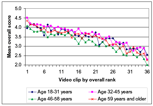
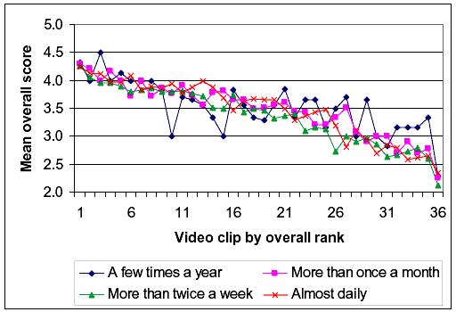
Demographic Variables An exploration of the demographic variables that we collected on the respondents showed that these variables generally had little effect on the score that the respondents provided. The next few paragraphs illustrate the general point. Figure 21 shows how respondent age affected the "overall" score they provided. The video clip rank corresponds to that provided in table 30 (i.e., clip 1 was from the White Rock Lake path and had the highest average "overall" score of the 36 clips). The plotted lines correspond to four age groups, and there were at least 20 respondents in each group. Obviously, the lines track each other very closely. The 32– to 45–year-old age group generally provided the highest scores, the 46– to 58–year–old age group generally provided the lowest scores, and the other age groups fell between those two. However, except for that shift in average score, respondents of different ages generally perceived the differences between two video clips to be about the same.
Figure 21. Effects of respondent age on overall rating
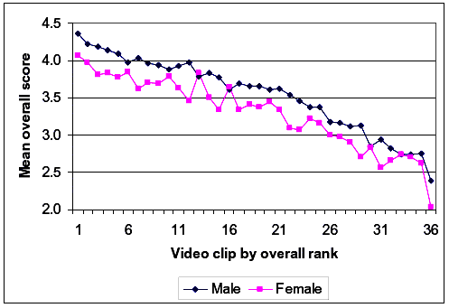
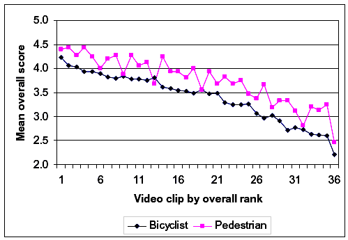
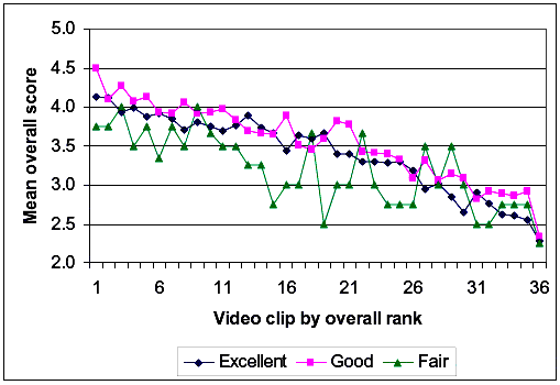
Figures 22 through 25 show lines similar to figure 21, except that the variables graphed are respondent gender, mode of travel (bicyclist versus pedestrian), health status, and trail use. Again, the pattern for all of these cases is that there were shifts from one group of respondents to another; however, respondents of different groups generally perceived the differences between two video clips to be about the same. In figure 22, we see that men generally provided higher scores than women. In figure 23, it appears that respondents from a pedestrian point of view provided generally higher scores than respondents from a bicyclist point of view. From figure 24, we note that those reporting themselves to be in fair health provided generally lower scores than those reporting themselves to be in good or excellent health. Finally, figure 25 shows no clear trend in ratings by the reported amount of trail use. Overall, these respondent demographic variables seem to matter regarding the score magnitude, but they do not seem to interact with the information on the video image of the path.
Figure 22. Effects of respondent gender on overall rating
Figure 23. Effects of path user type on overall rating.
Figure 24. Effects of respondent health status on overall rating.
Figure 25. Effects of respondent path use on overall rating
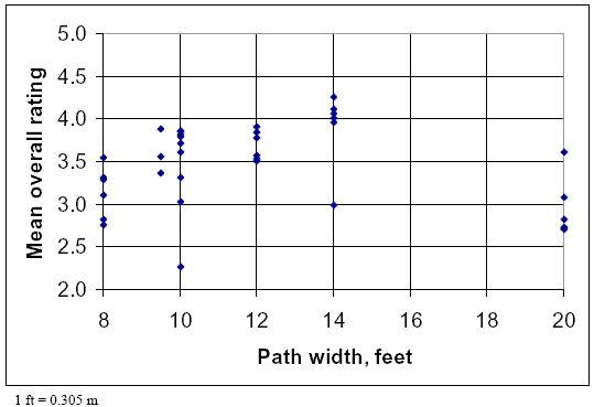
Path Design Variables A look at the relationship between path width and respondent rating shows that path width should probably be an important variable in an LOS model. Figure 26 plots path width against mean overall rating for each of the 36 video clips. The ratings appear to be generally heading upward as the path width rises from 2.4 to 4.2 m (8 to 14 ft). For the 6.1-m- (20-ft-) wide trail video clips (from the Lakefront Trail in Chicago), the average ratings fall back down; however, that may be a result of the very heavy volumes and numbers of events shown during those clips rather than the path width. A similar relationship is seen between the path width and the average rating of the lateral separation perceived by the respondents. Table 29 summarizes the responses for other key path design variables, including the presence of a centerline, the width of clear zone extending laterally from the edge of the path, and the forward sight distance along the path. The table shows average overall ratings for all of the video clips that have a particular level of a variable and average ratings for either lateral separation or the ability to pass, depending on which of those was more relevant for that variable.
Figure 26. Effects of path width on overall rating
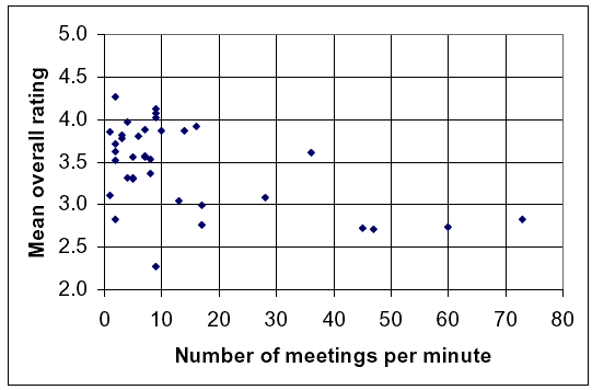
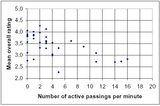
The presence of a centerline seems to be strongly related to the overall rating–paths with no centerline rated, on average, about 0.1 points better than did paths with dashed centerlines, and about 0.4 points better than did paths with solid centerlines. This may be a result of the perceived restrictions in freedom to maneuver the bicycle imposed by a centerline. Clear-zone width does not seem to have a strong or consistent relationship with average overall rating, or with the average rating of lateral separation. Finally, while paths with poor sight distances were generally rated lowest overall and for the ability to pass, improvements in sight distance above poor did not produce consistently improving ratings. Events on the Path Respondents were not in a very good position to judge the volume of traffic on the paths in the video clips since they only viewed 1-min time slices from a moving-bicyclist perspective. However, the advantage of the moving-bicyclist perspective was that we were able to convey the number of events during that minute–the meetings and passings–quite realistically. Figure 27 shows the relationship between meetings during the 1-min clip, and average overall rating, while figure 28 relates the number of active passings and the average overall rating. Both figures suggest that average ratings decline as the number of meetings and active passings rise, with the decline for active passings being a bit more pronounced. The project team had concerns for both of these graphs in the sense that the Chicago path, with its relatively large number of meetings, average overall rating, and active passings, was dominating the results from the other paths. This concern will be addressed in the next section, which describes the detailed statistical modeling of these results.
Table 29. Effects of other path design variables on average ratings.
*The path shown in these video clips had, on average, no clear zone on one side and 1.5 m (5 ft) on the other side.
Figure 27. Effects of the number of meetings on overall rating.
Figure 28. Effects of the number of active passingson overall rating.
Video Quality The final category of perception data variables that the project team analyzed was the quality of the video. As stated earlier, we chose to show the respondents videos shot from the moving-bicyclist perspective during the operational data collection in order to portray real paths with real traffic loads. However, the downside of this approach was that the quality of the video varied from quite good to quite poor. Three important qualities that captured this variability were amount of glare, quality of the focus, and amount of vertical tilt since all of these were judged by the project team. Table 30 shows how these varied in the average overall rating provided by the respondents. None of the three quality variables had a strong relationship with average overall rating. Only the glare variable appeared as if it might matter during detailed modeling efforts since the average overall rating for the video clips with no glare was higher than for video clips with some glare; however, as the amount of glare increased from low to medium to high, the average overall ratings did not continue to decline. It appears from table 30 that the respondents were able to rate the paths according to other criteria aside from video quality.
Table 30. Effects of video quality on average ratings.
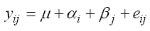
MODEL CREATIONInteractions The basic statistical model was based on a two-way layout that considered both subject characteristics and trail characteristics without interaction between the two. Below is the basic model:
where:
The interaction of subject characteristics and trail characteristics could be a potentially complicating factor in this experiment setup. The simplification brought on by excluding such an interaction has great value; moreover, the validity of the analysis would be suspect if strong interactions were present. The experiment setup precluded any replication–no subject had multiple ratings of the same video or trail under the same conditions. While the full subject-by-trail interaction could not be addressed in this model, we did look for interactions between subject characteristics and trails, and trail characteristics and subjects. In the case of subject characteristics, the appropriate model was as shown in equation 58:
where
In the case of trail characteristics, the appropriate model was as shown in equation 59:
where While the respondents were sampled from a relevant population, this sample may not be representative of some shared paths at some times, and adjustments to the model may be needed in those cases. If the characteristics of the users of a path of interest were different from those of our respondents in terms of age, gender, etc., the lack of interaction seen with these variables in trial models dictates that the effect of these changes in respondent characteristics would only make an additive shift in the ratings, and will not change the relationship with the trail characteristics. Averaging over subjects leads to the following refinement from equation 59:
where all variables are as previously defined, and the overbars and dots are reminders that we are averaging over the second subscript (respondents). The mean of the random subject effect, Choice of Overall Response Since we asked for responses for four different ratings of each video clip, we had to choose which to use in our model of quality of service of the path. We chose to create a model using the overall rating for two primary reasons. First, table 31, which provides the correlations among all the responses fit from a preliminary modeling effort using equation 48 above, shows that the responses were highly correlated among the four perception measures or responses. In fact, the overall rating was the most highly correlated with the other perception measures. Furthermore, the overall rating was designed to capture the respondents' feelings with regard to all aspects of the path scene that they were viewing; however, the other perception measures honed in on more specific aspects. For example, lateral separation will probably capture the respondents' feelings about path width, but not about the sight distance ahead on the path. For these reasons, the model development that follows is concentrated on the overall rating provided by the respondents.
Table 31. Correlation between the four perception measures.
Fitting the Model A preliminary analysis indicated that some variables appeared to be highly significant toward explaining variation in the overall rating. Careful examination, however, suggested that some variables were mere surrogates for one of the more influential, but very distinctive, trails (Lakefront in Chicago). This trail was different from the others in that it is situated in a highly urbanized environment and it was extremely crowded when we recorded the video that we showed to the respondents. Considering that most applications of this model would be outside of such an urbanized environment, the pursuit for the best model first excluded this location. Variable selection was performed with only the remaining 30 observations (instead of 36) from 9 locations. After the variables were selected, the model was then refit using all 36 observations. Thus, the responses to the Chicago path helped fit the model, but it did not have undue influence. The following trail variables were included in the variable selection process:
The variables representing trail pavement material, presence of a shoulder, and presence of a vertical curve were not considered because, for each of these variables, eight locations took one value and two locations took the other. These variables would be acting more like "dummy variables" for a single location, which would have no value in predicting the service rating for a new location. The video quality variables included in the selection process were:
The operational characteristics included in variable selection were:
Note that the factor of 10 weighting the number of active passings was constructed by fitting equation 60, not including the effect of the location characteristics. Other weightings were considered, but a weight of 10 fit best for all four response variables. A different weighting for the heavily traveled Lakefront Trail was considered and abandoned for the sake of simplicity. Because the number of potential explanatory variables exceeded the number of locations by a factor of nearly two, forward selection was employed in the model selection process. The following variables were consistently useful as explanatory variables, leading to models with high R2-values:
The investigation using 9 of the 10 locations (excluding Lakefront) led to a model that used the first 4 explanatory variables (the glare and focus variables were dropped out of the running). Including the responses to the six Lakefront video clips led to nearly the same quality of fit, and most of the coefficients were not substantially different. However, the variable for the weighted events per foot width of trail did not contribute. Dropping that variable led to a simpler model with approximately the same fit. Therefore, our recommendation as the model that best predicted the overall rating (on our 1 to 5 scale) was:
where:
Tables 32 and 33 show the analysis of variance and parameter estimate tables for this model from our statistical software (SAS). The output shows that the model fit the data well, with a high F-value that was highly significant. The R2-value for this model was a healthy 0.64, and the adjusted R2-value was also good at 0.61. The model should be easy to employ by path designers and analysts, with just three variables, two of which are under the designer's direct control and a third which is available from the methods described in chapter 3. The negative signs of the weighted events and width variables are as expected. The sign of the centerline variable is probably a result of feeling restricted by bicyclists on a path with a centerline, particularly under the relatively low-volume conditions depicted on most of the video clips. The standard error and t-values for the intercept and each of the variables showed that they were all significantly different from zero at the 95-percent level, with the weighted events and width variables being greatly different from zero. In sum, based on goodness of fit to all of the locations tested, ease of use, and logic in the relationship, equation 61 for overall rating should serve well as a quality-of-service predictor.
Table 32. Analysis of variance table for the final model.
Table 33. Parameter estimate table for the final model.
FHWA-HRT-05-137 |
|||||||||||||||||||||||||||||||||||||||||||||||||||||||||||||||||||||||||||||||||||||||||||||||||||||||||||||||||||||||||||||||||||||||||||||||||||||||||||||||||||||||||||||||||||||||||||||||||||||||||||||||||||||||||||||||||||||||||||||||||||||||||||||||||||||||||||||||||||||||||||||||||||||||||||||||||||||||||||||||||||||||||||||||||||||||||||||||||||||||||||||||||||||||||||||||||||||||||||||||||||||||||||||||||||||||||||||||||||||||||||||||||||||||||||||||||||||||||||||


 ij
ij
 i
i j
j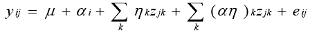
 )k. We examined the following subject characteristics–age, gender, pedestrian or bicycle point of view, and fitness level. As we suspected from the data we examined earlier in this chapter, none of these interactions proved to be sizeable.

 )k. We tested for trail pavement material, shoulder presence, shoulder width, shadow in the video, glare in the video, horizontal curvature, vertical curvature, sight distance, urban versus other environment, presence of a centerline, and average clear-zone width. The greatest interactions were found with the pavement material, presence of a shoulder, and urban versus other environment, with F-statistics in these cases as large as 4.87, 3.93, and 3.54, respectively. However, practically speaking, these were not very important interactions in a database of more than 3,500 observations. The modest size of these interaction effects, coupled with the ineffectiveness of these three variables as explanatory variables in subsequent modeling (see below), gave sufficient support for excluding these interactions from the model.


