Bridges & Structures

<< Previous

Contents

Next >>

Geotechnical Aspects of Pavements Reference Manual

Chapter 3.0 Geotechnical Issues In Pavement Design And Performance (continued)

3.5 Incorporation Of Geotechnical Factors In Pavement Design

3.5.1 Pavement Design Methodologies

The terms empirical design, mechanistic design, and mechanistic-empirical design are frequently used to identify general approaches toward pavement design. The key features of these design methodologies are described in the following subsections.

Empirical Design

An empirical design approach is one that is based solely on the results of experiments or experience. Observations are used to establish correlations between the inputs and the outcomes of a process - e.g., pavement design and performance. These relationships generally do not have a firm scientific basis, although they must meet the tests of engineering reasonableness (e.g., trends in the correct directions, correct behavior for limiting cases, etc.). Empirical approaches are often used as an expedient when it is too difficult to define theoretically the precise cause-and-effect relationships of a phenomenon.

The principal advantages of empirical design approaches are that they are usually simple to apply and are based on actual real-world data. Their principal disadvantage is that the validity of the empirical relationships is limited to the conditions in the underlying data from which they were inferred. New materials, construction procedures, and changed traffic characteristics cannot be readily incorporated into empirical design procedures.

Mechanistic Design

The mechanistic design approach represents the other end of the spectrum from the empirical methods. The mechanistic design approach is based on the theories of mechanics to relate pavement structural behavior and performance to traffic loading and environmental influences. The mechanistic approach for rigid pavements has its origins in Westergaard's development during the 1920s of the slab on subgrade and thermal curling theories to compute critical stresses and deflections in a PCC slab. The mechanistic approach for flexible pavements has its roots in Burmister's development during the 1940s of multilayer elastic theory to compute stresses, strains, and deflections in pavement structures.

A key element of the mechanistic design approach is the accurate prediction of the response of the pavement materials - and, thus, of the pavement itself. The elasticity-based solutions by Boussinesq, Burmister, and Westergaard were an important first step toward a theoretical description of the pavement response under load. However, the linearly elastic material behavior assumption underlying these solutions means that they will be unable to predict the nonlinear and inelastic cracking, permanent deformation, and other distresses of interest in pavement systems. This requires far more sophisticated material models and analytical tools. Much progress has been made in recent years on isolated pieces of the mechanistic performance prediction problem. The Strategic Highway Research Program during the early 1990s made an ambitious but, ultimately, unsuccessful attempt at a fully mechanistic performance system for flexible pavements. To be fair, the problem is extremely complex; nonetheless, the reality is that a fully mechanistic design approach for pavement design does not yet exist. Some empirical information and relationships are still required to relate theory to the real world of pavement performance.

Mechanistic-Empirical Design Approach

As its name suggests, a mechanistic-empirical approach to pavement design combines features from both the mechanistic and empirical approaches. The mechanistic component is a mechanics-based determination of pavement responses, such as stresses, strains, and deflections due to loading and environmental influences. These responses are then related to the performance of the pavement via empirical distress models. For example, a linearly elastic mechanics model can be used to compute the tensile strains at the bottom of the asphalt layer due to an applied load; this strain is then related empirically to the accumulation of fatigue cracking distress. In other words, an empirical relationship links the mechanistic response of the pavement to its expected or observed performance.

The development of mechanistic-empirical design approaches dates back at least four decades. Huang (1993) notes that Kerkhoven and Dormon (1953) were the first to use the vertical compressive strain on top of the subgrade as a failure criterion for permanent deformation in flexible pavement systems, while Saal and Pell (1960) recommended the use of horizontal tensile strain at the bottom of the AC layer to minimize fatigue cracking. Likewise, Barenberg and Thompson (1990) note that mechanistic-based design procedures for concrete pavements have also been pursued for many years. Several design methodologies based on mechanistic-empirical concepts have been proposed over the years, including the Asphalt Institute procedure (Shook et al., 1982) for flexible pavements, the PCA procedure for rigid pavements (PCA, 1984), the AASHTO 1998 Supplemental Guide (AASHTO, 1998) for rigid pavements, and the NCHRP 1-26 procedures (Barenberg and Thompson, 1990, 1992) for both flexible and rigid pavements. Some mechanistic-empirical design procedures have also been implemented at the state level (e.g., Illinois, Kentucky, Washington, and Minnesota; see also Newcomb and Birgisson, 1999).

3.5.2 The AASHTO Pavement Design Guides

The AASHTO Guide for Design of Pavement Structures is the primary document used to design new and rehabilitated highway pavements. The Federal Highway Administration's 1995-1997 National Pavement Design Review found that some 80 percent of states use the 1972, 1986, or 1993 AASHTO Guides² (AASHTO, 1972; 1986; 1993). Of the 35 states that responded to a 1999 survey by Newcomb and Birgisson (1999), 65% reported using the 1993 AASHTO Guide for both flexible and rigid pavement designs.

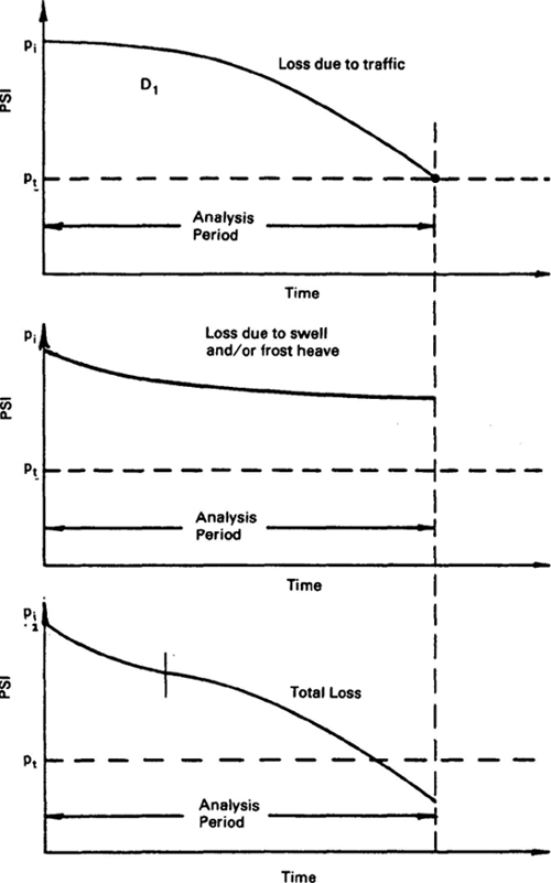
All versions of the AASHTO Design Guide are empirical methods based on field performance data measured at the AASHO Road Test in 1958-60, with some theoretical support for layer coefficients and drainage factors. The overall serviceability of a pavement during the original AASHO Road Test was quantified by the Present Serviceability Rating (PSR; range = 0 to 5), as determined by a panel of highway raters. This qualitative PSR was subsequently correlated with more objective measures of pavement condition (e.g., cracking, patching, and rut depth statistics for flexible pavements) and called the Pavement Serviceability Index (PSI). Pavement performance was represented by the serviceability history of a given pavement - i.e., by the deterioration of PSI over the life of the pavement (Figure 3-8). Roughness is the dominant factor in PSI and is, therefore, the principal component of performance under this measure.

Figure 3-8. Pavement serviceability in the AASHTO Design Guides (AASHTO, 1993).

Each successive version of the AASHTO Design Guide has introduced more and more sophisticated geotechnical concepts into the pavement design process. The 1986 Guide in particular introduced important refinements for materials input parameters, design reliability, and drainage factors, as well as empirical procedures for rehabilitation design. Enhancements were made to both the flexible and rigid design methodologies, although the impact is perhaps more significant for flexible pavements because of the greater contribution of the unbound layers to the structural capacity of these systems. The evolution of geotechnical considerations in the various versions of the AASHTO Design Guides is highlighted in the following sections.

1961 Interim Guide

The 1961 Interim AASHO Pavement Design Guide contained the original empirical equations relating traffic, pavement performance, and structure, as derived from the data measured at the AASHO Road Test (HRB, 1962). These equations were specific to the particular foundation soils, pavement materials, and environmental conditions at the test site in Ottawa, Illinois. The empirical equation for the flexible pavements at the AASHO Road Test is:

(3.1)

logW18 = 9.36 log( SN + 1 ) - 0.20 +	log[ ( 4.2 - pt ) / ( 4.2 - 1.5 ) ]
	0.4 + 1094 / ( SN + 1 )5.19

in which

W18	=	number of 18 kip equivalent single axle loads (ESALs)
pt	=	terminal serviceability at end of design life
SN	=	structural number

Equation (3.1) must be solved implicitly for the structural number SN as a function of the other input parameters. The structural number SN is defined as:

(3.2)

SN = a₁D₁ + a₂D₂ + a₃D₃

in which D₁, D₂, and D₃ are the thicknesses (inches) of the surface, base, and subbase layers, respectively, and a₁, a₂, and a₃ are the corresponding layer coefficients. For the materials used in the majority of the flexible pavement sections at the AASHO Road Test, the values for the layer coefficients were determined as a₁=0.44, a₂=0.14, and a₃=0.11. Note that there may be many combinations of layer thicknesses that can provide satisfactory SN values; cost and other issues must be considered as well to determine the final design layer structure.

The corresponding empirical design equation relating traffic, performance, and structure for the rigid pavements at the AASHO Road Test is:

(3.3)

logW18 = 7.35 log( D + 1 ) - 0.06 +	log[ ( 4.5 - pt) / ( 4.5 - 1.5 ) ]
	1 + 1.624 × 107 / ( D + 1 )8.46

in which D is the pavement slab thickness (inches) and the other terms are as defined previously. Equation (3.3) must be solved implicitly for the slab thickness D as a function of the other input parameters.

Since Eqs. (3.1) through (3.3) are for the specific foundation soils, materials, and environmental conditions at the AASHO Road Test site, there are no geotechnical or environmental inputs to determine. This clearly limited the applicability of these design equations to other sites and other conditions and was the primary motivation behind the development of the 1972 Interim Guide.

1972 Interim Guide

The 1972 Interim Design Guide (AASHTO, 1972) was the first attempt to extend the findings from the AASHO Road Test to foundation, material, and environmental conditions different from those at the test site. This was done through the introduction of several new features for the flexible and rigid pavement design. A rudimentary overlay design procedure was also included in the 1972 Interim Guide.

Flexible Pavements

The major new features added to the 1972 Interim Guide to extend its flexible pavement design methodology to conditions other than those at the AASHO Road Test were:

• An empirical soil support scale to reflect the influence of local foundation soil conditions in Equation (3.1). This soil support scale ranged from 1 to 10, with a soil support value S_i of 3 corresponding to the silty clay foundation soils at the AASHO Road Test site and the upper value of 10 corresponding to crushed rock base materials. All other points on the scale were assumed from experience, with some limited checking through theoretical computations. It is important to note that "the units of soil support, represented by the soil support scale, have no direct relationship to any procedure for testing soils" (AASHTO, 1972) and that it was left up to each agency to determine correlations between soil support and material testing procedures.
• An empirical regional factor R to provide an adjustment to the structural number SN in Equation (3.2) for local environmental and other considerations. Values for the regional factor were estimated from serviceability reduction rates in the AASHO Road Test. These estimates varied between 0.1 and 4.8, with an annual average value of about 1.0. Recommended values for the regional factor based on the AASHO Road Test results are summarized in Table 3-3. However, the Guide cautions that "the regional factor may not adjust for special conditions, such as serious frost conditions, or other local problems" and that "considerable judgment must still be exercised in evaluating [environmental] effects and in selecting an appropriate regional factor for design" (AASHTO, 1972).

  Table 3-3. Recommended values for Regional Factor R (AASHTO, 1972).

  Roadbed Material Condition	R
  Frozen to depth of 5" (130 mm) or more (winter)	0.2 to 1.0
  Dry (summer and fall)	0.3 to 1.5
  Wet (spring thaw)	4.0 to 5.0

• Guidelines for estimating structural layer coefficients a₁, a₂, and a₃ in Equation (3.2) for materials other than those at the AASHO Road Test. These guidelines were based primarily on a survey of state highway agencies regarding the values for the layer coefficients that they were currently using in design for various materials. Ranges of layer coefficient values reported in this survey are summarized in Table 3-4. The Guide recommends that "Because of widely varying environments, traffic, and construction practices, it is suggested that each design agency establish layer coefficients applicable to its own experience. Careful consideration should be given before adoption of values developed by others" (AASHTO, 1972).

  Table 3-4. Ranges of structural layer coefficients from agency survey (AASHTO, 1972).

  Coefficient	Low Value	High Value
  a1 (surface)	0.17	0.45
  a2 (untreated base)	0.05	0.18
  a3 (subbase)	0.05	0.14

The modified version of Equation (3.1) for flexible pavements implemented in the 1972 Interim Guide is as follows:

(3.4)

logW18 = 9.36 log( SN + 1 ) - 0.20 + log[ ( 4.2 - pt ) / ( 4.2 - 1.5 ) ]   0.40 + 1094 / ( SN + 1 )5.19

+ log 1 + 0.372 ( Si - 3.0 )   R

in which R is the regional factor, S_i is the soil support value, and the other terms are as defined previously. As in the 1961 Interim Guide, the thicknesses for each pavement layer are determined as functions of the structural layer coefficients using Equation (3.2) and the required SN determined from Equation (3.4). The principal geotechnical inputs in the design procedure are thus the soil support value S_i for the subgrade and the structural layer coefficients a₂, a₃ and thicknesses D₂, D₃ for the base and subbase layers, respectively.

Rigid Pavements

Only one major new feature was added to the 1972 Interim Guide to extend its rigid pavement design methodology to conditions other than those at the AASHO Road Test. This was the use of the Spangler/Westergaard theory for stress distributions in rigid slabs to incorporate the effects of local foundation soil conditions. The foundation soil conditions are characterized by the overall modulus of subgrade reaction k, which is a measure of the stiffness of the foundation soil.³

Interestingly, the modifications made to the rigid pavement design procedure in the 1972 Interim Guide do not include a regional factor for local environmental conditions similar to that implemented in the flexible design procedure. The explanation offered for this was that "it was not possible to measure the effect of variations in climate conditions over the two-year life of the pavement at the Road Test site" (AASHTO, 1972).

The modified version of Equation (3.3) for rigid pavements implemented in the 1972 Interim Guide is as follows:

(3.5)

logW18 = 7.3 log( D + 1 ) - 0.06 + log[ ( 4.5 - pt ) / ( 4.5 - 1.5 ) ]   1 + 1.624 × 107 / ( D + 1 )8.46

+ ( 4.22 - 0.32 pt )   log   Sc     D0.75 - 1.132         215.63 J D0.75 - 18.42 / ( Ec / k )0.25

in which S_c is the modulus of rupture and E_c is the modulus of elasticity for the concrete (psi), J is an empirical joint load transfer coefficient, k is the modulus of subgrade reaction (pci), and all other terms are as defined previously. Note that k, the principle geotechnical input in the 1972 rigid pavement design procedure, is a "gross" k defined as load (stress) divided by deflection, and as such it includes both elastic and inelastic response of the foundation soil.

For the design of reinforcement in jointed reinforced concrete pavements (JRCP), one additional geotechnical design input is required: the friction coefficient between the slab and the subbase/subgrade.

Sensitivity to Geotechnical Inputs

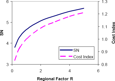
The sensitivity of the pavement design to the new geotechnical properties in the 1972 AASHTO Guide can be illustrated via some simple examples. Figure 3-9 shows the variation of the required structural number SN with the soil support factor S_i for a three-layer (asphalt, base, subgrade) flexible pavement system with design traffic W₁₈ = 10 million, regional factor R = 1 (i.e., the environmental conditions at the AASHO Road Test), and terminal serviceability p_t = 2.5. Also shown in the figure is the pavement cost index as a function of soil support, assuming that asphalt is twice as expensive per inch of thickness than crushed stone base and that the cost index equals 1 at S_i = 3 (i.e., the foundation conditions in the AASHO Road Test). Figure 3-10 shows similar variations of SN and cost index with the regional factor R for the same three-layer flexible pavement and S_i = 3. The results for this example suggest that the pavement design and cost is quite sensitive to soil support (cost index varying between 0.3 and 1.3 over the range of valid S_i values), but only moderately sensitive to the regional factor (cost index varying by about ± 20% over the range of valid R values).

Figure 3-9. Sensitivity of 1972 AASHTO flexible pavement design to foundation support quality.

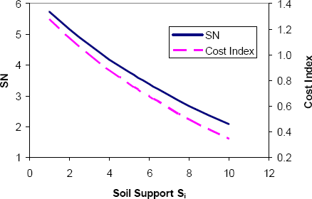
Figure 3-10. Sensitivity of 1972 AASHTO flexible pavement design to environmental conditions.

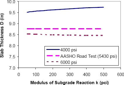
The sensitivity of rigid pavement slab thickness to the modulus of subgrade reaction k is summarized in Figure 3-11 for three different concrete compressive strength values. The results confirm the conventional wisdom that rigid pavement designs are relatively insensitive to foundation stiffness.

Figure 3-11. Sensitivity of 1972 AASHTO rigid pavement design to foundation stiffness (1 in = 25 mm; 1 pci = 284 MN/m³).

1986 Guide

The 1986 AASHTO Design Guide (AASHTO, 1986) retained the basic approach from the 1972 Interim Guide but added several new features. Key among these are a more rational characterization of subgrade and unbound materials in terms of the resilient modulus, the explicit consideration of the benefits of pavement drainage (and conversely the consequences of poor drainage), and better treatment of environmental influences on pavement performance. Additional significant enhancements in the 1986 Guide include the incorporation of a reliability factor into the design, expanded treatment of rehabilitation (both with and without overlays), and life-cycle cost analysis.

The geotechnical-related enhancements in the 1986 Guide include the following:

Flexible and Rigid Pavements

• Use of the resilient modulus M_R (AASHTO T272) as a stiffness parameter for characterizing the soil support provided by the subgrade. The resilient modulus M_R is a measure of the elastic stiffness of the soil recognizing certain nonlinear characteristics. It is a basic material property that can be measured directly using established laboratory test protocols, evaluated in-situ from nondestructive tests, or estimated using various empirical relations as detailed later in Chapter 5.
• Improvements in incorporating the effects of environment on pavement performance. Specific emphasis is given to frost heave, thaw-weakening, and swelling of subgrade soils. The enhancements in the 1986 Guide for environmental effects include
  • The explicit separation of total serviceability loss ΔPSI into load- and environment-related components: (3.6)

    ΔPSI = ΔPSI_TR + ΔPSI_SW + ΔPSI_FH

    in which ΔPSI_TR, ΔPSI_SW and ΔPSI_FH are the components of serviceability loss attributable to traffic, swelling, and frost heave, respectively.

  • Estimation of an effective resilient modulus for the roadbed that reflects the seasonal variations in subgrade stiffness.
• Incorporation of reliability considerations to reflect the inevitable uncertainty and variability in the design inputs and the importance of the project. Reliability is incorporated in the design through factors that increase the design traffic level.

Flexible Pavements

The geotechnical-related enhancements to the flexible pavement design procedures in the 1986 AASHTO Guide included the following:

• Use of the resilient modulus for determining the structural layer coefficients for both stabilized and unstabilized unbound materials in flexible pavements. The structural layer coefficients a₂ and a₃ for base and subbase materials are estimated via correlations with resilient modulus; these regressions are detailed later in Chapter 5, Section 5.4.5. Nomographs that relate layer coefficients for unstabilized and stabilized base and subbase materials to other strength and stiffness properties are also provided in the 1993 Guide. It is important to remember, however, that these relations for the structural layer coefficients are largely empirical and are based primarily on engineering judgment with only limited amounts of data.
• Guidance for the design of subsurface drainage systems and modifications to the flexible pavement design equations to take advantage of improvements in performance due to good drainage. The benefits of drainage are incorporated into the structural number via empirical drainage coefficients: (3.7)

  SN = a₁D₁ + a₂D₂m₂ + a₃D₃m₃

  in which m₂ and m₃ are the drainage coefficients for the base and subbase layers, respectively, and all other terms are as defined previously. The empirical values for m_i, which are specified in terms of quality of drainage and the estimated percentage of time the layer will be near saturation, range from 0.4 to 1.4. Section 5.5.1 in Chapter 5 provides the details for estimating the m_i input values for design. The development of these values can be found in Appendix DD of the 1986 AASHTO Guide.

  The modified version of Equation (3.4) for flexible pavements implemented in the 1986 Guide is as follows:

  (3.8)

  log₁₀(W₁₈) = Z_RS₀ + 9.36 log₁₀( SN + 1 ) - 0.20

  +	log10		ΔPSI		+ 2.32 log10( MR ) - 8.07
  			4.2 - 1.5
  	0.40 +		1094
  			( SN + 1 )5.19

  in which Z_R is a function of the design reliability level, S₀ is a measure of the overall uncertainty or variability of the design inputs and performance prediction, M_R is the subgrade resilient modulus, and the other terms are as defined previously. Equation (3.7) is used to determine the layer thicknesses required to achieve the total SN value required by Equation (3.8).

In summary, the explicit geotechnical inputs in the 1986 flexible design procedure are the:

• seasonally adjusted subgrade resilient modulus M_R,
• base and subbase resilient moduli E_BS and E_SB (used to determine the a₂ and a₃ structural layer coefficients),
• base and subbase drainage coefficients m₂ and m₃, and
• base and subbase layer thicknesses D₂ and D₃.

Rigid Pavements

The geotechnical-related enhancements to the rigid pavement design procedures in the 1986 AASHTO Guide included the following:

• Guidance for the design of subsurface drainage systems and modifications to the rigid pavement design procedure to take advantage of improvements in performance due to good drainage. The benefits of drainage are incorporated in the rigid pavement design equation via an empirical drainage coefficient C_d. The empirical values for C_d, which are specified in terms of quality of drainage and the estimated percentage of time the pavement will be near saturation, range from 0.7 to 1.25. Section 5.5.1 in Chapter 5 provides the details for estimating the C_d input values for design.
• Enhancements to the procedures for estimating a composite modulus of subgrade reaction that explicitly incorporate the influence of subbase type and thickness, the presence of shallow bedrock, and seasonal variations in subgrade and subbase resilient moduli.
• Adjustment of the design equations to account for the potential loss of support arising from subbase erosion and/or differential vertical soil movements. A loss of support factor LS is used to determine the effective k value for the foundation soil. Section 5.4.6 in Chapter 5 summarizes the recommended values for LS in the 1986 AASHTO Guide for various subbase material types.

The modified version of Equation (3.5) for rigid pavements implemented in the 1986 Guide is as follows:

(3.9)

log₁₀( W₁₈ ) = Z_RS₀ + 7.35 log₁₀( D + 1 ) - 0.06

+

log10

ΔPSI

+ ( 4.22 - 0.32 pt ) log10

Sc Cd ( D0.75 - 1.132 )

4.5 - 1.5

1 +

1.64 × 107

215.63 J

D0.75 -

18.42

( D + 1 )8.46

( Ec / k )0.25

in which C_d is the drainage coefficient and the other terms are as defined previously.

In summary, the explicit geotechnical inputs in the 1986 rigid pavement design procedure are:

• The seasonally adjusted effective modulus of subgrade reaction k. This in turn is a function of the seasonally adjusted values for the subgrade and subbase resilient moduli M_R and E_SB, the thickness of the subbase D_SB, the subgrade depth to rigid foundation D_SG, and the loss of support factor LS.
• The drainage coefficient C_d.
• A friction factor related to the frictional resistance between the slab and subbase/subgrade for reinforcement design in JRCP pavements.

Sensitivity to Geotechnical Inputs

The key geotechnical inputs in the 1986 AASHTO design procedure for flexible pavements are:

• foundation stiffness, as characterized by the subgrade resilient modulus (M_R), and
• moisture and drainage, as characterized by the layer drainage coefficients (m_i).

For rigid pavements, the key geotechnical inputs are:

• foundation stiffness, as characterized by the resilient moduli of the subgrade (M_R) and granular subbase (E_SB) and the thickness of the subbase (D_SB).
• erodibility of the granular subbase, as characterized by the Loss of Support factor (LS).
• moisture and drainage, as characterized by the drainage coefficient (C_d).

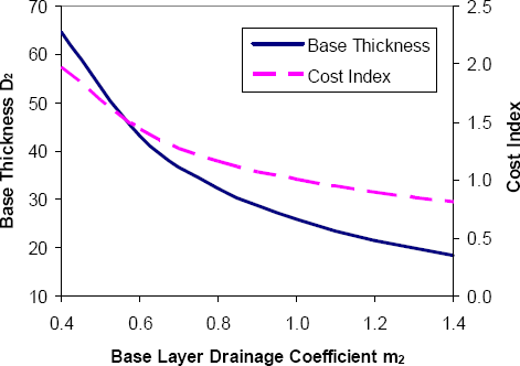
The sensitivity of the pavement design to the geotechnical inputs in the 1986 AASHTO Guide can be illustrated via some simple examples. Table 3-5 summarizes assumed baseline design inputs for a typical flexible pavement section. These values (except for traffic) generally conform to those at the AASHO Road Test. The variation of required pavement structure with subgrade stiffness and drainage for these conditions are summarized in Figure 3-12 and Figure 3-13, respectively. Also shown in these figures is a pavement cost index, which is based on the assumption that asphalt concrete is twice as expensive as crushed stone base per inch of thickness; the cost index is normalized to 1.0 at baseline conditions (i.e., values in Table 3-5). The vertical cost axes in Figure 3-12 and Figure 3-13 have been kept constant in order to highlight the relative sensitivities of cost to subgrade stiffness and drainage conditions. The horizontal axes in the figures span the full range of stiffness and drainage conditions for flexible pavements.

Table 3-5. Flexible pavement baseline conditions for 1986 AASHTO sensitivity study.

Input Parameter	Design Value
Traffic (W18)	10 × 106 ESALs
Reliability	90%
Reliability factor (ZR)	-1.282
Overall standard error (So)	0.45
Allowable serviceability deterioration (ΔPSI)	1.7
Subgrade resilient modulus (MR)	3,000 psi (20.7 MPa)
Granular base resilient modulus (EBS)	30,000 psi (207 MPa)
Granular base layer coefficient (a2)	0.14
Granular base drainage coefficient (m2)	1.0
Asphalt concrete layer coefficient (a1)	0.44

Figure 3-12. Sensitivity of 1986 AASHTO flexible pavement design to subgrade stiffness (1 psi = 6.9 kPa).

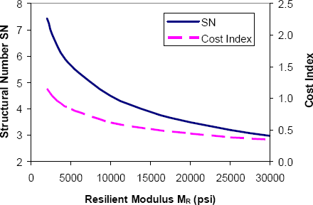
Figure 3-13. Sensitivity of 1986 AASHTO flexible pavement design to drainage conditions (1 inch = 25 mm).

Both the structural number and pavement cost are highly sensitive to foundation stiffness. As shown in Figure 3-12, reducing M_R from 20,000 psi (138 MPa, corresponding to a CBR of about 30) to 2000 psi (13.8 MPa, corresponding to a CBR value of about 2) results in a 115% increase in required total structural number. This translates to a corresponding 170% increase in cost.

From Equation (3.8), it is clear that changing the drainage coefficient m₂ for the base layer will not affect the total required structural number SN (nor will it directly affect the required structural number for each of the layers). However, changes in drainage do directly affect the structural effectiveness of the granular material in the base layer and, thus, its thickness and cost. As shown in Figure 3-13, reducing m₂ from its maximum value of 1.4 to its minimum value of 0.4 requires more than a 3-fold increase in required base thickness. This translates to a 150% increase in overall pavement structural cost for these example conditions.

A similar sensitivity analysis can be performed for the rigid pavement design procedure in the 1986 AASHTO Guide. Table 3-6 summarizes assumed design inputs for a typical rigid pavement section. Again, these values (except for traffic) generally conform to those at the AASHO Road Test. The variations of required slab thickness with foundation stiffness, base erodibility, and drainage conditions are summarized in Figure 3-14, Figure 3-15, and Figure 3-16, respectively. The vertical axes in Figure 3-14 through Figure 3-16 have been kept constant in order to highlight the relative sensitivities of slab thickness to the respective geotechnical inputs. Since rigid pavement cost essentially varies directly with slab thickness, a cost index is not included in the figures. The horizontal axes in the figures span the full range of stiffness, erodibility, and drainage conditions for rigid pavements.

Table 3-6. Rigid pavement baseline conditions for 1986 AASHTO sensitivity study.

Input Parameter	Design Value
Traffic (W18)	10 × 106 ESALs
Reliability	90%
Reliability factor (ZR)	-1.282
Overall standard error (So)	0.35
Allowable serviceability deterioration (ΔPSI)	1.9
Terminal serviceability level (pt)	2.5
Subgrade resilient modulus (MR)	3,000 psi (20.7 MPa)
Granular subbase resilient modulus (EBS)	30,000 psi (207 MPa)
Granular subbase resilient modulus (ESB)	30,000 psi (207 MPa)
Drainage coefficient (Cd)	1.0
Loss of Support (LS)	1.0
PCC modulus of rupture (Sc′)	690 psi (4.8 MPa)
PCC modulus of elasticity (Ec)	4.2 × 106 psi (29 GPa)
Joint load transfer coefficient (J)	4.1

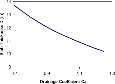
Figure 3-14 clearly shows that slab thickness is quite insensitive to foundation stiffness. This conforms to conventional wisdom, and in fact is one of the reasons that rigid pavements are often considered when foundation soils are very poor. Erodibility of the granular subbase is somewhat more important. As shown in Figure 3-15, increasing LS from 0 (least erodible) to 3 (most erodible) results in an additional 1.0 inch (25 mm) of required slab thickness. By far the most important rigid pavement geotechnical input is the moisture/drainage condition. As shown in Figure 3-16, decreasing the drainage coefficient C_d from its maximum value of 1.25 to its minimum value of 0.7 results in a 3.5 inch (87.5 mm) or 35% increase in required slab thickness for these example conditions.

Figure 3-14. Sensitivity of 1986 AASHTO rigid pavement design to subgrade stiffness (1 inch = 25 mm; 1 psi = 6.9 kPa; 1 pci = 284 MN/m³).

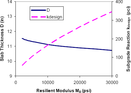
Figure 3-15. Sensitivity of 1986 AASHTO rigid pavement design to subbase erodibility (1 inch = 25 mm; 1 pci = 284 MN/m³).

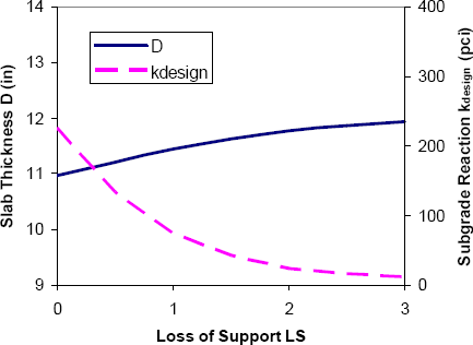
Figure 3-16. Sensitivity of 1986 AASHTO rigid pavement design to drainage conditions (1 inch = 25 mm).

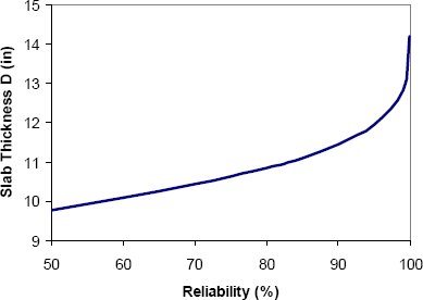
Another of the new parameters introduced in the 1986 Design Guide is design reliability. The target reliability level is set by agency policy; Table 3-7 summarizes common recommendations for design reliability for different road categories. Although reliability is not strictly a geotechnical parameter, it is useful to examine the sensitivity of pavement designs to the target reliability level. Figure 3-17 and Figure 3-18 summarize the sensitivity of the example flexible and rigid pavement designs (design inputs in Tables 3-5 and 3-6) to the design reliability level. It is clear from these figures that the required pavement structure is quite sensitive to the design reliability level, especially for the higher reliability levels. Increasing the design reliability level from 50% to 99.9% increases both the required SN and cost for flexible pavements by approximately 50% for these example conditions. The increase in required slab thickness for rigid pavements is of a similar magnitude. These increases in design structure in essence correspond to a safety factor based on agency policy for the design reliability level.

Table 3-7. Suggested levels of reliability for various functional classifications (AASHTO 1986).

Functional classification	Recommended level of reliability (%)
	Urban	Rural
Interstate and other freeways	85-99.9	80-99.9
Principal arterials	80-99	75-95
Collectors	80-95	75-95
Local	50-80	50-80

Note: Results based on a survey of AASHTO Pavement Design Task Force.

Figure 3-17. Sensitivity of 1986 AASHTO flexible pavement design to reliability level.

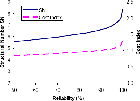
Figure 3-18. Sensitivity of 1986 AASHTO rigid pavement design to reliability level (1 inch = 25 mm).

1993 Guide

The major additions to the 1993 version of the AASHTO Pavement Design Guide (AASHTO, 1993) were in the areas of rehabilitation designs for flexible and rigid pavement systems using overlays. The only significant change to the geotechnical aspects of pavement design was the increased emphasis on nondestructive deflection testing for evaluation of the existing pavement and backcalculation of layer moduli. All other geotechnical aspects are identical to those in the 1986 Guide.

A summary of the design procedures for flexible and rigid pavements in the 1993 AASHTO Guide is provided in Appendix C. A detailed discussion of the key geotechnical inputs in the 1993 AASHTO Guide is presented in Chapter 5. Examples of the sensitivity of the pavement structural design to the various geotechnical factors included in the 1993 AASHTO Guide are the focus of Chapter 6.

1998 Guide Supplement

The 1998 supplement to the 1993 AASHTO Pavement Design Guide (AASHTO, 1998) provided an alternate method for rigid pavement design. The main changes from the procedures in the 1993 Guide included the following:

• The modulus of subgrade reaction k is now defined as the elastic value on the top of the subgrade (or embankment, if present). When measured in a plate loading test, only the elastic (i.e., recoverable) deformation is now used to compute k, and all permanent deformation is neglected. This is in contrast to previous versions of the Guide which defined k as a gross value that included both the elastic and permanent deformations from plate loading tests. Recommended procedures in the 1998 Guide Supplement for determining k are (a) correlations with soil type and other soil properties or tests; (b) deflection testing and backcalculation (most highly recommended); and (c) plate bearing tests.
• The design k value is still modified for the influence of shallow bedrock, as in the 1993 Guide. A new modification is also included for the effects of embankments.
• The effective k value for design is no longer modified for the stiffness and thickness of the base⁴ layer, as in the 1993 Guide. Instead, the base layer thickness and resilient modulus are included explicitly in the revised rigid pavement design equations.
• The drainage factor C_d is no longer included in the design equations.
• The loss of support factor LS is no longer included in the design procedure.
• Both load and temperature stresses are included in the design calculations.

A set of revised design equations for the alternate rigid pavement design method are provided in the 1998 supplement. The principal geotechnical parameters in these equations are: effective elastic modulus of subgrade support (k); modulus of elasticity of the base (E_b); and thickness of the base layer (H_b). The coefficient of friction between the slab and the base/subgrade is also required for reinforcement design in JRCP systems.

3.5.3 The NCHRP 1-37A Pavement Design Guide⁵

The various editions of the AASHTO Guide for Design of Pavement Structures have served well for several decades. These procedures are all based on performance data from the original AASHO Road Test (HRB, 1962). However, the range of conditions considered in the AASHO Road Test were quite limited, and these increasingly serious deficiencies limit the continued use of the AASHTO Design Guide as the nation's primary pavement design procedure:

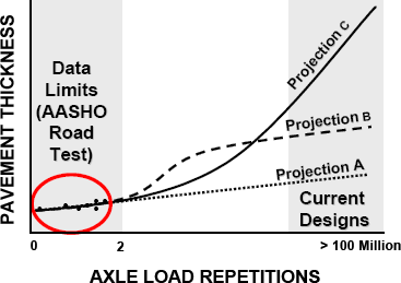
• Traffic loading: Heavy truck traffic levels have increased tremendously. The original Interstate pavements were designed in the 1960s for 5 - 10 million equivalent single-axle loads, whereas today these same pavements must be designed for 50 - 200 million axle loads, and sometimes more. It is unrealistic to expect that the existing AASHTO Guide based on the data from the original AASHO Road Test can be used reliably to design for this level of traffic. The pavements in the AASHO Road Test sustained slightly over 1 million axle load applications-less than the traffic carried by many modern pavements within the first few years of their use. When applying these procedures to modern traffic streams, the designer must extrapolate the design methodology far beyond the original field data (Figure 3-19). Such highly-trafficked projects are likely either under-designed or over-designed to an unknown degree, with significant economic inefficiency in either case.

  Figure 3-19. Extrapolation of traffic levels in current AASHTO pavement design procedures (NHI Course 131064).

  

• Rehabilitation limitations: Pavement rehabilitation design procedures were not considered at the AASHO Road Test. The rehabilitation design recommendations in the 1993 Guide are completely empirical and very limited, especially under heavy traffic conditions. Improved capabilities for rehabilitation design are vital to today's highway designs, as most projects today involve rehabilitation rather than new construction.
• Climatic conditions: Because the AASHO Road Test was conducted at one geographic location, the effects of different climatic conditions can only be included in a very approximate manner in the AASHTO Design Guides. A significant amount of distress at the original AASHO Road Test occurred in the pavements during the spring thaw, a condition that does not exist in a large portion of the country. Direct consideration of site-specific climatic effects will lead to improved pavement performance and reliability.
• Subgrade types: One type of subgrade-and a poor one at that (AASHTO A-6/A-7-6)-existed at the Road Test, but many other types exist nationally. The significant influence of subgrade support on the performance of highway pavements can only be included very approximately in the current AASHTO design procedures.
• Surfacing materials: Only a single asphalt concrete and Portland cement concrete mixture were used at the Road Test. The HMAC and PCC mixtures in common use today (e.g., Superpave, stone-mastic asphalt, high-strength PCC) are significantly different and better than those at the Road Test, but the benefits from these improved materials cannot be fully considered in the existing AASHTO Guide procedures.
• Base materials: Only two unbound dense granular base/subbase materials were included in the main flexible and rigid pavement sections of the AASHO Road Test (limited testing of stabilized bases was included for flexible pavements). These exhibited significant loss of modulus due to frost and erosion. Today, various stabilized types are used routinely, especially for heavier traffic loadings.
• Traffic: Truck suspension, axle configurations, and tire types and pressures were representative of the types used in the late 1950s. Many of these are outmoded (tire pressures of 80 psi versus 115 psi today), and pavement design procedures based on the older, lower tire pressures may be deficient for today's higher values.
• Construction and drainage: Pavement designs, materials, and construction were representative of those used at the time of the Road Test. No subdrainage was included in the Road Test sections, but positive subdrainage has become common in today's highways.
• Design life: Because of the short duration of the Road Test, the long-term effects of climate and aging of materials were not addressed. The AASHO Road Test was conducted over 2 years, while the design lives for many of today's pavements are 20 to 50 years. Direct consideration of the cyclic effect on materials response and aging are necessary to improve design life reliability.
• Performance deficiencies: Earlier AASHTO procedures relate the thickness of the pavement surface layers (asphalt layers or concrete slab) to serviceability. However, research and observations have shown that many pavements need rehabilitation for reasons that are not related directly to pavement thickness (e.g., rutting, thermal cracking, faulting). These failure modes are not considered directly in the current AASHTO Guide.
• Reliability: The 1986 AASHTO Guide included a procedure for considering design reliability that has never been fully validated. The reliability multiplier for design traffic increases rapidly with reliability level and may result in excessive layer thicknesses for heavily trafficked pavements that may not be warranted.

The latest step forward in mechanistic-empirical design is the recently-completed NCHRP Project 1-37A Development of the 2002 Guide for the Design of New and Rehabilitated Pavement Structures (NCHRP, 2004). NCHRP Project 1-37A was a multi-year effort to develop a new national pavement design guide based on mechanistic-empirical principles. A key distinction of the models developed under NCHRP Project 1-37A is their calibration and validation using data from the FHWA Long Term Pavement Performance Program national database in a well-balanced experiment design representing all regions of the country. The NCHRP 1-37A models also include flexibility for re-calibration and validation using local or regional databases, if desired, by individual agencies. The mechanistic-empirical design approach as implemented in the NCHRP 1-37A Pavement Design Guide will allow pavement designers to:

• evaluate the impact of new load levels and conditions,
• better utilize current and new materials,
• incorporate daily, seasonal, and yearly changes in materials, climate, and traffic,
• better characterize seasonal/drainage effects,
• improve rehabilitation design,
• predict/minimize specific failure modes,
• understand/minimize premature failures (forensics),
• extrapolate from limited field and laboratory data,
• reduce life cycle costs,
• rationalize cost allocation, and
• create more efficient, reliable, and cost-effective designs.

Of course, benefits do not come without a cost. There are some drawbacks to mechanistic-empirical design methodologies like those in the NCHRP 1-37A procedure:

• Substantially more input data are required for design. Detailed information is required for traffic data, project environmental conditions, and material properties.
• Most of the required material properties are fundamental engineering properties that should be measured via laboratory and field testing, as opposed to empirical properties that can be estimated qualitatively.
• The design calculations are no longer amenable to hand computation. Sophisticated software is generally required. The execution time for this software is generally longer than that required for the DarWIN software commonly used for the current AASHTO design procedures.
• Many agencies will need to upgrade their technical capabilities. This may include laboratory upgrades, new and faster computers, training for personnel, and changes in operational procedures.

An extended summary of the NCHRP 1-37A methodology is provided in Appendix D. A detailed discussion of the key geotechnical inputs in the NCHRP 1-37A Pavement Design Guide is presented in Chapter 5. Examples using the NCHRP 1-37A Design Guide, including comparisons with the current AASTHO Design Guide, are the focus of Chapter 6.

3.5.4 Low-Volume Roads

Pavement structural design for low-volume roads is divided into four categories:

1. Flexible pavements
2. Rigid pavements
3. Aggregate surfaced roads
4. Natural surface roads

The traffic levels on low-volume roads are significantly lower than those for which pavement structural design methods like the empirical 1993 AASHTO Guide and the mechanistic-empirical NCHRP 1-37A procedure are intended. Consequently, these methods are generally not applied directly to the design of low-volume roads. Instead, both the 1993 AASHTO and NCHRP 1-37A Design Guides provide catalogs of typical flexible pavement, rigid pavement, and aggregate surfaced designs for low-volume roads as functions of traffic category, subgrade quality, and climate zone. The 1993 AASHTO Guide also provides a simple separate design procedure for aggregate surfaced roads. Refer to the 1993 AASHTO Design Guide for additional details.

Rutting is the primary distress for aggregate or natural surfaced roads. Vehicles traveling over aggregate or natural surfaced roads generate significant compressive and shear stresses that can cause failure of the soil. An acceptable rutting depth for aggregate surfaced roads can be estimated considering aggregate thickness and vehicle travel speed. A 2-inch (50 mm) rut depth in a 4-inch-thick (100 mm) aggregate layer probably will result in mixing of the soil subgrade with the aggregate, which will destroy the paving function of the aggregate. Rutting depths greater than 2 to 3 inches (50 to 75 mm) in either aggregate or natural surface roads can be expected to significantly reduce vehicle speeds.

Note that rutting may not be the only design consideration. Poor traction or dust conditions may dictate a hard surface. Traction characteristics may be indicated by the soil plasticity index, and dust potential may be indicated by the percent fines.

The depth of rutting in aggregate or natural surfaced roads will depend upon the soil support characteristics and magnitude and number of repetitions of vehicle loads. The most common measure of rutting susceptibility is the California Bearing Ratio (CBR - see Section 5.4.1). Both the CBR test and rutting involve penetration of the soil surface due to a vertical loading. Although the CBR test does not measure compressive or shear strength values, it has been empirically correlated to rut depth for a range of vehicle load magnitudes and repetitions. The U.S. Forest Service (USDA, 1996) uses the following relationship for designing aggregate thickness in aggregate surfaced roads:

(3.10)

Rut Depth (inches) = 5.833	( Fr R )0.2476
	( log t )0.002 C10.9335 C20.2848

in which

R	=	number of Equivalent Single Axle Loads (ESALs) at a tire pressure of 80 psi
t	=	thickness of top layer (inches)
C1	=	CBR of top layer
C2	=	CBR of subgrade
Fr	=	reliability factor applied to R - see Table 3-8

Table 3-8. Reliability factors for use in Equation (3.10).

Reliability Level (%)	Reliability Factor Fr
50	1.00
70	1.44
90	2.32

Equation (3.10) is based upon an algorithm developed by the U.S. Army Corps of Engineers (Barber et al., 1978). Consult the U.S. Forest Service Earth and Aggregate Surfacing Design Guide (USDA, 1996) for more details on the design procedure.

The allowable ESALs R in Equation (3.10) will vary depending upon the pavement materials and tire pressure. ESAL equivalency factors are defined in terms of pavement damage or reduced serviceability. The Forest Service Design Guide suggests that the ESAL equivalency factor for a 34-kip tandem axle be between 0.09 and 2.15 for tire pressures varying between 25 - 100 psi (172 - 690 kPa). According to the AASHTO Design Guide, this same axle has equivalency factors of between 1.05 and 1.1 for flexible pavements (SN between 1 and 6) and between 1.8 and 2 for rigid pavements (slab thickness D between 6 and 14 inches). Rut depth can be managed by limiting tire pressures. Rut depth can decrease by more than 50% for aggregate surfaced roads if the tire pressure for a 34-kip tandem axle is reduced from 100 to 25 psi (690 to 172 kPa). The Forest Service has partnered with industry to develop equipment that will centrally adjust tire pressures of log-hauling vehicles.

Equation (3.10) can also be used to estimate rut depth for naturally surfaced roads. The upper layer of soil is expected to be compacted by traffic. Values must therefore be assigned to the compacted surface CBR (C₁), the underlying soil CBR (C₂), and the compacted thickness (t). Values of C₁ at 90% relative compaction, C₂ at 85% relative compaction, and t = 6 inches (150 mm) are reasonable values for typical conditions.

The South Dakota Gravel Roads Maintenance and Design Manual (Skorseth and Selim, 2000) discusses two additional design approaches for aggregate surfaced roads. One approach consists of design catalogs based on traffic categories, soil support classes, and climatic region. The more analytical approach considers ESALs, subgrade resilient modulus, seasonal variations of subgrade stiffness, the elastic moduli of the other pavement materials, allowable serviceability loss, allowable rutting depth, and allowable aggregate loss. The loss of pavement thickness due to traffic is unique to aggregate surfacing and must be considered by all thickness design methods for these types of roads. The hardness and durability of the aggregate may also require evaluation.

For low-volume road surface layers that are stiffer than aggregate - e.g., hot mix asphalt and concrete - the recoverable strain within the subgrade can be used to calculate deflections in the soil that can cause fatigue damage in the material above. The use of unconfined compressive strength or unconsolidated-undrained shear strength is a reasonable approach for identifying pavement sections that have a potential for subgrade rutting. Intuitively, if the computed stresses within the pavement section are substantially less that the measured strength, rutting is less likely. It has been proposed that the unconfined compressive strength (psi) is equal to approximately 4.5 times the CBR value (IDOT, 1995).

3.6 Exercise

The Main Highway project is described in Appendix B. Working in groups, participants should read through this description and summarize in order of importance the key geotechnical issues that will influence the pavement design for this project. Each group will list its key geotechnical issues on the blackboard/flip chart, and all groups will then discuss the commonalities and discrepancies between the individual groups' assessments.

3.7 References

• AASHTO (1972). AASHTO Interim Guide for Design of Pavement Structures, American Association of State Highway and Transportation Officials, Washington, D.C.
• AASHTO (1986). Guide for Design of Pavement Structures, American Association of State Highway and Transportation Officials, Washington, D.C.
• AASHTO (1993). AASHTO Guide for Design of Pavement Structures, American Association of State Highway and Transportation Officials, Washington, D.C.
• AASHTO (1998). Supplement to the AASTHO Guide for Design of Pavement Structures. Part II-Rigid Pavement Design and Rigid Pavement Joint Design, American Association of State Highway and Transportation Officials, Washington, D.C.
• Barber, V.C. et al. (1978). The Deterioration and Reliability of Pavements, Technical Report S-78-8, U.S. Army Engineering Waterways Experiment Station, Vicksburg, MS, July.
• Barenberg, E.J., and M.R. Thompson (1990). Calibrated Mechanistic Structural Analysis Procedures for Pavements, Phase 1 NCHRP Project 1-26. National Cooperative Highway Research Program. Transportation Research Board, Washington, D.C.
• Barenberg, E.J., and M.R. Thompson (1992). Calibrated Mechanistic Structural Analysis Procedures for Pavements, Phase 2 NCHRP Project 1-26. National Cooperative Highway Research Program. Transportation Research Board, Washington, D.C.
• Christopher, B.R. and V.C. McGuffey (1997). Synthesis of Highway Practice 239: Pavement Subsurface Drainage Systems, National Cooperative Highway Research Program, Transportation Research Board, National Academy Press, Washington, D.C.
• HRB (1962). The AASHO Road Test. Report 5: Pavement Research; Report 6: Special Studies; Report 7: Summary Report; Special Reports 61E, 61F, and 61G, Highway Research Board, Washington, D.C.
• Huang, Y.H. (1993). Pavement Analysis and Design, Prentice-Hall, Englewood Cliffs, NJ.
• IDOT (1995). Subgrade Inputs for Local Pavements, Design Procedures No. 95-11, Illinois Department of Transportation, Springfield, IL.
• Kerkhoven, R.E., and G.M. Dormon (1953). "Some Considerations on the California Bearing Ratio Method for the Design of Flexible Pavement," Shell Bitumen Monograph No. 1.
• McAdam, J.L. (1820). Remarks on the Present System of Road Making; With Observations, deduced from Practice and Experience, with a View to a Revision of the Existing Laws, and the Introduction of Improvement in the Method of Making, Repairing, and Preserved Roads, and Defending the Road Funds from Misapplication, Longman, Hurst, Rees, Orme, and Brown, London.
• NCHRP (2004). Mechanistic-Empirical Design of New and Rehabilitated Pavement Structures, draft report, NCHRP Project 1-37A, National Cooperative Highway Research Program, National Research Council, Washington, D.C.
• Newcombe, D.A., and B. Birgisson (1999). "Measuring In-situ Mechanical Properties of Pavement Subgrade Soils," NCHRP Synthesis 278, Transportation Research Board, Washington, D.C.
• PCA (1984). Thickness Design for Concrete Highway and Street Pavements, Portland Cement Association, Skokie, IL.
• Rollings, M.P., and R.S. Rollings (1996). Geotechnical Materials in Construction, McGraw-Hill, NY.
• Saal, R.N.J., and P.S. Pell (1960). Kolloid-Zeitschrift MI, Heft 1, pp. 61-71.
• Shook, J.F., F.N. Finn, M.W. Witczak, and C.L. Monismith (1982). "Thickness Design of Asphalt Pavements-The Asphalt Institute Method," Proceedings, 5th International Conference on the Structural Design of Asphalt Pavements, Vol. 1, pp. 17-44.
• Skorseth, K, and A.A. Selim (2000). Gravel Roads Maintenance and Design Manual, Federal Highway Administration, U.S. Department of Transportation, Washington, D.C. (available in PDF format at http://www.epa.gov/owow/nps/gravelroads/).
• USDA (1996). Earth and Aggregate Surfacing Design Guide for Low Volume Roads, EM-7170-16, FHWA-FLP-96,001, U.S. Forest Service, U.S. Department of Agriculture, September.
• AASHTO (2003) Standard Specifications for Transportation Materials and Methods of Sampling and Testing (23rd ed.), American Association of State Highway and Transportation Officials, Washington, D.C.
• FHWA NHI Course 131026 reference manual (1999) Pavement Subsurface Drainage Design, Participants Reference Manual, prepared by ERES Consultants, Inc, National Highway Institute, Federal Highway Administration, Washington, D.C.
• FHWA NHI-00-043 (2000) Mechanically Stabilized Earth Walls and Reinforced Soil Slopes Design and Construction Guidelines, authors: Elias, V, Christopher, B.R. and Berg, R.R., [Technical Consultant - DiMaggio, J.A.], U.S. Department of Transportation, Federal Highway Administration, Washington DC, 418 p.
• FHWA NHI-01-028 (2001) Soil Slope and Embankment Design, authors: Collin, J.G., Hung, J.C., Lee, W.S. and Munfakh, G., National Highway Institute, Federal Highway Administration, Washington, D.C.
• FHWA NHI-99-007 (1998) Rock Slope Design, authors: Munfakh, G., Wyllie, D. and Mah, C.W., National Highway Institute, Federal Highway Administration, Washington, D.C.

---

Notes

1. A 1998 supplement to the 1993 AASHTO Guide (AASHTO, 1998) provides optional alternative methods for rigid pavement and rigid pavement joint design procedures based on recommendations from NCHRP Project 1-30 and verification studies conducted using the LTPP database. Return to Text
2. Although the 1972 Guide does not state this explicitly, it is presumed that the k value for design includes the influence of the subbase layer, if present, as well as the subgrade soil. Return to Text
3. The granular layer between the slab and the subgrade is termed the base layer in the 1998 supplement. In earlier versions of the AASHTO Design Guides, this layer was termed the subbase. Return to Text
4. The official name for the NCHRP 1-37A project is the "2002 Guide for the Design of New and Rehabilitated Pavement Structures." However, since official AASHTO approval of this guide is still in process, it will be referred to in this report simply as the "NCHRP 1-37A Pavement Design Guide." Return to Text

<< Previous

Contents

Next >>