Chapter 8 Selected Capital Investment Scenarios

Selected Highway Capital Investment Scenarios
- Scenario Components
- Scenario Definitions
- Federal-Aid Highway Scenarios
  - Federal-Aid Highway Scenario Impacts and Comparison with 2008 Spending
  - Federal-Aid Highway Scenario Estimates by Improvement Type and Highway Functional Class
    - Sustain Current Spending Scenario
    - Maintain Conditions and Performance Scenario
    - Intermediate Improvement Scenario
    - Improve Conditions and Performance Scenario
- Systemwide Scenarios
  - Systemwide Scenario Impacts and Comparison with 2008 Spending
  - Systemwide Scenario Estimates by Improvement Type
- National Highway System Scenarios
  - NHS Scenario Impacts and Comparison with 2008 Spending
  - NHS Scenario Estimates by Improvement Type
- Interstate System Scenarios
  - Interstate Scenario Impacts and Comparison with 2008 Spending
  - Interstate Scenario Estimates by Improvement Type
Selected Transit Capital Investment Scenarios
- Sustain Current Spending Scenario
  - Preservation Investments
  - Expansion Investments
- State of Good Repair Benchmark
  - SGR Investment Needs
  - Impact on the Investment Backlog
  - Impact on Conditions
  - Impact on Vehicle Fleet Performance
- Low and High Growth Scenarios
  - Low Growth Assumption
  - High Growth Assumption
  - Low and High Growth Scenario Needs
  - Impact on Conditions and Performance
- Scenario Benefits Comparison
  - Scorecard Comparisons

Selected Highway Capital Investment Scenarios

This section presents a set of future investment scenarios that builds on the Chapter 7 analyses of alternative levels of future investment in highways and bridges. Each scenario includes projections for system conditions and performance based on simulations developed using the Highway Economic Requirements System (HERS) and National Bridge Investment Analysis System (NBIAS). In addition, each scenario considers types of capital investment beyond these models’ current scopes.

After initially focusing on Federal-aid highways, this section examines scenarios for the entire highway system, the National Highway System (NHS), and the Interstate Highway System. A subsequent section of this chapter explores scenarios for future transit investments. All of these scenarios start with a 2008 base year and cover the 20-year period through 2028.

For proper interpretation of these scenarios, the background information presented in the Introduction to Part II is essential. In particular, the scenarios represent rough estimates of what could be achieved with a given level of investment assuming an economically driven approach to project selection, as opposed to what would be achieved given current decision making practices. It is also important to appreciate that the scenarios incorporate various technical assumptions, some of which are based on more limited information than others. Some of the simplifying assumptions made in the models necessarily limit their utility as predictive tools.

Chapter 10 includes a series of sensitivity analyses that explore the impact of altering certain assumptions about market trends and technical parameter values. Of particular importance are the sensitivity analyses concerning the trend rate at which vehicle miles traveled (VMT) would grow in the absence of any change in average user cost of travel (in constant dollars), as this can have a significant impact on the HERS analysis in particular. In addition, Chapter 9 includes some supplemental analyses based on alternative assumptions about future financing mechanisms or system management policies.

The future spending levels associated with investment scenarios presented in this chapter are all stated in constant 2008 dollars. Put another way, the levels are “real” values with a 2008 base year, rather than “nominal” (future dollar) values. As shown in Chapter 9, nominal values can be derived from these results through adjustments that account for actual or predicted inflation beyond 2008. Each scenario retains the assumption from Chapter 7 that changes in the level of investment occur gradually over time, and highlights the average annual level of investment over the entire analysis period. (Note that the average annual investment levels are determined by summing the amounts expended for each year from 2009 to 2028 under the scenario, and dividing by 20).

Scenario Components

For each set of highways considered—Federal-aid highways, all highways, NHS, and Interstate Highways—this section examines the four scenarios described below. These scenarios are intended to be illustrative; none of them is endorsed as a target level of funding. Other investment levels could be equally valid, depending on what system condition and performance outcomes are desired. Each of these scenarios is based on capital investment by all levels of government combined. The question of what portion should be funded by the Federal government, State governments, local governments, or the private sector is beyond the scope of this report.

In addition to the types of investments modeled by HERS and NBIAS, each scenario includes the non-modeled types of highway and bridge investment. The investments modeled by HERS are system expansion and pavement rehabilitation projects on highways eligible for Federal aid. The Highway Performance Monitoring System (HPMS) sample, on which HERS relies for data, excludes the three highway functional classes that are generally ineligible for Federal aid: rural minor collectors, rural local roads, or urban local roads. In addition to system expansion and pavement rehabilitation investments in these classes of highways, the non-modeled category in this chapter’s scenarios includes investments classified as System Enhancements. As discussed in Chapters 6 and 7, System Enhancements include safety enhancements, operational improvements, and environmental projects. Chapter 7 discussed the distribution of 2008 highway and bridge investment among the HERS-modeled, NBIAS-modeled, and non-modeled categories.

In the absence of the data required to rigorously analyze the non-modeled improvement types, the scenarios simply assume that the non-modeled share of bridge and highway investment will remain the same as in the base year, 2008. While the scenarios in this section include this allowance for residual (non-modeled) investment when measuring total spending, they do not include the benefits from such investments when projecting highway and bridge conditions and performance.

The scenarios presented differ in the annual percentage rates at which real investment grows over the 20-year analysis period, and these rates may also differ between the components of investment modeled by HERS and NBIAS. Within each modeled component, the scenarios impose no constraints on the allocation of funding. For example, the distribution of HERS-modeled investment spending among highway functional classes is the allocation HERS determines to be most cost-beneficial without regard to actual current or past allocation patterns. The allocation of NBIAS-modeled investment is likewise determined flexibly through application of benefit-cost principles. For additional discussion of the technical features of HERS and NBIAS, see Appendix A and Appendix B.

Scenario Definitions

The Sustain Current Spending scenario assumes for each of the three broad investment categories (HERS-modeled, NBIAS-modeled, and non-modeled) that real spending remains at the 2008 level over the following two decades. However, the allocation of the HERS-modeled component among resurfacing, reconstruction, and widening is determined by the model’s combination of engineering and benefit-cost criteria, and thus will differ from the actual allocation in 2008. Likewise, the allocation of the NBIAS-modeled component among bridge repair, bridge rehabilitation, and bridge replacement will differ from the actual 2008 distribution. (Chapter 7 presents an alternative funding-constrained analysis that considers what would happen to conditions and performance if the investment modeled by HERS and NBIAS were to decrease by 1.0 percent per year.)

The Maintain Conditions and Performance scenario gears the annual rates of growth in real investment to the target of keeping two key performance indicators at the same level in 2028 as in 2008. These indicators are average speeds (as computed by HERS) and the economic backlog for bridge investment (as computed by NBIAS), and serve as summary measures of the overall conditions and performance of highways and bridges. Although this scenario would maintain these summary indicators at base year levels for the system as a whole, the conditions and performance of individual components of the system would vary. (Chapter 9 presents a supplemental scenario aimed at maintaining conditions and performance separately on individual functional systems. Chapter 7 identifies the investment levels associated with maintaining two other HERS performance indicators: average pavement roughness and average delay.)

How do the definitions of the selected scenarios presented in this report compare to those presented in the 2008 C&P Report?

The name and definition of the Sustain Current Spending scenario are unchanged. The Maintain Conditions and Performance scenario is similar to the “Sustain Conditions and Performance scenario” in the 2008 C&P Report except that the performance target has been modified from adjusted average users costs to average speeds. (The implications of this shift are discussed in Chapter 7.)

The definition of the Improve Conditions and Performance scenario is identical to that of the “MinBCR=1.0” scenario in the 2008 C&P Report. The HERS-derived component of the Intermediate Improvement scenario is defined in a manner consistent with the “MinBCR=1.5” scenario; the NBIAS-derived component has been redefined in a manner that reduces its costs and projected impacts (i.e., the bridge investment backlog would be reduced rather than eliminated).

The State of Good Repair benchmark is a new addition, while the “MinBCR=1.2” scenario from the 2008 C&P Report has been dropped. (The inputs to that scenario have been retained in Chapter 7.)

Chapter 9 includes comparisons of key scenario statistics from this report with comparable scenarios from the 2008 C&P Report and prior editions.

The Improve Conditions and Performance scenario assumes that real investments in HERS-modeled and NBIAS-modeled improvements increase over 20 years at an annual rate projected to be sufficient to fund all potentially cost-beneficial investments (i.e., those with a benefit-cost ratio [BCR] of 1.0 or higher) by 2028. This scenario can be thought of as an “investment ceiling” above which it would not be cost-beneficial to invest, even if available funding were unlimited. This level of funding would eliminate the economic backlog for bridge investment as computed by NBIAS, and would improve various measures of conditions and performance measured in HERS.

The Intermediate Improvement scenario is presented in this report to emphasize that any investment above the level of Maintain Conditions and Performance scenario would tend to result in an overall improvement to the system, and that it is not necessary to reach the level associated with the Improve Conditions and Performance scenario in order to have a significant impact on conditions and performance. The Intermediate Improvement scenario assumes that, between 2008 and 2028, real investment in HERS-modeled improvements increases annually at a rate sufficient to implement all improvements with a BCR greater than or equal to 1.5 (i.e., benefits exceed costs by 50 percent). Applying a minimum BCR cutoff higher than 1.0 tends to reduce the risk of investing in potential projects that might initially appear cost beneficial, but that might not ultimately meet this standard due to unexpected changes in future costs or travel demand. For NBIAS-modeled improvements, this scenario applies the same growth rate in real investments as used for the HERS-based improvements (to the extent that this would continue to pass the NBIAS benefit-cost test) because the benefit-cost procedures in NBIAS are not sufficiently robust to directly support this type of analysis. This approach results in a reduction in the economic investment backlog by 2028. (Chapter 7 also identifies the investment levels associated with a BCR cutoff of 1.2.)

The State of Good Repair benchmark represents the subset of the Improve Conditions and Performance scenario defined above that is directed towards the types of improvements defined as System Rehabilitation in Chapters 6 and 7. Chapter 3 includes a discussion of the state of good repair concept that lays out some key factors that should be considered in defining the term in the content of various types of transportation assets. While there is broad recognition that our Nation’s transportation infrastructure falls short of a “State of Good Repair”; there is no national consensus as to exactly how the term should be applied in the context of various types of transportation assets. The State of Good Repair benchmark presented in this section includes investments that would address deficiencies in the physical conditions of pavements and bridges based on engineering criteria, but only those that pass a benefit-cost test. (This has the effect of screening out assets that may have outlived their original purpose, rather than automatically re-investing in all assets in perpetuity.) While this definition is logical within the context of the other scenarios presented in this section, alternative state of good repair benchmarks with different objectives could be equally valid from a technical perspective. (Because this benchmark is a subset of a larger scenario, it is referenced only in selected locations within this section.)

Does the State of Good Repair benchmark apply the same criteria for all types of roadways modeled in HERS?

No. For principal arterials, the deficiency levels in HERS have been set so that the model will consider taking action on a pavement only when its international roughness index (IRI) value has risen above 95 (inches per mile), meaning it would no longer be considered to have “good” ride quality based on the criteria described in Chapter 3.

For roads functionally classified as collectors, the HERS deficiency levels have been set so that pavement actions will only be considered when IRI values have risen above 170, and the roads, thus, no longer meet the criteria for “acceptable” ride quality. The IRI threshold for minor arterials is set at 120.

Although the engineering thresholds identified above define when the model may consider a pavement improvement, any such improvement must pass a benefit-cost test in order to be implemented. Even when HERS is given an unlimited budget to work with, it does not recommend improving all principal arterials to the “good” ride quality level, or all collectors to the “acceptable” ride quality level. The specific IRI value at which a pavement improvement will pass a benefit-cost test depends on a number of factors, including the traffic volume and average speeds on that facility. As discussed in Chapter 3, pavement ride quality has a greater impact on highway user costs on higher speed roads.

Federal-Aid Highway Scenarios

Exhibit 8-1 summarizes the derivation of the scenarios constructed for Federal-aid highways, identifying their HERS-modeled, NBIAS-modeled, and non-modeled (other) components. These scenarios incorporate selected funding levels from the analysis in Chapter 7 (the footnotes in Exhibit 8-1 identify the specific Chapter 7 exhibits to which the scenarios are linked). All levels of government spent a combined $70.6 billion on capital improvements to Federal-aid Highways in 2008; $54.7 billion of this total (77.4 percent) was used for types of capital improvements modeled in HERS, $9.4 billion (13.4 percent) was used for types of capital improvements modeled in NBIAS, and $6.5 billion (9.2 percent) was used for other types of capital improvements. By definition, these amounts match the average annual investment levels for the Sustain Current Spending scenario for Federal-aid highways.

Exhibit 8-1
Definitions of Selected Federal-Aid Highway Capital Investment Scenarios, and Average Annual Investment Levels for 2009 to 2028 Associated With Scenario Components
Scenario Name and Description	Scenario Component (Source of Estimate)¹	Component Share of 2008 Capital Outlay	Annual Percent Change in Spending vs. 2008	Minimum BCR	Average Annual Capital Investment on Federal-Aid Highways
Scenario Name and Description	Scenario Component (Source of Estimate)¹	Component Share of 2008 Capital Outlay	Annual Percent Change in Spending vs. 2008	Minimum BCR	Billions of 2008 Dollars	Percent of Total
Sustain Current Spending scenario (Sustain spending at base year levels in constant dollar terms.)	HERS ²	77.4%	0.00%	2.42	$54.7	77.4%
Sustain Current Spending scenario (Sustain spending at base year levels in constant dollar terms.)	NBIAS ³	13.4%	0.00%		$9.4	13.4%
Sustain Current Spending scenario (Sustain spending at base year levels in constant dollar terms.)	Other	9.2%			$6.5	9.2%
Sustain Current Spending scenario (Sustain spending at base year levels in constant dollar terms.)	Total	100.0%			$70.6	100.0%
Maintain Conditions and Performance scenario (Maintain average speed and the economic bridge investment backlog at 2008 levels.)	HERS ²	77.4%	1.31%	2.02	$62.9	78.5%
Maintain Conditions and Performance scenario (Maintain average speed and the economic bridge investment backlog at 2008 levels.)	NBIAS ³	13.4%	0.40%		$9.8	12.3%
Maintain Conditions and Performance scenario (Maintain average speed and the economic bridge investment backlog at 2008 levels.)	Other	9.2%			$7.4	9.2%
Maintain Conditions and Performance scenario (Maintain average speed and the economic bridge investment backlog at 2008 levels.)	Total	100.0%			$80.1	100.0%
Intermediate Improvement scenario (Invest in projects with benefit-cost ratios as low as 1.5 and reduce the economic bridge investment backlog.)	HERS ²	77.4%	3.51%	1.50	$80.1	77.4%
Intermediate Improvement scenario (Invest in projects with benefit-cost ratios as low as 1.5 and reduce the economic bridge investment backlog.)	NBIAS ³	13.4%	3.51%		$13.8	13.4%
Intermediate Improvement scenario (Invest in projects with benefit-cost ratios as low as 1.5 and reduce the economic bridge investment backlog.)	Other	9.2%			$9.5	9.2%
Intermediate Improvement scenario (Invest in projects with benefit-cost ratios as low as 1.5 and reduce the economic bridge investment backlog.)	Total	100.0%			$103.5	100.0%
Improve Conditions and Performance scenario (Invest in all cost-beneficial projects and eliminate the economic bridge investment backlog.)	HERS ²	77.4%	5.90%	1.00	$105.4	78.1%
Improve Conditions and Performance scenario (Invest in all cost-beneficial projects and eliminate the economic bridge investment backlog.)	NBIAS ³	13.4%	5.36%		$17.1	12.7%
Improve Conditions and Performance scenario (Invest in all cost-beneficial projects and eliminate the economic bridge investment backlog.)	Other	9.2%			$12.4	9.2%
Improve Conditions and Performance scenario (Invest in all cost-beneficial projects and eliminate the economic bridge investment backlog.)	Total	100.0%			$134.9	100.0%

¹ Each scenario consists of three separately estimated components. The components derived from HERS and NBIAS represent the combined investment by all levels of government associated with achieving the scenario goals identified. The third scenario component, identified as “Other,” represents other types of capital spending beyond those modeled in HERS or NBIAS; each scenario assumes that the percentage of total spending on these nonmodeled items in the future will be the same as the actual percentage in 2008.
² The scenario components derived from HERS are directly linked to the analyses presented in Exhibits 7-3 through 7-10 in Chapter 7; these components can be cross-referenced to the exhibits using either the annual percent change in spending relative to 2008, or the minimum BCR identified in this table.
³ The scenario components derived from NBIAS are directly linked to the analysis presented in Exhibit 7-18 in Chapter 7; these components can be cross-referenced to this exhibit using the annual percent change in spending relative to 2008 identified in this table.

Sources: Highway Economic Requirements System and National Bridge Investment Analysis System.

Exhibit 8-1 also identifies the annual rates of spending growth associated with the HERS and NBIAS components of each scenario, and the BCR cutoff associated with the HERS component. In addition to providing information relevant to how these scenario components were constructed, these statistics also provide the means to directly link each scenario back a particular row in the more detailed investment/performance tables presented in Chapter 7. For the Sustain Current Spending scenario, the average annual growth rates in HERS and NBIAS spending are assumed to be zero by definition; this level of HERS investment is projected to be sufficient to fund potential capital improvements on Federal-aid highways with a benefit cost ratio of 2.42 or higher.

Why does this section begin by presenting scenarios for Federal-aid highways rather than all roads?

The investment analyses for Federal-aid highways are considered to be stronger than those for all roads because the available data are best suited to supporting this type of analysis.

As discussed in Chapter 2, the term “Federal-aid highways” includes roads that are generally eligible for Federal funding assistance under current law. This includes all public roads that are not functionally classified as rural minor collector, rural local, or urban local. Because the HPMS does not contain detailed sample information for these three functional classes, the scenarios based on all roads include a much larger non-modeled component and hence are more speculative.

The stratified sample structure within the HPMS is organized around individual functional classes. Consequently, the accuracy of the scenarios based on the Interstate Highway System should be considered to be comparable to those for Federal-aid Highways. The scenarios based on the National Highway System are not quite as robust because the HPMS does not target the NHS separately in its sample design.

These distinctions are not as significant for the portions of each scenario derived from NBIAS because the National Bridge Inventory includes comparably detailed information on all of the Nation’s bridges.

To meet the objectives of the Maintain Conditions and Performance scenario for Federal-aid highways (maintain average speed and the economic bridge investment backlog in 2028 at their 2008 levels), investment in the types of capital improvements modeled in HERS would need to increase 1.31 percent per year above the 2008 baseline level in constant dollar terms; this would translate into an average annual investment level of $62.9 billion over 20 years and would be sufficient to fund all potential capital improvements with a BCR of 2.02 or higher. Investment in the types of capital improvements modeled in NBIAS would need to increase 0.40 percent annually in real terms, which translates into an average annual investment level of $9.8 billion in constant 2008 dollars. All of Federal-aid highway scenarios assume that improvements of the types not modeled in HERS or NBIAS—the “other” component in Exhibit 8-1—account for 9.2 percent of the total investment in Federal-aid highways, the same as in 2008. Adjusting for these non-modeled types of capital spending brings the total average annual investment level associated with this scenario up to $80.1 billion.

How strongly are the scenario investment levels presented in Exhibit 8-1 affected by the underlying assumptions regarding future travel growth?

Travel growth forecasts are inherently speculative, and can have a significant impact on analyses of the potential future impacts of highway capital investment. The scenarios presented in this chapter rely on forecasts of future vehicle miles traveled (VMT) provided by the States for each individual sample highway section in the HPMS; the composite weighted average annual VMT growth rate based on these forecasts is 1.85 percent. The HERS model assumes that the forecast for each section represents the amount of travel that would occur if average highway user costs per VMT were to remain constant over time.

Chapter 10 includes an analysis of the potential impacts of alternative VMT forecasts on the HERS results. One key observation is that had the HPMS VMT growth forecasts averaged to 1.23 per year, the HERS component of the Improve Conditions and Performance scenario presented in Exhibit 8-1 would have been smaller ($80.2 billion per year rather than $105.4 billion). Had the HPMS VMT growth forecasts averaged only 0.56 percent per year, the HERS component of this scenario would have been only $59.8 billion per year. Lower future VMT growth would reduce the potential benefits of widening projects and reduce annual wear and tear on pavements.

A separate analysis presented in Chapter 10 of the impact of alternative VMT forecasts on the NBIAS results shows that this model is much less sensitive to this variable. Therefore, substituting lower VMT forecasts into the scenarios presented in Exhibit 8-1 would have a smaller percentage impact on the overall average annual investment level presented for each scenario than would be the case for the HERS component of that scenario.

As noted above, the Intermediate Improvement scenario is defined to include all potential capital improvements considered in HERS with a BCR of 1.50 or higher. This would require investment in these types of improvements on Federal-aid highways to increase at a real annual rate of 3.51 percent. Applying the same growth rate to the NBIAS-modeled and non-modeled capital improvement types brings the total average annual investment level for this scenario to $103.5 billion for Federal-aid highways.

Implementing all potentially cost-beneficial capital improvements (BCR≥ 1.0) over the 20 years would require HERS-modeled investments on Federal-aid highways to increase 5.90 percent annually and NBIAS-modeled investments to increase 5.36 percent annually. Adjusting for non-modeled investments (so that they represent 9.2 percent of the total cost of the scenario) brings the average annual investment level for Federal-aid highways under the Improve Conditions and Performance scenario to $134.9 billion.

Federal-Aid Highway Scenario Impacts and Comparison with 2008 Spending

For each Federal-aid highway scenario, Exhibit 8-2 compares the associated capital investment levels with actual spending in 2008 and provides selected summary measures of future system conditions and performance.

In the Maintain Conditions and Performance scenario, annual spending averages $80.1 billion, which is $9.5 billion (13.4 percent) higher than the $70.6 billion of actual capital spending on Federal-aid highways in 2008. Attaining this average annual level of spending would require real capital spending to increase over the 20 years by 1.18 percent per year. (As one would expect, this growth rate falls between the growth rates for the HERS and NBIAS components of this scenario identified in Exhibit 8-1.)

Exhibit 8-2
Selected Federal-Aid Highway Capital Investment Scenarios for 2009 to 2028: Comparisons With 2008 Spending and Projected Federal-Aid Highway Performance Indicators
Comparison Parameter	Sustain Current Spending Scenario	Maintain Conditions & Performance Scenario	Intermediate Improvement Scenario	Improve Conditions & Performance Scenario
Comparison of Scenarios With 2008 Spending
Average Annual Investment (Billions of 2008 Dollars)	$70.6	$80.1	$103.5	$134.9
Difference Relative to 2008 Spending (Billions of 2008 Dollars)	$0.0	$9.5	$32.8	$64.3
Percent Difference Relative to 2008 Spending	0.0%	13.4%	46.5%	91.0%
Annual Percent Increase to Support Scenario Investment¹	0.00%	1.18%	3.51%	5.82%
Projected Impacts of Scenarios on Federal-Aid Highways
Percent Change in Average Speed (2028 vs. 2008)²	-0.7%	0.0%	1.2%	2.6%
Percent of VMT on Roads With Good Ride Quality, 2028 ³	55.0%	59.4%	66.6%	74.1%
Percent of VMT on Roads With Acceptable Ride Quality, 2028 ³	82.4%	84.6%	88.0%	91.7%
Percent Change in Average IRI (2028 vs. 2008) ³	2.8%	-3.8%	-13.7%	-24.3%
Percent Change in Average Delay per VMT (2028 vs. 2008)⁴	6.7%	3.8%	-1.7%	-7.7%
Percent Change in Economic Bridge Investment Backlog (2028 vs. 2008)⁵	6.5%	0.0%	-55.7%	-100.0%

¹ This percentage represents the annual percent change relative to 2008 that would be required to achieve the average annual funding level specified for the scenario in constant dollar terms. Additional increases in nominal dollar terms would be needed to offset the impact of future inflation.
² Values shown correspond to amounts in Exhibit 7-6 in Chapter 7.
³ Values shown correspond to amounts in Exhibit 7-5 in Chapter 7. Reductions in average pavement roughness (IRI) tranlate into improved ride quality.
⁴ Values shown correspond to amounts in Exhibit 7-7 in Chapter 7.
⁵Values shown correspond to amounts in Exhibit 7-18 in Chapter 7.

Sources: Highway Economic Requirements System and National Bridge Investment Analysis System.

By definition, the Maintain Conditions and Performance scenario would achieve the targets of zero change between 2008 and 2028 in average speed and in the economic bridge investment backlog. For other (non-targeted) measures of conditions and performance on Federal-aid highways, the projections for this scenario indicate some change over the analysis period: average pavement roughness (as measured by the International Roughness Index [IRI] discussed in Chapter 3 and Chapter 7), would decrease by 3.8 percent, while average delay per vehicle-mile traveled would increase by roughly the same percentage. These statistics suggest a tradeoff between improved physical conditions and a worsening of operational performance under this scenario, driven by the mix of projects HERS identified as the most cost-beneficial at this level of investment.

In comparison, the Sustain Current Spending scenario features lower levels of real investment over the analysis period on Federal-aid highways and, thus, worse outcomes for 2028. Relative to values in the base year, 2008, the projections are for average speed to decrease 0.7 percent, reflecting an overall decline in system performance. Further, average pavement roughness is projected to increase by 2.8 percent, average delay is projected to increase by 6.7 percent, and the economic bridge investment backlog is projected to increase by 6.5 percent (in constant dollar terms) by 2028 relative to the 2008 baseline.

The Improve Conditions and Performance scenario features the highest level of investment among the four scenarios presented in Exhibit 8-2 and shows the largest projected impacts on system conditions and performance. Under this scenario, the shares of vehicle miles traveled (VMT) on Federal-aid highway pavements with “good” ride quality and “acceptable” ride quality (as defined in Chapter 3) are expected to rise to 74.1 percent and 91.7 percent, respectively, by 2028. In contrast, the lower investment levels under the Sustain Current Spending scenario are projected to result in only 55.0 percent of Federal-aid highway VMT occurring on pavements with good ride quality and 82.4 percent on pavements with acceptable ride quality.

By definition, the Improve Conditions and Performance scenario would eliminate the economic bridge investment backlog on Federal-aid highways by 2028; this scenario is also projected to increase average speeds by 2.6 percent by 2028. Other measures of Federal-aid highway conditions and performance are also projected to improve; average pavement roughness could decline by as much as 24.3 percent and average delay per VMT could decline by 7.7 percent. The average annual investment level of $134.9 billion for this scenario exceeds actual spending on Federal-aid highways in 2008 by $64.3 billion, or 91.7 percent; spending would need to increase by 5.82 percent per year over 20 years to reach this average annual level.

The performance improvements projected in the Intermediate Improvement scenario are less marked than in the Improve Conditions and Performance scenario but still significant. For Federal-aid highway bridge projects, the economic investment backlog is projected to be reduced by roughly half from the 2008 level (by 55.7 percent) rather than eliminated. Average speed is projected to increase over the analysis period by 1.2 percent; average pavement roughness could decrease by 13.7 percent, and average delay per VMT could decrease by 1.7 percent.

Federal-Aid Highway Scenario Estimates by Improvement Type and Highway Functional Class

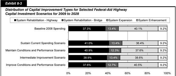
Exhibit 8-3 shows the distribution of spending by improvement type for each Federal-aid highway scenario and compares this distribution with actual spending in 2008. As noted above, capital spending on system enhancements amounts to 9.2 percent of each scenario’s investment total, consistent with the percentage of total capital spending on Federal-aid highways by all levels of government directed to these types of improvements in 2008. By design, the Sustain Current Spending scenario and the Intermediate Improvement scenario each allocates 13.4 percent of spending to the types of bridge improvements modeled in NBIAS (repair, rehabilitation, and replacement), which is the share of actual 2008 spending on Federal-aid highways that was directed to such improvements. In the other scenarios, the level of NBIAS-modeled investment is determined independently. The types of improvements modeled in HERS are reflected in the “System Rehabilitation – Highway” and “System Expansion” categories; the distribution between these categories in each scenario is based on an evaluation of the relative benefits and costs of potential investments in each area.

In 2008, 40.1 percent of capital outlay by all levels of government on Federal-aid highways was directed to system expansion. The Sustain Current Spending scenario reduces this share to 36.4 percent, while other scenarios maintain or increase this share at higher levels of spending. For example, the Improve Conditions and Performance scenario directs 40.5 percent of its total investment towards system expansion.

Exhibit 8-3. Distribution of Capital Improvement Types for Selected Federal-Aid Highway Capital Investment Scenarios for 2009 to 2028. Stacked bar chart showing percentages of capital spending by four improvement types for four Federal-aid highway scenarios and by baseline 2008 spending. For system rehabilitation of highways, the four scenarios would account for 37.6 to 41.0 percent, as compared with the 37.3 percent actual rate of 2008 spending. For system rehabilitation of bridges, the scenarios would account for 12.3 to 13.4 percent, as compared with the 13.4 percent actual rate of 2008 spending. For system expansion, the scenarios would account for 40.5 to 36.4 percent, as compared with the 40.1 percent actual rate of 2008 spending. For system enhancement, the scenarios each would account for 9.2 percent, equal to the 9.2 percent actual rate of 2008 spending. Sources: Highway Economic Requirements System and National Bridge Investment Analysis System.

Scenario Name	Average Annual Investment (Billions of 2008 Dollars)
Scenario Name	System Rehabilitation Highway¹	System Rehabilitation Bridge²	System Rehabilitation Total	System Expansion ³	System Enhancement	Total
Baseline 2008 Spending	$26.4	$9.4	$35.8	$28.3	$6.5	$70.6
Sustain Current Spending scenario	$29.0	$9.4	$38.4	$25.7	$6.5	$70.6
Maintain Conditions and Performance scenario	$32.7	$9.8	$42.6	$30.1	$7.4	$80.1
Intermediate Improvement scenario	$40.2	$13.8	$54.0	$39.9	$9.5	$103.5
Improve Conditions and Performance scenario	$50.7	$17.1	$67.8	$54.7	$12.4	$134.9
State of Good Repair benchmark⁴	$50.7	$17.1	$67.8

¹ Values shown correspond to amounts in Exhibit 7-5 in Chapter 7.
² Values shown correspond to amounts in Exhibit 7-18 in Chapter 7.
³ Values shown correspond to amounts in Exhibits 7-6 and 7-7 in Chapter 7.
⁴ The State of Good Repair benchmark is a subset of the Improve Conditions and Performance scenario.

Sources: Highway Economic Requirements System and National Bridge Investment Analysis System.

The Improve Conditions and Performance scenario directs $67.8 billion, or 50.3 percent, of the $134.9 billion in average annual spending it programs for Federal-aid highways towards the types of system rehabilitation actions reflected in the State of Good Repair benchmark. Although this level of investment falls short of the $70.6 billion of total capital spending on Federal-aid highways in 2008, it substantially exceeds the portion of that spending, $35.8 billion, that was used for system rehabilitation improvements. This suggests that the current backlog of cost-beneficial improvements to address pavement and bridge deficiencies is substantial, and that achieving a state of good repair on Federal-aid highways would require either a significant increase in overall highway and bridge investment, or a significant redistribution of investment from other types of improvements towards System Rehabilitation.

Sustain Current Spending Scenario

For the Sustain Current Spending scenario for Federal-aid highways, Exhibit 8-4 compares the scenario distribution of capital investments by improvement type and functional class with the corresponding actual distribution in 2008 (from Chapter 6; see Exhibit 6-10 and Exhibit 6-12). Due to the manner in which this scenario was constructed, the total percentage change identified for the “System Rehabilitation – Bridge,” “System Enhancement” and the “Total” columns in the table are automatically all zero, as are the values for individual functional classes in the “System Enhancement” column.

Although the Sustain Current Spending scenario for Federal-aid highways fixes average annual capital spending on these highways at the actual 2008 level, the portion of this spending it allocates to the “System Rehabilitation – Highway” category is 9.8 percent higher than the corresponding 2008 amount. Conversely, the allocation to “System Expansion” is 9.2 percent lower than the actual 2008 values. When it comes to the distribution of investment by highway functional class, the differences between the scenario and actual 2008 allocations are more pronounced. Relative to the corresponding actual 2008 amounts, the $14.3 billion of average annual investment on rural arterials and major collectors included in this scenario would represent a 47.4 percent decrease, while the $56.3 billion of average annual investment on urban arterials and collectors would represent a 29.8 percent increase.

Exhibit 8-4
Sustain Current Spending Scenario for Federal-Aid Highways: Distribution of Average Annual Investment for 2009 to 2028 Compared With Actual 2008 Spending, by Functional Class and Improvement Type
Average Annual National Investment on Federal-Aid Highways (Billions of 2008 Dollars)
Functional Class	System Rehabilitation Highway	System Rehabilitation Bridge	System Rehabilitation Total	System Expansion	System Enhancement	Total
Rural Arterials and Major Collectors
Interstate	$1.6	$0.6	$2.3	$1.5	$0.4	$4.2
Other Principal Arterial	$1.5	$0.5	$2.0	$0.7	$0.7	$3.4
Minor Arterial	$1.7	$0.5	$2.1	$0.4	$0.5	$3.0
Major Collector	$2.1	$0.8	$2.9	$0.2	$0.7	$3.7
Subtotal	$6.9	$2.4	$9.3	$2.7	$2.3	$14.3
Urban Arterials and Collectors
Interstate	$6.0	$2.6	$8.6	$11.5	$1.0	$21.1
Other Freeway and Expressway	$2.8	$1.0	$3.8	$4.5	$0.6	$8.9
Other Principal Arterial	$4.9	$1.6	$6.5	$3.1	$1.2	$10.8
Minor Arterial	$6.1	$1.3	$7.4	$2.7	$0.9	$11.0
Collector	$2.3	$0.5	$2.8	$1.1	$0.5	$4.4
Subtotal	$22.1	$7.0	$29.1	$23.0	$4.3	$56.3
Total, Federal-Aid Highways^*	$29.0	$9.4	$38.4	$25.7	$6.5	$70.6

Percent Above Actual 2008 Capital Spending on Federal-Aid Highways by All Levels of Government Combined
Functional Class	System Rehabilitation Highway	System Rehabilitation Bridge	System Rehabilitation Total	System Expansion	System Enhancement	Total
Rural Arterials and Major Collectors
Interstate	-50.3%	-3.6%	-42.4%	1.7%	0.0%	-28.1%
Other Principal Arterial	-63.5%	-32.8%	-58.5%	-85.1%	0.0%	-66.9%
Minor Arterial	-33.7%	-39.7%	-35.2%	-81.5%	0.0%	-47.8%
Major Collector	-16.7%	-30.1%	-20.8%	-82.4%	0.0%	-30.2%
Subtotal	-44.6%	-27.8%	-41.0%	-70.1%	0.0%	-47.4%
Urban Arterials and Collectors
Interstate	40.6%	0.7%	25.3%	82.5%	0.0%	49.0%
Other Freeway and Expressway	90.3%	164.2%	105.5%	105.5%	0.0%	91.7%
Other Principal Arterial	23.3%	7.6%	19.0%	-52.2%	0.0%	-18.1%
Minor Arterial	131.1%	45.8%	109.9%	-3.7%	0.0%	52.2%
Collector	41.1%	-32.0%	19.8%	-11.4%	0.0%	7.7%
Subtotal	58.1%	15.5%	45.2%	20.2%	0.0%	29.8%
Total, Federal-Aid Highways *	9.8%	0.0%	7.2%	-9.2%	0.0%	0.0%

^* The term “Federal-Aid Highways” refers to those portions of the road network that are generally eligible for Federal funding. Roads functionally classified as rural minor collectors, rural local, and urban local are excluded, although some types of Federal program funds can be used on such facilities.

Sources: Highway Economic Requirements System and National Bridge Investment Analysis System.

Overall, the Sustain Current Spending scenario for Federal-aid highways would reduce annual spending below the 2008 level for each rural functional class and for urban other principal arterials. Within the “System Rehabilitation – Highway” category, the same is true for each individual rural functional class, while the opposite holds for each urban functional class (i.e., the scenario spending would exceed the 2008 level). The results for the “System Rehabilitation – Bridges” category are similar, except that scenario spending would also be less than the 2008 level for bridges on urban collectors. For the “System Expansion” category, scenario spending would exceed the 2008 level significantly on the urban portion of the Interstate System and on other urban freeways and expressways, and slightly on the rural portion of the Interstate System; for all other functional systems, the scenario spending would be less than the 2008 level.

These differences between the scenario and actual allocations, while suggestive from a policy perspective, do not necessarily indicate misallocations of actual capital spending. Apart from the errors that may result from limitations of the HERS and NBIAS models and the associated databases, two other considerations argue for caution. First, the actual distribution of expenditures among improvement types and functional classes varies from year to year, and 2008 may be atypical in some respects. Second, even if annual highway and bridge investment were to continue on average at the 2008 level, changing circumstances would alter the economically optimal distribution of this spending. The actual distribution in 2008 could, therefore, make perfect economic sense and still differ significantly from the economically optimal distribution over the following 20 years.

Maintain Conditions and Performance Scenario

Exhibit 8-5 identifies the distribution of capital investments by improvement type and functional class for the Maintain Conditions and Performance scenario for Federal-aid highways. The $16.2 billion of capital investment on rural arterials and major collectors represents 20.2 percent of the $80.1 billion total average annual investment (by all levels of government combined) under this scenario. By design, the rural share of total system enhancement expenditures is 34.6 percent ($2.6 billion out of $7.4 billion), the same as the actual percentage in 2008. Rural roads receive in this scenario 10.2 percent of system expansion expenditures and 24.9 percent of system rehabilitation expenditures.

Exhibit 8-5
Maintain Conditions and Performance Scenario for Federal-Aid Highways: Distribution of Average Annual Investment for 2009 to 2028, by Functional Class and Improvement Type
Average Annual National Investment on Federal-Aid Highways (Billions of 2008 Dollars)
Functional Class	System Rehabilitation Highway	System Rehabilitation Bridge	System Rehabilitation Total	System Expansion	System Enhancement	Total
Rural Arterials and Major Collectors
Interstate	$1.8	$0.7	$2.4	$1.6	$0.5	$4.5
Other Principal Arterial	$1.8	$0.6	$2.4	$0.8	$0.8	$4.0
Minor Arterial	$1.9	$0.5	$2.4	$0.4	$0.5	$3.4
Major Collector	$2.6	$0.8	$3.4	$0.3	$0.8	$4.4
Subtotal	$8.1	$2.5	$10.6	$3.1	$2.6	$16.2
Urban Arterials and Collectors
Interstate	$6.5	$2.7	$9.2	$13.1	$1.1	$23.5
Other Freeway and Expressway	$3.1	$1.0	$4.1	$5.3	$0.7	$10.1
Other Principal Arterial	$5.6	$1.7	$7.3	$4.0	$1.4	$12.7
Minor Arterial	$6.7	$1.4	$8.1	$3.3	$1.1	$12.4
Collector	$2.7	$0.5	$3.2	$1.4	$0.6	$5.1
Subtotal	$24.7	$7.3	$32.0	$27.1	$4.8	$63.9
Total, Federal-Aid Highways ^*	$32.7	$9.8	$42.6	$30.1	$7.4	$80.1

Sources: Highway Economic Requirements System and National Bridge Investment Analysis System.

It is important to note that the goal of the Maintain Conditions and Performance scenario is to maintain average conditions and performance on a systemwide basis; the conditions and performance of individual functional classes may vary. Consequently, the dollar amount shown for each of the functional classes in Exhibit 8-5 does not represent the cost of maintaining the condition or performance of that functional class in isolation. A supplemental scenario is presented in Chapter 9 that identifies the costs of maintaining the conditions and performance of individual system components.

Intermediate Improvement Scenario

Exhibit 8-6 identifies the distribution of capital investments on Federal-aid highways by improvement type and functional class for the Intermediate Improvement scenario. The $20.6 billion of capital investment on rural arterials and major collectors represents 19.9 percent of the $103.5 billion total average annual investment under this scenario. Rural roads receive in this scenario 8.9 percent of system expansion expenditures and 25.3 percent of system rehabilitation expenditures. The relatively modest size of these rural shares reflects partly that rural minor collectors (along with rural local and urban local roads) are not classified as Federal-aid highways. As discussed in Chapter 2, while Federal-aid highways carry over five-sixths of total VMT, they account for less than one-quarter of total mileage. The system rehabilitation needs on the remaining three-quarters of total mileage are significant.

Exhibit 8-6
Intermediate Improvement Scenario for Federal-Aid Highways: Distribution of Average Annual Investment for 2009 to 2028, by Functional Class and Improvement Type
Average Annual National Investment on Federal-Aid Highways (Billions of 2008 Dollars)
Functional Class	System Rehabilitation Highway	System Rehabilitation Bridge	System Rehabilitation Total	System Expansion	System Enhancement	Total
Rural Arterials and Major Collectors
Interstate	$2.1	$0.9	$3.0	$1.7	$0.6	$5.3
Other Principal Arterial	$2.4	$0.7	$3.0	$1.0	$1.0	$5.0
Minor Arterial	$2.5	$0.7	$3.1	$0.4	$0.7	$4.2
Major Collector	$3.5	$1.0	$4.6	$0.4	$1.0	$6.0
Subtotal	$10.4	$3.3	$13.7	$3.6	$3.3	$20.6
Urban Arterials and Collectors
Interstate	$7.5	$3.6	$11.1	$17.0	$1.5	$29.6
Other Freeway and Expressway	$3.6	$1.4	$5.1	$7.3	$0.9	$13.3
Other Principal Arterial	$7.3	$2.5	$9.8	$5.6	$1.8	$17.1
Minor Arterial	$7.8	$2.2	$10.0	$4.4	$1.4	$15.7
Collector	$3.5	$0.8	$4.4	$2.1	$0.7	$7.2
Subtotal	$29.8	$10.6	$40.3	$36.4	$6.2	$82.9
Total, Federal-Aid Highways ^*	$40.2	$13.8	$54.0	$39.9	$9.5	$103.5

Sources: Highway Economic Requirements System and National Bridge Investment Analysis System.

Improve Conditions and Performance Scenario

In the Improve Conditions and Performance scenario for Federal-aid highways, total investment in these highways by all levels of government averages $134.9 billion per year, or nearly double the 2008 level of spending, but rural arterials and major collectors receive only $26.9 billion of this amount, or 1.3 percent less than in 2008. This stems mainly from a substantial reduction in funding for rural other principal arterials. As shown in Exhibit 8-7, this scenario would direct 15.2 percent more per year toward rural system rehabilitation than what was spent in 2008, but would direct 52.3 percent less toward rural system expansion. Among the urban functional classes, the scenario would more than triple the amount currently expended on other urban freeways and expressways; the scenario would more than double the amount currently expended on the urban portion of the Interstate System, urban minor arterials, and urban collectors.

Exhibit 8-7
Improve Conditions and Performance Scenario for Federal-Aid Highways: Distribution of Average Annual Investment for 2009 to 2028 Compared With Actual 2008 Spending, by Functional Class and Improvement Type
Average Annual National Investment on Federal-Aid Highways (Billions of 2008 Dollars)
Functional Class	System Rehabilitation Highway	System Rehabilitation Bridge	System Rehabilitation Total	System Expansion	System Enhancement	Total
Rural Arterials and Major Collectors
Interstate	$2.3	$1.1	$3.4	$2.0	$0.8	$6.2
Other Principal Arterial	$3.2	$0.8	$4.0	$1.3	$1.3	$6.6
Minor Arterial	$3.4	$0.8	$4.1	$0.5	$0.9	$5.6
Major Collector	$5.4	$1.2	$6.7	$0.6	$1.3	$8.5
Subtotal	$14.3	$3.8	$18.2	$4.4	$4.3	$26.9
Urban Arterials and Collectors
Interstate	$8.6	$4.3	$12.8	$21.8	$1.9	$36.5
Other Freeway and Expressway	$4.4	$1.7	$6.1	$9.9	$1.2	$17.2
Other Principal Arterial	$9.6	$3.2	$12.8	$9.0	$2.3	$24.0
Minor Arterial	$9.1	$3.0	$12.1	$6.5	$1.8	$20.3
Collector	$4.7	$1.1	$5.8	$3.2	$1.0	$9.9
Subtotal	$36.3	$13.2	$49.6	$50.3	$8.1	$108.0
Total, Federal-Aid Highways ^*	$50.7	$17.1	$67.8	$54.7	$12.4	$134.9

Percent Above Actual 2008 Capital Spending on Federal-Aid Highways by All Levels of Government Combined
Functional Class	System Rehabilitation Highway	System Rehabilitation Bridge	System Rehabilitation Total	System Expansion	System Enhancement	Total
Rural Arterials and Major Collectors
Interstate	-28.6%	58.9%	-13.6%	34.0%	91.0%	6.0%
Other Principal Arterial	-21.9%	-4.8%	-19.1%	-72.7%	91.0%	-36.5%
Minor Arterial	34.2%	-3.4%	25.1%	-72.6%	91.0%	-2.2%
Major Collector	116.7%	11.3%	84.4%	-43.4%	91.0%	60.2%
Subtotal	15.7%	13.4%	15.2%	-52.3%	91.0%	-1.3%
Urban Arterials and Collectors
Interstate	101.7%	63.0%	86.9%	244.4%	91.0%	157.3%
Other Freeway and Expressway	198.9%	348.0%	229.6%	351.0%	91.0%	268.7%
Other Principal Arterial	142.9%	112.5%	134.6%	36.5%	91.0%	81.9%
Minor Arterial	244.3%	238.6%	242.9%	133.2%	91.0%	181.2%
Collector	183.6%	64.8%	148.9%	151.6%	91.0%	142.6%
Subtotal	160.3%	118.8%	147.7%	163.0%	91.0%	148.9%
Total, Federal-Aid Highways *	92.3%	81.0%	89.3%	93.1%	91.0%	91.0%

Sources: Highway Economic Requirements System and National Bridge Investment Analysis System.

Overall, the average annual investment level under the Improve Conditions and Performance scenario for Federal-aid highways is 91.0 percent higher than the actual amount spent in 2008; spending on system enhancements for each functional class was assumed to grow by this same percentage. System expansion expenditures under this scenario are 93.1 percent higher than in 2008, while system rehabilitation expenditures are 89.3 percent higher.

Systemwide Scenarios

As discussed in Chapter 7 (Exhibit 7-1), the functional classes not counted as Federal-aid highways—rural minor collectors, rural local roads, and urban local roads—received $17.2 billion out of the $91.1 billion invested systemwide in highways and bridges in 2008. Since these functional classes are not represented in the HPMS sample, they are not modeled in HERS. Adding this $17.2 billion to the $6.5 billion spent on system enhancements to Federal-aid highways means that $23.7 billion, or 26.0 percent, of systemwide capital spending was in the residual category not modeled by HERS or NBIAS.

Exhibit 8-8 summarizes the derivation of the systemwide scenarios. Each scenario links back to a specific funding level identified in the HERS and NBIAS analyses presented in Chapter 7. In computing the average annual investment levels over 20 years, the combined projections for the capital spending from the two models were adjusted upwards so that the non-modeled capital improvement types would remain at 26.0 percent of the total cost of each scenario, consistent with their share in 2008. The HERS-derived components of the systemwide scenarios are identical to those identified in Exhibit 8-1 for the Federal-aid highway scenarios. However, the NBIAS-derived components of the systemwide scenarios are different, as sufficient data available are available through the National Bridge Inventory to develop separate estimates, applying the scenario criteria to all bridges rather than just the subset of bridges on Federal-aid highways.

In 2008, $3.4 billion of the $12.8 billion in total bridge rehabilitation spending by all levels of government was directed to bridges on non-Federal-Aid highways. For the systemwide Sustain Current Spending scenario, this additional funding is available for NBIAS to direct to bridges on or off Federal-aid highways, as determined by the optimization algorithms in NBIAS. (In fact, the model would direct 85.4 percent of the $12.8 billion to bridges on Federal-aid highways under this scenario, while only 73.7 percent of this amount was directed to such bridges in 2008.)

The average annual investment level for the systemwide Maintain Conditions and Performance scenario is $101.0 billion. For bridge rehabilitation, NBIAS projects that maintaining the systemwide economic backlog of investment at its 2008 level would require investing over 20 years at an average annual level of only $11.9 billion in 2008 dollars, which is below the $12.8 billion spent in 2008. In the scenario, this reduction in average annual spending would be attained with spending on real expenditures on bridge rehabilitation decreasing 0.70 percent per year. In contrast, Exhibit 8-1 showed that maintaining the economic backlog for bridges on Federal-aid highways only would require rehabilitation spending on these bridges to increase. In combination, these findings suggest that the distribution of bridge spending in 2008 was somewhat better aligned with addressing long-term bridge needs off Federal-aid highways than on Federal-aid highways. (These findings are only suggestive because the modeling process entails many uncertainties and the 2008 spending data are partially estimated for some functional classes).

Exhibit 8-8
Definitions of Selected Systemwide Capital Investment Scenarios, and Average Annual Investment Levels for 2009 to 2028 Associated With Scenario Components
Scenario Name and Description	Scenario Component (Source of Estimate)¹	Component Share of 2008 Capital Outlay	Annual Percent Change in Spending vs. 2008	Minimum BCR	Average Annual Capital Investment on All Roads
Scenario Name and Description	Scenario Component (Source of Estimate)¹	Component Share of 2008 Capital Outlay	Annual Percent Change in Spending vs. 2008	Minimum BCR	Billions of 2008 Dollars	Percent of Total
Sustain Current Spending scenario (Sustain spending at base year levels in constant dollar terms.)	HERS²	60.0%	0.00%	2.42	$54.7	60.0%
Sustain Current Spending scenario (Sustain spending at base year levels in constant dollar terms.)	NBIAS³	14.0%	0.00%		$12.8	14.0%
Sustain Current Spending scenario (Sustain spending at base year levels in constant dollar terms.)	Other	26.0%			$23.7	26.0%
Sustain Current Spending scenario (Sustain spending at base year levels in constant dollar terms.)	Total	100.0%			$91.1	100.0%
Maintain Conditions and Performance scenario (Maintain average speed and the economic bridge investment backlog at 2008 levels.)	HERS ²	60.0%	1.31%	2.02	$62.9	62.3%
Maintain Conditions and Performance scenario (Maintain average speed and the economic bridge investment backlog at 2008 levels.)	NBIAS ³	14.0%	-0.70%		$11.9	11.8%
Maintain Conditions and Performance scenario (Maintain average speed and the economic bridge investment backlog at 2008 levels.)	Other	26.0%			$26.2	26.0%
Maintain Conditions and Performance scenario (Maintain average speed and the economic bridge investment backlog at 2008 levels.)	Total	100.0%			$101.0	100.0%
Intermediate Improvement scenario (Invest in projects with benefit-cost ratios as low as 1.5 and reduce the economic bridge investment backlog.)	HERS ²	60.0%	3.51%	1.50	$80.1	60.0%
Intermediate Improvement scenario (Invest in projects with benefit-cost ratios as low as 1.5 and reduce the economic bridge investment backlog.)	NBIAS ³	14.0%	3.51%		$18.7	14.0%
Intermediate Improvement scenario (Invest in projects with benefit-cost ratios as low as 1.5 and reduce the economic bridge investment backlog.)	Other	26.0%			$34.7	26.0%
Intermediate Improvement scenario (Invest in projects with benefit-cost ratios as low as 1.5 and reduce the economic bridge investment backlog.)	Total	100.0%			$133.5	100.0%
Improve Conditions and Performance scenario (Invest in all cost-beneficial projects and eliminate the economic bridge investment backlog.)	HERS ²	60.0%	5.90%	1.00	$105.4	62.0%
Improve Conditions and Performance scenario (Invest in all cost-beneficial projects and eliminate the economic bridge investment backlog.)	NBIAS ³	14.0%	4.31%		$20.5	12.1%
Improve Conditions and Performance scenario (Invest in all cost-beneficial projects and eliminate the economic bridge investment backlog.)	Other	26.0%			$44.2	26.0%
Improve Conditions and Performance scenario (Invest in all cost-beneficial projects and eliminate the economic bridge investment backlog.)	Total	100.0%			$170.1	100.0%

¹ Each scenario consists of three separately estimated components. The components derived from HERS and NBIAS represent the combined investment by all levels of government associated with achieving the scenario goals identified. The third scenario component, identified as “Other,” represents other types of capital spending beyond those modeled in HERS or NBIAS; each scenario assumes that the percentage of total spending on these nonmodeled items in the future will be the same as the actual percentage in 2008.
² The scenario components derived from HERS are directly linked to the analyses presented in Exhibits 7-3 through 7-10 in Chapter 7; these components can be cross-referenced to the exhibits using either the annual percent change in spending relative to 2008, or the minimum BCR identified in this table.
³ The scenario components derived from NBIAS are directly linked to the analysis presented in Exhibit 7-17 in Chapter 7; these components can be cross-referenced to this exhibit using the annual percent change in spending relative to 2008 identified in this table.

Sources: Highway Economic Requirements System and National Bridge Investment Analysis System.

The average annual investment levels for the 20-year period through 2028 for the systemwide Intermediate Improvement scenario and the systemwide Improve Conditions and Performance scenario are $133.5 billion and $170.1 billion, respectively. These figures are stated in constant 2008 dollars (as are all of the other scenario investment levels presented in this chapter, as stated earlier).

It is important to note that these scenarios are intended to be illustrative, and any number of alternative scenarios based on different BCR cutoff points, performance targets, or funding targets could be constructed that would be equally valid from a technical perspective.

Systemwide Scenario Impacts and Comparison with 2008 Spending

Exhibit 8-9 compares the systemwide scenarios with 2008 spending. The average annual investment level associated with the Maintain Conditions and Performance scenario is 10.8 percent higher than actual spending by all levels of government on capital improvements to highways and bridges in 2008; the comparable “gap” between the Improve Conditions and Performance scenario and 2008 spending is 86.6 percent.

Exhibit 8-9
Selected Systemwide Highway Capital Investment Scenarios for 2009 to 2028: Comparisons With 2008 Spending and Projected Systemwide Highway Performance Indicators
Comparison Parameter	Sustain Current Spending Scenario	Maintain Conditions & Performance Scenario	Intermediate Improvement Scenario	Improve Conditions & Performance Scenario
Comparison of Scenarios With 2008 Spending
Average Annual Investment (Billions of 2008 Dollars)	$91.1	$101.0	$133.5	$170.1
Difference Relative to 2008 Spending (Billions of 2008 Dollars)	$0.0	$9.8	$42.4	$78.9
Percent Difference Relative to 2008 Spending	0.0%	10.8%	46.5%	86.6%
Annual Percent Increase to Support Scenario Investment¹	0.00%	0.97%	3.51%	5.62%
Projected Impacts of Scenarios on All Roads²
Percent Change in Economic Bridge Investment Backlog (2028 vs. 2008)³	-11.2%	0.0%	-79.1%	-100.0%

¹ This percentage represents the annual percent change relative to 2008 that would be required to achieve the average annual funding level specified for the scenario in constant dollar terms. Additional increases in nominal dollar terms would be needed to offset the impact of future inflation.
² Systemwide performance information for pavement condition and congestion is not available, as the HERS analysis is limited to Federal-aid highways for which HPMS sample data are collected by the FHWA. See Exhibit 8-2 for performance information on Federal-aid highways. Bridge performance information is available on a systemwide basis, as the NBI includes data for all bridges over 20 feet in length.
³ Values shown correspond to amounts in Exhibit 7-17 in Chapter 7.

Sources: Highway Economic Requirements System and National Bridge Investment Analysis System.

Exhibit 8-9 also shows the projected impacts on the economic backlog of bridge rehabilitation projects in 2028. For the other conditions and performance indicators, which relate to speed, delay, or pavement condition, the only projections available for this analysis come from the HERS simulations, which cover the Federal-Aid highways alone. Hence, these indicators are absent from Exhibit 8-9, where the focus is systemwide. The Intermediate Improvement scenario projects that the economic investment backlog in 2028 will be 79.1 percent lower than in 2008, while the Sustain Current Spending scenario (in which bridge spending is higher than in the Maintain Conditions and Performance scenario, as noted above) projects an 11.2 percent reduction. For the other two scenarios, the scenario assumptions ensure that the backlog disappears by 2028 (Improve Conditions and Performance scenario) or remains at its 2008 level (Maintain Conditions and Performance scenario).

Systemwide Scenario Estimates by Improvement Type

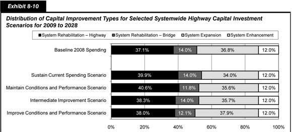
Exhibit 8-10 shows the distribution of highway capital spending by improvement type for each systemwide scenario, as well as the corresponding distribution of actual systemwide spending by all levels of government) in 2008. A comparison of this distribution with that shown in Exhibit 8-3 reveals that the percentage allocations to system expansion are typically a few points lower, and those to system enhancements are typically a few points higher in the systemwide scenarios than in the comparable Federal-aid highway scenarios; these differences primarily reflect corresponding differences in the base year spending patterns. In 2008, the system expansion share of capital spending was 40.1 percent of on Federal-aid highways and 36.8 percent systemwide, while the system enhancement shares were 9.2 percent on Federal-aid highways versus 12.0 percent systemwide.

Exhibit 8-10. Distribution of Capital Improvement Types for Selected Systemwide Highway Capital Investment Scenarios for 2009 to 2028. Stacked bar chart showing percentages of capital spending by four improvement types for four systemwide highway scenarios and by baseline 2008 spending. For system rehabilitation of highways, the four scenarios would account for 38.0 to 40.6 percent, as compared with the 37.1 percent actual rate of 2008 spending. For system rehabilitation of bridges, the scenarios would account for 11.8 to 14.0 percent, as compared with the 14.0 percent actual rate of 2008 spending. For system expansion, the scenarios would account for 34.0 to 37.9 percent, as compared with the 36.8 percent actual rate of 2008 spending. For system enhancement, the scenarios each would account for 12.0 percent, equal to the 12.0 percent actual rate of 2008 spending. Sources: Highway Economic Requirements System and National Bridge Investment Analysis System.

Scenario Name	Average Annual Investment (Billions of 2008 Dollars)
Scenario Name	System Rehabilitation Highway¹	System Rehabilitation Bridge²	System Rehabilitation Total	System Expansion ¹	System Enhancement	Total
Baseline 2008 Spending	$33.8	$12.8	$46.6	$33.6	$11.0	$91.1
Sustain Current Spending scenario	$36.4	$12.8	$49.2	$31.0	$11.0	$91.1
Maintain Conditions and Performance scenario	$41.0	$11.9	$52.9	$36.0	$12.1	$101.0
Intermediate Improvement scenario	$51.1	$18.7	$69.9	$47.6	$16.1	$133.5
Improve Conditions and Performance scenario	$64.6	$20.5	$85.1	$64.5	$20.5	$170.1
State of Good Repair benchmark³	$64.6	$20.5	$85.1

¹ Values shown include estimates for functional classes not modeled in HERS, and thus do not directly correspond to the exhibits presented in Chapter 7.
² Values shown correspond to amounts in Exhibit 7-17 in Chapter 7.
³ The State of Good Repair benchmark is a subset of the Improve Conditions and Performance scenario.

Sources: Highway Economic Requirements System and National Bridge Investment Analysis System.

Of the $170.1 billion average annual investment level for the systemwide Improve Conditions and Performance scenario, $85.1 billion (50.1 percent) would be directed towards the types of system rehabilitation actions reflected in the State of Good Repair benchmark. Although this level of investment is below the $91.1 billion spent for all highway capital improvements in 2008, it significantly exceeds the $46.6 billion spent in 2008 for system rehabilitation improvements.

National Highway System Scenarios

Exhibit 8-11 describes the derivation of the investment levels for each of four NHS capital investment scenarios, which each draw from the HERS and NBIAS analyses presented in Chapter 7. (The footnotes in Exhibit 8-11 identify the specific Chapter 7 exhibits to which the scenarios are linked.) Each scenario covers the 20-year period from 2008 to 2028, and the investment levels shown are all “real,” stated in constant 2008 dollars.

Exhibit 8-11
Definitions of Selected NHS Capital Investment Scenarios, and Average Annual Investment Levels for 2009 to 2028 Associated With Scenario Components
Scenario Name and Description	Scenario Component (Source of Estimate)¹	Component Share of 2008 Capital Outlay	Annual Percent Change in Spending vs. 2008	Minimum BCR	Average Annual Capital Investment on All Roads
Scenario Name and Description	Scenario Component (Source of Estimate)¹	Component Share of 2008 Capital Outlay	Annual Percent Change in Spending vs. 2008	Minimum BCR	Billions of 2008 Dollars	Percent of Total
Sustain Current Spending scenario (Sustain spending at base year levels in constant dollar terms.)	HERS²	79.3%	0.00%	2.26	$33.3	79.3%
Sustain Current Spending scenario (Sustain spending at base year levels in constant dollar terms.)	NBIAS³	12.9%	0.00%		$5.4	12.9%
Sustain Current Spending scenario (Sustain spending at base year levels in constant dollar terms.)	Other	7.8%			$3.3	7.8%
Sustain Current Spending scenario (Sustain spending at base year levels in constant dollar terms.)	Total	100.0%			$42.0	100.0%
Maintain Conditions and Performance scenario (Maintain average speed and the economic bridge investment backlog at 2008 levels.)	HERS ²	79.3%	-0.87%	2.55	$30.4	78.4%
Maintain Conditions and Performance scenario (Maintain average speed and the economic bridge investment backlog at 2008 levels.)	NBIAS ³	12.9%	-0.09%		$5.4	13.8%
Maintain Conditions and Performance scenario (Maintain average speed and the economic bridge investment backlog at 2008 levels.)	Other	7.8%			$3.0	7.8%
Maintain Conditions and Performance scenario (Maintain average speed and the economic bridge investment backlog at 2008 levels.)	Total	100.0%			$38.9	100.0%
Intermediate Improvement scenario (Invest in projects with benefit-cost ratios as low as 1.5 and reduce the economic bridge investment backlog.)	HERS ²	79.3%	2.80%	1.50	$45.1	79.3%
Intermediate Improvement scenario (Invest in projects with benefit-cost ratios as low as 1.5 and reduce the economic bridge investment backlog.)	NBIAS ³	12.9%	2.80%		$7.3	12.9%
Intermediate Improvement scenario (Invest in projects with benefit-cost ratios as low as 1.5 and reduce the economic bridge investment backlog.)	Other	7.8%			$4.4	7.8%
Intermediate Improvement scenario (Invest in projects with benefit-cost ratios as low as 1.5 and reduce the economic bridge investment backlog.)	Total	100.0%			$56.9	100.0%
Improve Conditions and Performance scenario (Invest in all cost-beneficial projects and eliminate the economic bridge investment backlog.)	HERS ²	79.3%	4.91%	1.00	$57.3	79.8%
Improve Conditions and Performance scenario (Invest in all cost-beneficial projects and eliminate the economic bridge investment backlog.)	NBIAS ³	12.9%	4.48%		$8.9	12.4%
Improve Conditions and Performance scenario (Invest in all cost-beneficial projects and eliminate the economic bridge investment backlog.)	Other	7.8%			$5.6	7.8%
Improve Conditions and Performance scenario (Invest in all cost-beneficial projects and eliminate the economic bridge investment backlog.)	Total	100.0%			$71.8	100.0%

¹ Each scenario consists of three separately estimated components. The components derived from HERS and NBIAS represent the combined investment by all levels of government associated with achieving the scenario goals identified. The third scenario component, identified as “Other,” represents other types of capital spending beyond those modeled in HERS or NBIAS; each scenario assumes that the percentage of total spending on these nonmodeled items in the future will be the same as the actual percentage in 2008.
² The scenario components derived from HERS are directly linked to the analyses presented in Exhibits 7-11 through 7-13 in Chapter 7; these components can be cross-referenced to the exhibits using either the annual percent change in spending relative to 2008, or the minimum BCR identified in this table.
³ The scenario components derived from NBIAS are directly linked to the analysis presented in Exhibit 7-19 in Chapter 7; these components can be cross-referenced to this exhibit using the annual percent change in spending relative to 2008 identified in this table.

Sources: Highway Economic Requirements System and National Bridge Investment Analysis System.

All levels of government spent a combined $42.0 billion on capital improvements to highways and bridges on the NHS in 2008; as shown in Exhibit 8-11, $33.3 billion of this total (79.3 percent) was used for the type of capital improvements modeled in HERS, $5.4 billion (12.9 percent) for types of improvements modeled in NBIAS, and $3.3 billion (7.8 percent) for other types of capital improvements. By definition, these amounts match the average annual investment levels for the NHS Sustain Current Spending scenario. Each of the other NHS scenarios assume that the share of average annual investment directed towards non-modeled capital improvements will remain at the 2008 level of 7.6 percent.

Exhibit 8-11 also identifies the annual rates of real spending growth associated with the HERS and NBIAS components of each scenario. For the NHS Maintain Conditions and Performance scenario, each of these growth rates is negative, indicating that 2008 spending levels are higher than the amount required over 20 years to meet the performance objectives of this scenario (maintain average speed at 2008 levels and prevent the economic bridge investment backlog from rising above its 2008 level in constant dollar terms). The average annual investment level associated with the NHS Maintain Conditions and Performance scenario is $38.9 billion. The HERS-derived component of this scenario would address all potential capital improvements with a BCR of 2.55 or higher; the comparable value for the Sustain Current Spending scenario is 2.26 (because the model implements improvements in descending order of their BCRs, scenarios with higher investment levels will have lower minimum BCRs).

Addressing all potential improvements with BCRs of 1.50 or higher as computed by HERS would require annual increase in related spending of 2.80 percent per year over 20 years. Applying this same growth rate to all other types of capital spending generates the estimated average annual investment level of $56.9 billion for the NHS Intermediate Improvement scenario.

The goal of the Improve Conditions and Performance scenario is to address all potential highway and bridge improvements with a BCR of 1.0 or higher. As shown in Exhibit 8-11, HERS projects that meeting this goal would require capital spending on the NHS to increase annually by 4.91 percent and 4.48 percent for the types of NHS improvements modeled in HERS and NBIAS, respectively. Funding these cost-beneficial improvements, while keeping the share of non-modeled spending at its 2008 share of 7.8 percent of total spending, would require an average annual investment of $71.8 billion for capital improvements to NHS highways and bridges over 20 years, stated in constant 2008 dollars.

NHS Scenario Impacts and Comparison with 2008 Spending

Exhibit 8-12 compares the capital investment levels associated with each of the selected NHS scenarios with actual NHS capital spending in 2008 and presents the associated projections for summary measures of conditions and performance. By definition, the NHS Maintain Conditions and Performance scenario will result in zero change between 2008 and 2028 in average speed and in the economic bridge investment backlog. The other non-targeted measures include the average IRI, projected to decrease by 9.2 percent (consistent with an improvement in physical conditions), and average delay per VMT, projected to increase by 0.7 percent (consistent with a worsening of operational performance). The $38.9 billion average annual investment level for the NHS Maintain Conditions and Performance scenario is 7.6 percent below the $42.0 billion of actual capital spending on the NHS in 2008. The scenario assumes that this reduction in investment would be achieved with spending decreasing by 0.76 percent per year over 20 years. This result, combined with the finding presented in Exhibit 8-1 that an increase in investment would be needed to achieve the objectives of this scenario for Federal-aid highways, suggests that the distribution spending in 2008 was somewhat better aligned with addressing long-term highway and bridge needs on the NHS than off of the NHS.

As the NHS Sustain Current Spending scenario has a higher average annual investment level than the NHS Maintain Conditions and Performance scenario, it is projected to result in improvements to NHS conditions and performance. As shown in Exhibit 8-12, relative to values in the 2008 base year, the projections are for average speeds to increase by 0.8 percent. Average delay and average IRI are also projected to decline, consistent with general improvements to operational performance and pavement conditions. The size of the economic bridge investment backlog is also projected to be reduced by approximately 1.8 percent over 20 years.

Exhibit 8-12
Selected NHS Capital Investment Scenarios for 2009 to 2028: Comparisons With 2008 Spending and Projected NHS Performance Indicators
Comparison Parameter	Sustain Current Spending Scenario	Maintain Conditions & Performance Scenario	Intermediate Improvement Scenario	Improve Conditions & Performance Scenario
Comparison of Scenarios With 2008 Spending
Average Annual Investment (Billions of 2008 Dollars)	$42.0	$38.9	$56.9	$71.8
Difference Relative to 2008 Spending (Billions of 2008 Dollars)	$0.0	-$3.2	$14.9	$29.7
Percent Difference Relative to 2008 Spending	0.0%	-7.6%	35.3%	70.7%
Annual Percent Increase to Support Scenario Investment¹	0.00%	-0.76%	2.80%	4.85%
Projected Impacts of Scenarios on Federal-Aid Highways
Percent Change in Average Speed (2028 vs. 2008)²	0.8%	0.0%	3.6%	5.7%
Percent of VMT on Roads With Good Ride Quality, 2028 ³	73.6%	70.8%	83.0%	89.6%
Percent of VMT on Roads With Acceptable Ride Quality, 2028 ³	93.6%	92.8%	95.8%	97.4%
Percent Change in Average IRI (2028 vs. 2008) ³	-13.4%	-9.2%	-25.2%	-33.6%
Percent Change in Average Delay per VMT (2028 vs. 2008) ²	-2.9%	0.7%	-16.1%	-26.3%
Percent Change in Economic Bridge Investment Backlog (2028 vs. 2008)⁴	-1.8%	0.0%	-56.7%	-100.0%

¹This percentage represents the annual percent change relative to 2008 that would be required to achieve the average annual funding level specified for the scenario in constant dollar terms. Additional increases in nominal dollar terms would be needed to offset the impact of future inflation.
² Values shown correspond to amounts in Exhibit 7-13 in Chapter 7.
³ Values shown correspond to amounts in Exhibit 7-12 in Chapter 7. Reductions in average pavement roughness (IRI) tranlate into improved ride quality.
⁴ Values shown correspond to amounts in Exhibit 7-19 in Chapter 7.

Sources: Highway Economic Requirements System and National Bridge Investment Analysis System.

Under the NHS Improve Conditions and Performance scenario, the percent of NHS VMT on pavements with good ride quality is projected to rise to 89.6 percent, while the percent of VMT on pavements with acceptable ride quality reaches 97.4 percent. By definition, this scenario would eliminate the economic bridge investment backlog on the NHS by 2028; it is also projected to increase average speeds by 5.7 percent by that date relative to 2008. Average pavement roughness is projected to be reduced by 33.6 percent on the NHS, while average delay per VMT on the NHS would decrease by 26.3 percent by 2028. The potential for reductions to average delay per VMT is relatively large (relative to the values identified for Federal-aid highways in Exhibit 8-3) because strategic investments in NHS System Expansion, coupled with the continued deployment of Intelligent Transportation Systems on a growing share of the NHS, has the potential to significantly improve operating performance.

Can highway capacity be expanded without either building new roads and bridges or adding new lanes to existing facilities?

Yes. The “System Expansion” investment levels identified in this chapter reflect a need for a certain amount of effective highway capacity, which could be met by traditional expansion or by other means. In some cases, effective highway capacity can be increased by improving the utilization of the existing infrastructure rather than by expanding it. The investment scenario estimates presented in this report consider the impact of some of the most significant operations strategies and deployments on highway system performance; these relationships are described in more detail in Appendix A. The potential implications of accelerating the deployment of operations strategies or implementing congestion pricing are explored in Chapter 9.

The methodology used to estimate the system expansion component of the investment scenarios also allows high-cost capacity improvements to be considered as an option for segments with high volumes of projected future travel, but have been coded by States as infeasible for conventional widening. Conceptually, such improvements might consist of new highways or bridges in the same corridor (or tunneling or double-decking on an existing alignment), but the capacity upgrades could also come through other transportation improvements, such as a parallel fixed-guideway transit line or mixed-use, high-occupancy vehicle/bus lanes.

The average annual investment level for NHS Improve Conditions and Performance scenario of $71.8 billion is 70.7 percent higher than actual spending on the NHS in 2008. NHS spending would need to increase by 4.85 percent per year over 20 years to reach this average annual level. Achieving the less-ambitious objectives of the NHS Intermediate Improvement scenario would require an annual spending increase of 2.80 percent through 2028.

NHS Scenario Estimates by Improvement Type

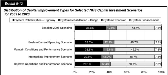
Exhibit 8-13 compares the distribution of highway and bridge capital outlay among the 20-year NHS capital investment scenarios and with actual NHS spending in 2008. As noted above, each scenario was derived in such a manner that capital spending on non-modeled system enhancement would equal 7.8 percent of the average annual investment level for that scenario. The share of the Sustain Current Spending scenario and the Intermediate Improvement scenario capital spending directed to bridge system rehabilitation matches the 2008 percentage of 12.9 percent by design; for the other scenarios, the level of NBIAS-modeled investment is determined independently.

Exhibit 8-13. Distribution of Capital Improvement Types for Selected NHS Capital Investment Scenarios for 2009 to 2028. Stacked bar chart showing percentages of capital spending by four improvement types for four National Highway System scenarios and by baseline 2008 spending. For system rehabilitation of highways, the four scenarios would account for 29.1 to 32.8 percent, as compared with the 35.6 percent actual rate of 2008 spending. For system rehabilitation of bridges, the scenarios would account for 12.4 to 13.8 percent, as compared with the 12.9 percent actual rate of 2008 spending. For system expansion, the scenarios would account for 45.6 to 50.7 percent, as compared with the 43.7 percent actual rate of 2008 spending. For system enhancement, the scenarios each would account for 7.8 percent, equal to the 7.8 percent actual rate of 2008 spending. Sources: Highway Economic Requirements System and National Bridge Investment Analysis System.

Scenario Name	Average Annual Investment (Billions of 2008 Dollars)
Scenario Name	System Rehabilitation Highway¹	System Rehabilitation Bridge²	System Rehabilitation Total	System Expansion ³	System Enhancement	Total
Baseline 2008 Spending	$15.0	$5.4	$20.4	$18.4	$3.3	$42.0
Sustain Current Spending scenario	$13.7	$5.4	$19.1	$19.6	$3.3	$42.0
Maintain Conditions and Performance scenario	$12.7	$5.4	$18.1	$17.7	$3.0	$38.9
Intermediate Improvement scenario	$17.4	$7.3	$24.7	$27.7	$4.4	$56.9
Improve Conditions and Performance scenario	$20.9	$8.9	$29.8	$36.4	$5.6	$71.8
State of Good Repair benchmark⁴	$20.9	$8.9	$29.8

¹ Values shown correspond to amounts in Exhibit 7-12 in Chapter 7.
² Values shown correspond to amounts in Exhibit 7-19 in Chapter 7.
³ Values shown correspond to amounts in Exhibit 7-13 in Chapter 7.
⁴ The State of Good Repair benchmark is a subset of the Improve Conditions and Performance scenario.

Sources: Highway Economic Requirements System and National Bridge Investment Analysis System.

In each of the four scenarios, system expansion receives a higher share of future investment than the 43.7 percent actually received in 2008. The NHS Sustain Current Spending scenario increases this share to 46.7 percent, while the NHS Improve Conditions and Performance scenario would increase it further to 50.7 percent.

Of the $71.8 billion average annual investment level for the NHS Improve Conditions and Performance scenario, $29.8 billion (41.5 percent) would be directed towards the types of system rehabilitation actions reflected in the State of Good Repair benchmark. This benchmark level is 46.1 percent more than the $20.4 billion spent by all levels of government on capital improvements of this nature on the NHS in 2008. While achieving this objective would be ambitious, this funding gap is relatively smaller than many of the others presented in this chapter.

Interstate System Scenarios

The average annual investment levels shown for the Interstate System Sustain Current Spending scenario are identified in Exhibit 8-14 and are consistent with the 2008 Interstate System spending figures identified in Chapter 7 (see Exhibit 7-1). This scenario assumes the continuation of the percentage splits in spending among HERS-modeled, NBIAS-modeled, and non-modeled improvement types. Of the $20.0 billion of capital investment on the Interstate System in 2008, approximately $15.3 billion (or 76.4 percent) was used for types of improvements modeled in HERS, including pavement resurfacing, pavement reconstruction, and capacity additions to the existing highway and bridge network. Approximately $3.3 billion (or 16.4 percent) was used for types of bridge repair, rehabilitation, and replacement improvements modeled in NBIAS. The remaining $1.4 billion (or 7.1 percent) went for types of capital improvements not currently addressed by either HERS or NBIAS, including various safety enhancements, environmental enhancements, and traffic operations improvements.

Each of the Interstate System scenarios presented in Exhibit 8-14 assumes that the share of average annual investment directed towards non-modeled capital improvements will remain at the 2008 level of 7.1 percent. Consequently, the amounts identified as “other” capital spending in Exhibit 8-14 are proportionally larger or smaller than the 2008 spending level of $1.2 billion based on the change in modeled spending relative to the 2008 baseline. The footnotes in Exhibit 8-14 identify the exhibits in Chapter 7 to which the HERS-modeled and NBIAS-modeled components of each scenario are linked.

As shown in Exhibit 8-14, the average annual investment level for the Interstate System Maintain Conditions and Performance scenario for 2009 to 2028 is $24.3 billion, stated in constant 2008 dollars. The HERS-modeled component of this total is $19.3 billion; this level of investment could be achieved if spending on the types of capital improvements modeled in HERS were to increase by 2.17 percent annually in real terms during this 20-year period over the base year 2008 level of $15.3 billion. This finding, combined with the finding presented in Exhibit 8-11 that the objectives of the NHS version of this scenario component could be achieved without increasing related NHS spending above its 2008 level, suggests that the distribution of spending in 2008 was somewhat better aligned with addressing long-term highway needs on the portion of the NHS that is off the Interstate System than is on the Interstate System. The average annual investment level associated with the NBIAS-modeled component of the Interstate System Maintain Conditions and Performance scenario of $3.2 billion is slightly below the amount actually spent for related types of capital improvements in 2008.

Exhibit 8-14
Definitions of Selected Interstate Highway System Capital Investment Scenarios, and Average Annual Investment Levels for 2009 to 2028 Associated With Scenario Components
Scenario Name and Description	Scenario Component (Source of Estimate)¹	Component Share of 2008 Capital Outlay	Annual Percent Change in Spending vs. 2008	Minimum BCR	Average Annual Capital Investment on Interstate Highways
Scenario Name and Description	Scenario Component (Source of Estimate)¹	Component Share of 2008 Capital Outlay	Annual Percent Change in Spending vs. 2008	Minimum BCR	Billions of 2008 Dollars	Percent of Total
Sustain Current Spending scenario (Sustain spending at base year levels in constant dollar terms.)	HERS²	76.4%	0.00%	2.90	$15.3	76.4%
Sustain Current Spending scenario (Sustain spending at base year levels in constant dollar terms.)	NBIAS³	16.4%	0.00%		$3.3	16.4%
Sustain Current Spending scenario (Sustain spending at base year levels in constant dollar terms.)	Other	7.1%			$1.4	7.1%
Sustain Current Spending scenario (Sustain spending at base year levels in constant dollar terms.)	Total	100.0%			$20.0	100.0%
Maintain Conditions and Performance scenario (Maintain average speed and the economic bridge investment backlog at 2008 levels.)	HERS ²	76.4%	2.17%	2.63	$19.3	79.5%
Maintain Conditions and Performance scenario (Maintain average speed and the economic bridge investment backlog at 2008 levels.)	NBIAS ³	16.4%	-0.18%		$3.2	13.3%
Maintain Conditions and Performance scenario (Maintain average speed and the economic bridge investment backlog at 2008 levels.)	Other	7.1%			$1.7	7.1%
Maintain Conditions and Performance scenario (Maintain average speed and the economic bridge investment backlog at 2008 levels.)	Total	100.0%			$24.3	100.0%
Intermediate Improvement scenario (Invest in projects with benefit-cost ratios as low as 1.5 and reduce the economic bridge investment backlog.)⁴	HERS ²	76.4%	5.54%	1.50	$28.3	78.1%
Intermediate Improvement scenario (Invest in projects with benefit-cost ratios as low as 1.5 and reduce the economic bridge investment backlog.)	NBIAS ³	16.4%	4.39%		$5.3	14.7%
Intermediate Improvement scenario (Invest in projects with benefit-cost ratios as low as 1.5 and reduce the economic bridge investment backlog.)	Other	7.1%			$2.6	7.1%
Intermediate Improvement scenario (Invest in projects with benefit-cost ratios as low as 1.5 and reduce the economic bridge investment backlog.)	Total	100.0%			$36.2	100.0%
Improve Conditions and Performance scenario (Invest in all cost-beneficial projects and eliminate the economic bridge investment backlog.)	HERS ²	76.4%	7.27%	1.00	$34.6	80.5%
Improve Conditions and Performance scenario (Invest in all cost-beneficial projects and eliminate the economic bridge investment backlog.)	NBIAS ³	16.4%	4.39%		$5.3	12.4%
Improve Conditions and Performance scenario (Invest in all cost-beneficial projects and eliminate the economic bridge investment backlog.)	Other	7.1%			$3.1	7.1%
Improve Conditions and Performance scenario (Invest in all cost-beneficial projects and eliminate the economic bridge investment backlog.)	Total	100.0%			$43.0	100.0%

¹ Each scenario consists of three separately estimated components. The components derived from HERS and NBIAS represent the combined investment by all levels of government associated with achieving the scenario goals identified. The third scenario component, identified as “Other,” represents other types of capital spending beyond those modeled in HERS or NBIAS; each scenario assumes that the percentage of total spending on these nonmodeled items in the future will be the same as the actual percentage in 2008.
² The scenario components derived from HERS are directly linked to the analyses presented in Exhibits 7-14 through 7-16 in Chapter 7; these components can be cross-referenced to the exhibits using either the annual percent change in spending relative to 2008, or the minimum BCR identified in this table.
³ The scenario components derived from NBIAS are directly linked to the analysis presented in Exhibit 7-20 in Chapter 7; these components can be cross-referenced to this exhibit using the annual percent change in spending relative to 2008 identified in this table.
⁴ The NBIAS component of this scenario for the Interstate System would be sufficient to eliminate the bridge backlog, rather than simply reduce it. This was not the case in the Federal-aid highway, systemwide, or NHS versions of this scenario presented earlier in the chapter.

Sources: Highway Economic Requirements System and National Bridge Investment Analysis System.

Compared to the analyses of Federal-aid highways and the NHS discussed earlier, the HERS model identifies a relatively larger pool of economically attractive potential capital improvements to the Interstate System. In order to address all such improvements with a BCR of 1.00 or higher (the objective of the Interstate System Improve Conditions and Performance scenario), spending on the types of Interstate System capital improvements modeled in HERS would need to increase by 7.27 percent per year over 20 years. Applying a more conservative minimum BCR of 1.50 (the objective of the HERS component of the Interstate System Intermediate Improvement scenario) would require an increase in related capital spending of 5.54 percent per year. In contrast, the NBIAS analyses of Interstate System bridges suggest that a smaller annual increase in NBIAS-related capital spending of 4.39 percent per year over 20-years would be adequate to implement all potentially cost-beneficial bridge improvements identified by the model; this level of spending growth would generate the $5.3 billion average annual investment level for the NBIAS component of both the Interstate System Improve Conditions and Performance scenario and the Interstate System Intermediate Improvement scenario. The combined average annual investment levels derived from the HERS-modeled, NBIAS-modeled, and non-modeled components of the two scenarios are $43.0 billion for the Interstate System Improve Conditions and Performance scenario and $36.2 billion for the Interstate System Intermediate Improvement scenario.

Interstate Scenario Impacts and Comparison with 2008 Spending

As shown in Exhibit 8-15, sustaining investment 2008 levels in constant dollar terms over 20 years (as assumed in the Interstate System Sustain Current Spending scenario) is projected to result in a 3.2-percent reduction in average speed in 2028 relative to 2008 and a 13.4 percent increase in average delay per VMT, symptomatic of a decline in overall operating performance. Interstate System physical conditions are projected to improve slightly, with a 0.4 percent reduction in average pavement roughness by 2028 relative to 2008 and a 3.6 percent reduction in the economic bridge investment backlog.

Exhibit 8-15
Selected Interstate Highway System Capital Investment Scenarios for 2009 to 2028: Comparisons With 2008 Spending and Projected Interstate Highway System Performance Indicators
Comparison Parameter	Sustain Current Spending Scenario	Maintain Conditions & Performance Scenario	Intermediate Improvement Scenario	Improve Conditions & Performance Scenario
Comparison of Scenarios With 2008 Spending
Average Annual Investment (Billions of 2008 Dollars)	$20.0	$24.3	$36.2	$43.0
Difference Relative to 2008 Spending (Billions of 2008 Dollars)	$0.0	$4.2	$16.2	$23.0
Percent Difference Relative to 2008 Spending	0.0%	21.2%	80.8%	115.0%
Annual Percent Increase to Support Scenario Investment¹	0.00%	1.80%	5.35%	6.83%
Projected Impacts of Scenarios on Federal-Aid Highways
Percent Change in Average Speed (2028 vs. 2008)²	-3.2%	0.0%	5.1%	8.0%
Percent of VMT on Roads With Good Ride Quality, 2028 ³	72.4%	79.7%	89.8%	94.2%
Percent of VMT on Roads With Acceptable Ride Quality, 2028 ³	93.9%	95.6%	98.3%	99.3%
Percent Change in Average IRI (2028 vs. 2008) ³	-0.4%	-11.5%	-27.7%	-34.1%
Percent Change in Average Delay per VMT (2028 vs. 2008) ²	13.4%	-2.9%	-27.8%	-41.5%
Percent Change in Economic Bridge Investment Backlog (2028 vs. 2008)⁴	-3.6%	0.0%	-100.0%	-100.0%

¹ This percentage represents the annual percent change relative to 2008 that would be required to achieve the average annual funding level specified for the scenario in constant dollar terms. Additional increases in nominal dollar terms would be needed to offset the impact of future inflation.
² Values shown correspond to amounts in Exhibit 7-16 in Chapter 7.
³ Values shown correspond to amounts in Exhibit 7-15 in Chapter 7. Reductions in average pavement roughness (IRI) tranlate into improved ride quality.
⁴ Values shown correspond to amounts in Exhibit 7-20 in Chapter 7.

Sources: Highway Economic Requirements System and National Bridge Investment Analysis System.

Under the Interstate System Improve Conditions and Performance scenario, the percent of Interstate System VMT on pavements with good ride quality is projected to rise to 94.2 percent, while the percent of VMT on pavements with acceptable ride quality reaches 99.3 percent. (In a small number of cases, HERS does not find it cost-beneficial to address Interstate System pavement deficiencies until just after they have fallen below the acceptable ride quality threshold rather than just before). By definition this scenario would eliminate the economic bridge investment backlog on the Interstate System by 2028; it is also projected to increase average speeds by 8.0 percent relative to 2008. Average Interstate System pavement roughness is projected to be reduced by 34.1 percent, while average delay per Interstate System VMT would decrease by 41.5 percent by 2028.

The average annual investment level for the Interstate System Improve Conditions and Performance scenario of $43.0 billion is $23.0 billion (115.0 percent) higher than the actual spending by all levels of government combined on capital improvements to Interstate System highways and bridges. The comparable gap between the Interstate System Intermediate Improvement scenario and 2008 spending is 80.8 percent, while the average annual investment level for the Interstate System Maintain Conditions and Performance scenario is 21.2 percent higher than base year 2008 Interstate System spending.

Interstate Scenario Estimates by Improvement Type

Exhibit 8-16 shows for each Interstate System capital investment scenario the distribution of highway and bridge capital outlay and compares this with the distribution of actual Interstate System capital spending in 2008. As noted above, capital spending on non-modeled system enhancements for each scenario was set at 7.1 percent of the total investment level for that scenario, consistent with the percentage of total Interstate System capital spending by all levels of government for these types of improvements in 2008. By design, the percentage of the Sustain Current Spending scenario investment directed to bridge system rehabilitation matches the share of Interstate System capital improvements used for this purpose in 2008. (This is not the case for the Interstate System version of the Intermediate Improvement scenario, because maintaining this share would have required investments in bridge improvements that were not determined to be cost-beneficial.)

The HERS model identifies significant opportunities for potentially cost-beneficial investments in capacity expansion on the Interstate System, driven by the higher traffic volumes carried on these facilities and the higher State projections for future VMT growth on the Interstate System relative to other functional classes. Although 38.9 percent of Interstate System capital spending was directed towards expansion in 2008, the Interstate System Sustain Current Spending scenario increases this percentage to 46.4 percent; the Interstate System Improve Conditions and Performance scenario directs 55.2 percent of its total investment to system expansion.

Of the $43.0 billion average annual investment level for the NHS Improve Conditions and Performance scenario, $16.2 billion (37.7 percent) would be directed towards the types of system rehabilitation actions reflected in the State of Good Repair benchmark. This benchmark level is 50.3 percent more than the $10.8 billion spent by all levels of government on system rehabilitation on the Interstate System in 2008.

Exhibit 8-16. Distribution of Capital Improvement Types for Selected Interstate Highway System Capital Investment Scenarios for 2009 to 2028. Stacked bar chart showing percentages of capital spending by four improvement types for four Interstate Highway System scenarios and by baseline 2008 spending. For system rehabilitation of highways, the four scenarios would account for 25.3 to 30.0 percent, as compared with the 37.5 percent actual rate of 2008 spending. For system rehabilitation of bridges, the scenarios would account for 12.4 to 16.4 percent, as compared with the 16.4 percent actual rate of 2008 spending. For system expansion, the scenarios would account for 46.4 to 55.2 percent, as compared with the 38.9 percent actual rate of 2008 spending. For system enhancement, the scenarios each would account for 7.1 percent, equal to the 7.1 percent actual rate of 2008 spending. Sources: Highway Economic Requirements System and National Bridge Investment Analysis System.

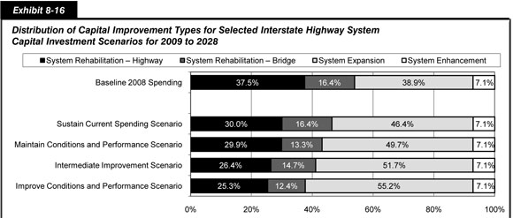
Scenario Name	Average Annual Investment (Billions of 2008 Dollars)
Scenario Name	System Rehabilitation Highway¹	System Rehabilitation Bridge²	System Rehabilitation Total	System Expansion ³	System Enhancement	Total
Baseline 2008 Spending	$7.5	$3.3	$10.8	$7.8	$1.4	$20.0
Sustain Current Spending scenario	$6.0	$3.3	$9.3	$9.3	$1.4	$20.0
Maintain Conditions and Performance scenario	$7.2	$3.2	$10.5	$12.0	$1.7	$24.3
Intermediate Improvement scenario	$9.6	$5.3	$14.9	$18.7	$2.6	$36.2
Improve Conditions and Performance scenario	$10.9	$5.3	$16.2	$23.7	$3.1	$43.0
State of Good Repair benchmark⁴	$10.9	$5.3	$16.2

¹ Values shown correspond to amounts in Exhibit 7-15 in Chapter 7.
² Values shown correspond to amounts in Exhibit 7-20 in Chapter 7.
³ Values shown correspond to amounts in Exhibit 7-16 in Chapter 7.
⁴ The State of Good Repair benchmark is a subset of the Improve Conditions and Performance scenario.

Sources: Highway Economic Requirements System and National Bridge Investment Analysis System.

Selected Transit Capital Investment Scenarios

While Chapter 7 considered the impacts of varying levels of capital investment on transit conditions and performance, this chapter provides in-depth analysis of four specific investment scenarios, as outlined below in Exhibit 8-17. The Sustain Current Spending scenario assesses the impact of sustaining current expenditure levels on asset conditions and system performance over the next 20-year period. Given that current expenditure rates are generally less than are required to maintain current condition and performance levels, this scenario generally reflects the magnitude of the expected declines in conditions and performance given maintenance of current capital investment rates. The State of Good Repair (SGR) benchmark considers the level of investment required to eliminate the existing capital investment backlog as well as the condition and performance impacts of doing so. In contrast to the other scenarios considered here, the SGR benchmark only considers the preservation needs of existing transit assets (with no consideration of expansion requirements). Moreover, this is the only scenario that does not require that investments pass the Transit Economic Requirements Model’s (TERM’s) benefit-cost test (hence, this scenario brings all assets to SGR regardless of TERM’s assessment of whether reinvestment is warranted). Finally, the Low Growth and High Growth scenarios both assess the required levels of reinvestment to (1) preserve existing transit assets at a condition rating of 2.50 or higher and (2) expand transit service capacity to support differing levels of ridership growth while passing TERM’s benefit-cost test.

Exhibit 8-17
2010 C&P Analysis Scenarios for Transit
Scenario Aspect	Sustain Current Spending	SGR	Low Growth (MPO Projected Growth)	High Growth (Historical Growth)
Description	Sustain preservation and expansion spending at current levels over next 20 years	Level of investment to attain and maintain SGR over next 20 years (no assessment of expansion needs)	Preserve existing assets and expand asset base to support MPO projected ridership growth (about 1.4%)	Preserve existing assets and expand asset base to support historical rate of ridership growth (2.8% between 1999 and 2008)
Objective	Assess impact of constrained funding on condition, SGR backlog and ridership capacity	Requirements to attain SGR (as defined by assets in condition 2.5 or better)	Assess unconstrained preservation and capacity expansion needs assuming low ridership growth	Assess unconstrained preservation and capacity expansion needs assuming high ridership growth
Apply Benefit-Cost Test?	Yes¹	No	Yes	Yes
Preservation?	Yes²	Yes ²	Yes ²	Yes ²
Expansion?	Yes	No	Yes	Yes

¹ To prioritize investments under constrained funding.
² Replace at condition 2.5.

Exhibit 8-18 summarizes the analysis results for each of these scenarios. It should be noted that each of the scenarios presented in Exhibit 8-18 imposes the same asset condition replacement threshold (i.e., assets are replaced at condition 2.50 when there is sufficient budget to do so) when assessing transit reinvestment needs. Hence, the differences in the total preservation expenditure amounts across each of these scenarios primarily reflect the impact of either (1) an imposed budget constraint (Sustain Current Spending scenario) or (2) application of TERM’s benefit-cost test (the SGR benchmark does not apply the benefit-cost test). A brief review of Exhibit 8-18 reveals the following:

Exhibit 8-18
Annual Average Cost by Investment Scenario (2008–2028)
Mode, Purpose, and Asset Type	Investment Projection (Billions of 2008 Dollars)
Mode, Purpose, and Asset Type	Sustain Current Spending	SGR	Low Growth	High Growth
Urbanized Areas Over 1 Million in Population¹
Nonrail ²
Preservation	$3.7	$4.9	$4.5	$4.6
Expansion	$1.0	$0.0	$1.1	$2.3
Subtotal Nonrail ³	$4.7	$4.9	$5.6	$6.9
Rail
Preservation	$6.5	$10.7	$10.0	$10.5
Expansion	$3.6	$0.0	$2.6	$4.4
Subtotal Rail ³	$10.1	$10.7	$12.7	$14.8
Total, Over 1 Million in Population ³	$14.8	$15.6	$18.2	$21.7
Urbanized Areas Under 1 Million in Population and Rural
Nonrail ²
Preservation	$0.8	$2.1	$1.9	$1.9
Expansion	$0.5	$0.0	$0.5	$0.7
Subtotal Nonrail ³	$1.3	$2.1	$2.4	$2.6
Rail
Preservation	$0.0	$0.3	$0.2	$0.2
Expansion	$0.0	$0.0	$0.0	$0.0
Subtotal Rail ³	$0.0	$0.3	$0.2	$0.2
Total, Under 1 Million and Rural ³	$1.3	$2.4	$2.5	$2.8
Total ³	$16.1	$18.0	$20.8	$24.5

¹ Includes 37 different UZAs.
² Buses, vans, and other (including ferryboats).
³ Note that totals may not sum due to rounding.

Source: Transit Economic Requirements Model.

Sustain Current Spending Scenario: Total spending under this scenario is well below that of each of the other needs—based scenarios, indicating that a sustainment of recent spending levels is insufficient to attain the investment objectives of the SGR, Low Growth, or High Growth scenarios (suggesting future increases in the size of the SGR backlog and a likely increase in the number of transit riders per peak vehicle—including an increased incidence of crowding—in the absence of increased levels of expenditures).
SGR Benchmark: The level of expenditures required to attain and maintain SGR over the upcoming 20-year period—which covers preservation needs but excludes any expenditures on expansion investments—is roughly 12 percent higher than that currently expended on asset preservation and expansion combined.
Low and High Growth Scenarios: The level of investment to address expected preservation and expansion needs is estimated to be roughly 33 percent to 55 percent higher than currently expended by the Nation’s transit operators. Preservation and expansion needs are highest for urbanized areas (UZAs) exceeding 1 million in population.

The following subsections present more detailed assessments of each scenario.

Sustain Current Spending Scenario

In 2008, as reported by transit agencies to the National Transit Database (NTD), transit operators spent a total of $16.1 billion on capital projects (see Exhibit 7-21 and the corresponding discussion in Chapter 7). Of this amount, $11.0 billion was dedicated to the preservation of existing assets while the remaining $5.1 billion was dedicated to investment in asset expansion both to support ongoing ridership growth and to improve service performance. This Sustain Current Spending scenario considers the expected impact on the long-term physical conditions and service performance of the Nation’s transit infrastructure if these 2008 expenditure levels are sustained in constant dollar terms through 2028. Similar to the discussion in Chapter 7, the analysis considers the impacts of asset preservation investments separately from those of asset expansion.

Capital Expenditures for 2008. It is important to note that the level of transit capital expenditures as reported to the NTD was higher in 2008 than at any other point in the 5-year period from 2004 through 2008 (see Exhibit 8-19). Even when adjusted for inflation, which was significant for capital assets over this period, total expenditures in 2008 were roughly $0.5 billion higher for preservation and $1.3 billion higher for expansion as compared with the average for the preceding 4-year period. Moreover, based on preliminary data for 2009, it is likely that this is a one-time, permanent increase in the reported level of transit capital expenditures (at least partially driven by changes in transit agency accounting practices).

Exhibit 8-19
Annual Transit Capital Expenditures, 2004 to 2008 (Billions of YOE Dollars)
Year	Preservation	Expansion	Total
2004	$9.40	$3.20	$12.60
2005	$9.00	$2.90	$11.80
2006	$9.30	$3.50	$12.80
2007	$9.60	$4.00	$13.60
2008	$11.00	$5.10	$16.10
Average	$9.70	$3.70	$13.40
Expenditures 2004 to 2007 in 2008 Dollars
Average	$10.50	$3.80	$14.70

Source: NTD.

Given that financial data is typically reported under the accrual basis of accounting, expenditures may be reported during periods when costs are accrued, not when they are paid. If an operator changes accounting practices for employee expenses (e.g., salaries, wages, benefits, etc.), for example, financial trends may show an increase or decrease from one accounting period to another that would not otherwise have appeared.

In 2004, the Governmental Accounting Standard Board issued a statement (Statement No. 45) regarding the accounting for post-employment benefits. Examples of these benefits include healthcare and life insurance (the statement does not address accounting for pensions). This statement, which was phased in over three years starting with accounting periods after 2006, now requires the accrued costs of these benefits to be accounted for during the employee’s period of employment as opposed to when they are paid. For state and local governmental employers that apply this accounting approach, their financial data and trends—including changes in total reported expenditures—may reflect changes that otherwise would not have been reported, all else being equal. This may account for the significant increases in expenses and funding reported to NTD as of 2008. Hence, it should be noted that the 2008 level of transit capital expenditures is expected to be representative of future years’ levels.

TERM’s Funding Allocation. The following analysis of the Sustain Current Spending scenario relies on TERM’s allocation of 2008-level preservation and expansion expenditures to the Nation’s existing transit operators, their modes, and their assets over the upcoming 20-year period as depicted in Exhibit 8-20. As with other TERM analyses involving the allocation of constrained transit funds, TERM allocates limited funds based on the results of the model’s benefit-cost analysis, which ranks potential investments based on their assessed benefit-cost ratios (with the highest-ranked investments being funded first). Note that this TERM benefit-cost–based allocation of funding between assets and modes may differ from the allocation that local agencies might actually pursue assuming total spending is sustained at current levels over 20 years.

Exhibit 8-20
Sustain Current Spending Scenario: Average Annual Investment by Asset Type, 2008–2028 (Billions of 2008 Dollars)
Asset Type	Investment Category		Total
Asset Type	Preservation	Expansion	Total
Rail
Guideway Elements	$1.4	$1.0	$2.4
Facilities	$0.6	$0.1	$0.6
Systems	$2.4	$0.2	$2.6
Stations	$1.0	$0.6	$1.6
Vehicles	$1.1	$0.8	$2.0
Other Project Costs		$0.9	$0.9
Subtotal Rail^*	$6.5	$3.6	$10.1
Nonrail
Guideway Elements	$0.4	$0.1	$0.5
Facilities	$0.8	$0.3	$1.0
Systems	$0.0	$0.0	$0.1
Stations	$0.0	$0.0	$0.1
Vehicles	$3.2	$1.1	$4.3
Other Project Costs		$0.0	$0.0
Subtotal Nonrail*	$4.5	$1.5	$6.0
Total*	$11.0	$5.1	$16.1

^* Note that totals may not sum due to rounding.

Source: Transit Economic Requirements Model and FTA staff estimates.

Preservation Investments

As noted above, transit operators spent an estimated $11.0 billion in 2008 on the rehabilitation and replacement of existing transit infrastructure. Based on current TERM analysis, this level of reinvestment is less than that required to address the anticipated reinvestment needs of the Nation’s existing transit assets, and, if sustained over the forecasted 20-year period, would result in an overall decline in the condition of existing transit assets as well as an increase in the size of the investment backlog.

For example, Exhibit 8-21 presents the projected increase in the proportion of existing assets that exceed their useful life, by asset category, over the period 2008 to 2028. Given the benefit-cost–based prioritization imposed by TERM for this scenario, the proportion of existing assets that exceed their useful life is projected to undergo a near-continuous increase across each of these asset categories. (This condition projection uses TERM’s benefit-cost test to prioritize rehabilitation and replacement investments in this scenario. Specifically, for each investment period in the forecast, TERM ranks all proposed investment activities based on their assessed benefit-cost ratios [highest to lowest]. TERM then invests in the highest-ranked projects for each period until the available funding for the period is exhausted. Investments not addressed in the current period as a result of the funding constraint are then deferred until the following period.) Also, given that the proportion of “over-age” assets is projected to increase for all asset categories under this prioritization, it is clear that any reprioritization to favor reinvestment in one asset category over another would only serve to accelerate the rate of increase of the remaining categories. Note that these over-age assets tend to deliver the lowest-quality transit service to system users (e.g., have the highest likelihood of in-service failures).

Exhibit 8-21. Sustain Current Spending Scenario: Over-Age Forecast by Asset Category, 2008-2028. Line chart with markers showing the percentages of assets exceeding their useful life by value and by forecast year for five asset categories from 2008 to 2028. The trends in this line chart are generally upward. The share of guideway elements projected to exceed their useful value will rise from 16.9 percent in 2008 to 29.3 percent in 2028. The share of facilities projected to exceed their useful value will rise from 14.2 percent in 2008 to 34.1 percent in 2028. The share of systems projected to exceed their useful value will rise from 23.5 percent in 2008 to 33.6 percent in 2028. The share of stations projected to exceed their useful value will rise from 15.6 percent in 2008 to 26.2 percent in 2028. The share of vehicles projected to exceed their useful value equaled 16.2 percent in 2008, will spike to 35.4 percent in 2019, and will fall to 29.3 percent in 2028. Note that the proportion of assets exceeding their useful life is measured based on asset replacement value, not asset quantities. Source: Transit Economic Requirements Model.

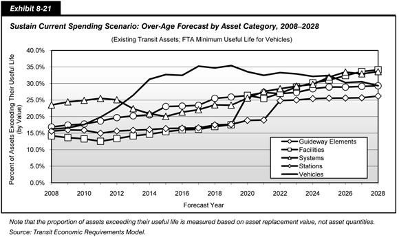
Finally, Exhibit 8-22 presents the projected change in the size of the investment backlog if reinvestment levels are sustained at the 2008 level of $11.0 billion, in constant dollar terms. As described in Chapter 7, the investment backlog represents the level of investment required to replace all assets that exceed their useful life and also to address all rehabilitation activities that are currently past due. Given that the current rate of capital reinvestment is insufficient to address the replacement needs of the existing stock of transit assets, the size of that backlog is projected to increase from the currently estimated level of $78 billion to roughly $116 billion by 2028. This chart also divides the backlog amount according to transit service area size, with the lower portion showing the backlog for UZAs with populations greater than 1 million and the upper portion showing the backlog for all other UZAs and rural areas combined. This segmentation highlights the significantly higher existing backlog for those UZAs serving the largest number of transit riders. The initial reduction in the backlog for these largest-transit UZAs, as shown in Exhibit 8-22, results from TERM’s higher prioritization of replacement needs for this urban area type and does not necessarily reflect the actual or expected allocation of expenditures between urban area types given maintenance of current spending levels in the future. Regardless of the actual allocation, it is clear that the 2008 expenditure level of $11.0 billion, if sustained, is not sufficient to prevent a further increase in the backlog needs of one or more of these UZA types.

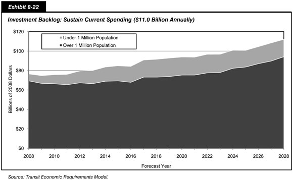
Exhibit 8-22. Investment Backlog: Sustain Current Spending ($11.0 Billion Annually). Stacked area chart showing projected changes in the investment backlog in areas over 1 million and under 1 million in population when investment is sustained at the current spending level of 11.0 billion dollars annually in 2008 dollars. In 2008, the investment backlog was 69.4 billion dollars in areas over 1 million in population and is projected to rise to 94.3 billion dollars in 2028. In 2008, the investment backlog was 7.2 billion dollars in areas under 1 million in population and is projected to rise to 17.8 billion dollars in 2028. Source: Transit Economic Requirements Model.

Expansion Investments

In addition to the $11.0 billion spent on transit asset preservation in 2008, transit agencies spent $5.1 billion on expansion investments to support ridership growth and to improve transit performance. This section considers the impact of sustaining the 2008 level of expansion investment on future ridership capacity and vehicle utilization rates under both lower and higher ridership growth rate assumptions. As noted above, it is important to consider here that the $5.1 billion spent on expansion investments in 2008 was significantly higher than that reported in prior years.

As already considered in Chapter 7 (see Exhibit 7-27), the 2008 rate of investment in transit expansion is not sufficient to expand transit capacity at a rate equal to the rate of growth in travel demand, as projected by the Nation’s Metropolitan Planning Organizations (MPOs) or based on the historical trend rate of increase. Under these circumstances, it should be expected that transit capacity utilization (e.g., passengers per vehicle) will increase, with the level of increase determined by actual growth in demand. Although the impact of this change may be minimal for systems that currently have lower capacity utilization, service performance on some higher utilization systems would likely decline as riders experience increased vehicle crowding and potential for service delays. This impact is illustrated in Exhibit 8-23, which presents the projected change in vehicle occupancy rates by mode during the period from 2008 through 2028 (reflecting the impacts of spending from 2009 through 2028) under both lower (MPO) and higher (trend) rates of growth in transit scenarios, assuming that transit agencies continue to invest an average of $5.1 billion per year on transit expansion. Under both the MPO projected and the historical trend rates of increase, there is a steady rise in the average number of riders per transit vehicle across each of the four modes depicted here, with the impact being small under the MPO projected rate of growth but significant under the trend rate of growth scenario, which is higher. For perspective, note that MPO growth rate projections tend to be conservative because they are developed based on financially constrained transportation plans. Moreover, the actual growth in travel demand has typically exceeded the MPO growth projections for much of the past decade.

Exhibit 8-23. Sustain Current Spending Scenario: Capacity Utilization by Mode Forecast, 2008-2028. Line chart with markers showing changes in average vehicle occupancy for four vehicle modes projected by metropolitan planning organizations and by growth trends from 2008 to 2028. For motor buses, average vehicle occupancy is projected to rise from 10.84 in 2008 to 11.31 by the metropolitan planning organizations and to 14.50 by growth trend. For light rail, average vehicle occupancy is projected to rise from 24.10 in 2008 to 25.43 by the metropolitan planning organizations and to 30.22 by growth trend. For heavy rail, average vehicle occupancy is projected to rise from 25.71 in 2008 to 26.46 by the metropolitan planning organizations and to 35.88 by growth trend. For commuter rail, average vehicle occupancy is projected to rise from 35.70 in 2008 to 36.60 by the metropolitan planning organizations and to 49.69 by growth trend. Source: Transit Economic Requirements Model.

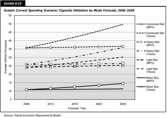
Exhibit 8-24 presents the projected growth in transit riders that can be supported by the 2008 level of investment (keeping vehicle occupancy rates constant) as compared with the potential growth in total ridership under both the low- and higher-growth rate scenarios. Similar to prior analyses, the $5.1-billion level of investment can support ridership growth that is similar to the MPO projected ridership increases, but is short of that required to support continued ridership growth at recent historical rates (i.e., without impacting service performance).

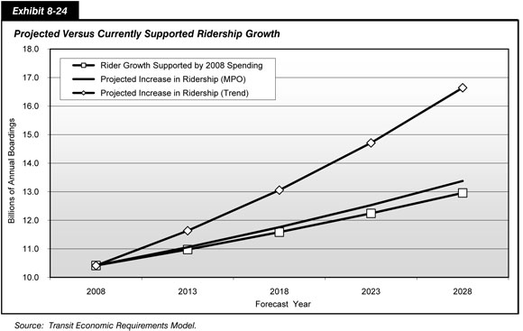
Exhibit 8-24. Projected Versus Currently Supported Ridership Growth. Line chart with markers showing increases in annual passenger boardings in billions as supported by 2008 spending, as projected by metropolitan planning organizations, and as projected by the growth trend from 2008 to 2028. From the 2008 level of 10.3 billion, 2008 spending supported 13.0 billion annual boardings, metropolitan planning organizations projected an increase to 13.4 billion, and the growth trend projected an increase to 16.6 billion. Source: Transit Economic Requirements Model.

State of Good Repair Benchmark

The preceding scenario considered the impacts of sustaining transit spending at current levels, which appear to be insufficient to address either deferred investment needs (which are projected to increase) or the projected increases in transit ridership (without a reduction in service performance). In contrast, this section focuses on the level of investment required both to eliminate the investment backlog over the next 20 years and to provide for sustainable rehabilitation and replacement needs once the backlog has been addressed. Specifically, the SGR benchmark estimates the level of annual investment required to replace assets that currently exceed their useful life, to address all deferred rehabilitation activities (yielding a state of good repair where the asset has a condition rating of 2.50 or higher), and then to address all future rehabilitation and replacement activities as they come due. The SGR benchmark considered here is the same as that described in the Federal Transit Administration’s National State of Good Repair study, released July 2010.

What is the definition of a State of Good Repair for transit assets?
The definition of “state of good repair” used for this scenario relies on TERM's assessment of transit asset conditions. Specifically, for this scenario, TERM considers assets to be in a state of good repair if they are rated at condition rating of 2.50 or higher and if all required rehabilitation activities have been addressed.

Differences with Other Scenarios: In contrast to the other scenarios in this Chapter, the SGR benchmark (1) makes no assessment of expansion needs and (2) does not apply TERM’s benefit-cost test to investments proposed by TERM. These benchmark characteristics are considered consistent with the concept of “state of good repair.” First, analyses of expansion investments are ultimately focused on capacity improvements and not on the needs of deteriorated assets. Second, application of TERM’s benefit-cost test would leave some reinvestment needs unaddressed. The intention of this benchmark is to assess the total magnitude of unaddressed reinvestment needs for all transit assets currently in service, regardless of whether it appears to be cost-beneficial for these assets to remain in service.

SGR Investment Needs

Annual reinvestment needs under the SGR benchmark are presented in Exhibit 8-25. Under this benchmark, an estimated $18.0 billion in annual expenditures is required over the next 20 years to bring the condition of all existing transit assets to an SGR. Of this amount, roughly $11.0 billion (60 percent) is required to address the SGR needs of rail assets. Note that a large proportion of rail reinvestment needs are associated with guideway elements (primarily aging elevated and tunnel structures) and rail systems (including train control, traction power, and communications systems) that are past their useful life and potentially technologically obsolete as well. Bus-related reinvestment needs are primarily associated with aging vehicle fleets.

Exhibit 8-25
SGR Benchmark: Average Annual Investment by Asset Type, 2008–2028 (Billions of 2008 Dollars)
Asset Type	Urban Area Type		Total
Asset Type	Over 1 Million Population	Under 1 Million Population	Total
Rail
Guideway Elements	$2.9	$0.1	$3.0
Facilities	$1.1	$0.1	$1.1
Systems	$3.2	$0.0	$3.2
Stations	$1.8	$0.0	$1.8
Vehicles	$1.8	$0.0	$1.8
Subtotal Rail^*	$10.7	$0.3	$11.0
Nonrail
Guideway Elements	$0.4	$0.1	$0.5
Facilities	$1.1	$0.7	$1.7
Systems	$0.1	$0.0	$0.2
Stations	$0.1	$0.0	$0.1
Vehicles	$3.2	$1.3	$4.6
Subtotal Nonrail*	$4.9	$2.1	$7.0
Total*	$15.6	$2.4	$18.0

^* Note that totals may not sum due to rounding.

Source: Transit Economic Requirements Model.

Exhibit 8-25 also provides a breakout of capital reinvestment needs by type of UZA. This breakout emphasizes the fact that capital reinvestment needs are most heavily concentrated in the Nation’s larger UZAs. Together, these urban areas account for close to 87 percent of total reinvestment needs (across all mode and asset types), with the rail reinvestment needs of these urban areas accounting for more than one-half of the total reinvestment required to bring all assets to an SGR. This high proportion of total needs reflects the high level of investment in older assets found in these urban areas.

Impact on the Investment Backlog

A key objective of the SGR benchmark is to determine the level of investment required to attain and then maintain an SGR across all transit assets over the next 20 years, including elimination of the existing investment backlog. Exhibit 8-26 shows the estimated impact of the $18.0 billion in annual expenditures under the SGR benchmark on the existing investment backlog over the 20-year forecast period (compare these data with Exhibit 8-22). Given this level of expenditures, the backlog is projected to be eliminated by 2028, with the majority of this drawdown addressing the reinvestment needs of the UZAs with populations greater than 1 million.

Exhibit 8-26. Investment Backlog: SGR Benchmark ($18.0 Billion Annually). Stacked area chart showing projected changes in the investment backlog in areas over 1 million and under 1 million in population when investment is raised to the state-of-good-repair benchmark level of 18.0 billion dollars annually in 2008 dollars. In 2008, the investment backlog was 69.4 billion dollars in areas over 1 million in population and is projected to be eliminated by 2028. In 2008, the investment backlog was 7.2 billion dollars in areas under 1 million in population and is projected to be eliminated by 2028. Source: Transit Economic Requirements Model.

Impact on Conditions

In drawing down the investment backlog, the annual capital expenditures of $18.0 billion under the SGR benchmark would also lead to the replacement of assets with an estimated condition rating of 2.5 or lower. Within TERM’s condition rating system, this includes assets in marginal condition that have ratings of below 2.5 and all assets in poor condition. Exhibit 8-27 shows the current distribution of asset conditions for assets estimated to be in a rating condition of 2.50 or lower (with assets in poor condition segmented into two sub-groups). Note that this graphic excludes both tunnel structures and subway stations in tunnel structures because these are considered assets that require ongoing capital rehabilitation expenditures but that are never actually replaced. As with the investment backlog, the proportion of assets at rating condition 2.50 or lower is projected to decrease under the SGR benchmark from roughly 10 percent of assets in 2008 to well below 1 percent by 2028. Once again, this replacement activity would remove from service those assets with higher occurrences of service failures, technological obsolescence, and lower overall service quality.

Exhibit 8-27. Proportion of Transit Assets Not in SGR (Excluding Tunnel Structures). Stacked area chart showing percentage of all transit assets by value estimated by three condition rating from 2008 to 2028. In 2008, the share of transit assets in poor condition of 1.0 to 1.5 equaled 3.92 percent, the share in poor condition of 1.5 to 2.0 equaled 1.61 percent, and the share in marginal condition of 2.0 to 2.5 equaled 5.14 percent. By 2028, the share of transit assets in poor or marginal condition is projected to be negligible. Source: Transit Economic Requirements Model.

Impact on Vehicle Fleet Performance

While the preceding analysis has considered the impact of higher investment on reducing the investment backlog and potential replacement of assets past their useful life, this analysis may not provide a sense of the potential positive implications of these changes for daily transit service. To help better understand these effects, Exhibit 8-28 shows the estimated percent reduction in fleet-wide revenue service disruptions (relative to 2008) for heavy rail and motor bus vehicles resulting from the retirement of over-age transit passenger vehicles under the SGR benchmark. Note that the large variation in the percent reduction for bus is a result of the timing of large bus fleet replacements. Also, while the reductions in service disruptions is significant for bus and heavy rail vehicles, some vehicle types (e.g., light and commuter rail) actually show a net increase in service disruptions under the SGR benchmark; this is because the current age distribution for these fleets is skewed toward younger vehicle ages and is not sustainable in the longer term. This effect is the result of the recent development of new light rail and commuter rail systems.

Exhibit 8-28. Percent Reduction in Revenue Service Disruptions Relative to 2008 for SGR Benchmark. Line chart showing percentages of reductions in revenue service disruptions estimated for heavy rail and motor bus from 2008 to 2028. The trend in this line chart is downward. The share of heavy rail revenue service disruptions is estimated at minus19 percent in 2028. The share of motor bus revenue service disruptions is estimated at minus 19 percent in 2013, minus 12 percent in 2023, and minus 18 percent in 2028. Source: Transit Economic Requirements Model.

Low and High Growth Scenarios

The preceding scenario considered the level of investment to bring existing transit assets to a SGR but in doing so did not consider either (1) the cost effectiveness of these investments (investments were not required to pass TERM’s benefit-cost test) or (2) the level of expansion investment required to support projected ridership growth. The Low Growth scenario and High Growth scenario address both of these issues. Specifically, these scenarios use the same rules to assess when assets should be rehabilitated or replaced as were applied in the preceding SGR benchmark (e.g., with assets being replaced at condition 2.50), but also require that these preservation and expansion investments pass TERM’s benefit-cost test. In general, some reinvestment activities do not pass this test (i.e., have a benefit-cost ratio of less than one), which can result from low ridership benefits, higher capital or operating costs, or a mix of these factors. Excluding investments that do not pass the benefit-cost test has the effect of reducing total estimated needs.

In addition, the Low and High Growth scenarios also assess transit expansion needs given ridership growth as projected by the Nation’s MPOs (low growth) and based on the average annual compound rate as experienced over the last 10-year period (high growth). For the expansion component of this scenario, TERM assesses the level of investment required to maintain current vehicle occupancy rates (at the agency-mode level) subject to the rate of projected growth in transit demand in that UZA and also subject to the proposed expansion investment passing TERM’s benefit-cost test.

Low Growth Assumption

The Low Growth scenario is intended to provide a lower bound on the level of investment required to maintain current service performance (as measured by transit vehicle capacity utilization) as determined by a relatively low rate of growth in travel demand. In particular, this Low Growth scenario relies on growth in travel demand as projected by a sample of the MPOs (representing the Nation’s 30 largest UZAs and a sample of smaller UZAs). When aggregated across the Nation’s UZAs (and corrected for differences in transit demand by UZA), this source yields a national average annual growth rate of 1.4 percent over the 20-year period from 2008 to 2028. (This represents the weighted average growth rate at the national level. In practice, the ridership growth rates applied by TERM vary by UZA based on the growth projections obtained from that UZA’s MPO.)

The MPO projections are considered low (or at least conservative) for the following reasons. First, MPO transit demand projections are financially constrained (i.e., projected ridership growth is limited by the expected capacity to fund expansion projects) and, hence, these projections are lower than the potential for increased ridership demand if funding were unconstrained. Second, as discussed further in Chapter 9, the historical rate of increase in transit ridership and transit passenger miles have generally exceeded MPO growth projections for these same time periods, again tending to characterize the MPO growth projections as relatively low or conservative.

High Growth Assumption

Similarly, the High Growth scenario provides a higher bound on the level of investment required to maintain current service performance as determined by a relatively high rate of growth in travel demand. In particular, the High Growth scenario relies on the trend rate of growth in transit passenger miles over the period 1999 through 2008 as reported to the NTD. When calculated across all transit operators, this historical trend rate of growth converts to a national average compound annual growth rate of 2.78 percent during this time period. Similar to the MPO growth rates in the Low Growth scenario, the 10-year trend growth rates applied by TERM for the High Growth scenario also vary by UZA either based on the actual trend rates of growth experienced by each UZA (for UZAs close to or higher than 1 million in population) or based on the average for UZAs of comparable size in the same geographic region.

This rate is considered relatively high primarily due to the unusually high rate of growth in ridership experienced over the period from roughly 2006 to 2008, partly in response to high fuel prices. The growth rate for this High Growth scenario is very close to double that of the Low Growth scenario.

Low and High Growth Scenario Needs

TERM’s projected annual average capital investment needs under the Low and High Growth scenarios—including those for both asset preservation and asset expansion—is presented in Exhibit 8-29.

Exhibit 8-29
Low and High Growth Scenarios: Average Annual Investment by Asset Type, 2008–2028 (Billions of 2008 Dollars)
Asset Type	Lower Growth (MPO; 1.4%)		Total	Higher Growth (10-Year Trend; 2.8%)		Total
Asset Type	Preservation	Expansion	Total	Preservation	Expansion	Total
Rail
Guideway Elements	$2.7	$0.7	$3.4	$2.9	$0.8	$3.7
Facilities	$1.0	$0.1	$1.1	$1.0	$0.2	$1.2
Systems	$3.1	$0.2	$3.3	$3.2	$0.2	$3.4
Stations	$1.6	$0.4	$2.0	$1.8	$0.5	$2.3
Vehicles	$1.8	$0.7	$2.4	$1.8	$1.9	$3.7
Other Project Costs	$0.0	$0.7	$0.7	$0.0	$0.8	$0.8
Subtotal Rail^*	$10.2	$2.6	$12.8	$10.7	$4.4	$15.0
Nonrail
Guideway Elements	$0.4	$0.1	$0.5	$0.5	$0.1	$0.5
Facilities	$1.4	$0.3	$1.7	$1.5	$0.6	$2.0
Systems	$0.1	$0.0	$0.2	$0.1	$0.0	$0.2
Stations	$0.0	$0.0	$0.1	$0.0	$0.0	$0.1
Vehicles	$4.3	$1.2	$5.5	$4.4	$2.2	$6.6
Other Project Costs	$0.0	$0.0	$0.0	$0.0	$0.0	$0.0
Subtotal Nonrail*	$6.3	$1.6	$7.9	$6.5	$2.9	$9.4
Total Investment*	$16.6	$4.2	$20.8	$17.2	$7.3	$24.5

^* Note that totals may not sum due to rounding.

Source: Transit Economic Requirements Model.

Lower Growth Needs

Assuming the relatively low ridership growth in the Low Growth scenario, total investment needs for both system preservation and expansion are estimated to average roughly $20.8 billion each year for the next two decades. Of this amount, roughly 80 percent are for preservation of existing assets and close to half is associated with preservation of existing rail infrastructure alone. Note that the $1.4 billion difference between the $18.0 billion in annual preservation needs under the SGR benchmark and the $16.6 billion in preservation needs under the Low Growth scenario is entirely due to the application of TERM’s benefit-cost test under the Low Growth scenario. Finally, expansion needs in this scenario total $4.2 billion annually, with more than half of that amount associated with rail expansion costs.

Higher Growth Needs

In contrast, total investment needs under the High Growth scenario are estimated to be $24.5 billion annually. This includes $17.2 billion for system preservation and an additional $7.3 billion for system expansion. Note that system preservation costs are higher under the High Growth scenario because the higher growth rate leads to a larger expansion of the asset base as compared to the Low Growth scenario. Under this scenario, investment in rail assets is still larger than that for bus expansion but both rail and non-rail continue to have roughly equal shares of the expansion total (60 percent for rail and 40 percent for non-rail). However, at the asset category level, investment requirements for additional fleet capacity appear to be greater under the High Growth scenario (increasing from roughly 45 percent of expansion needs under the Low Growth scenario to just under 60 percent in the High Growth scenario). Overall, total expansion investment needs are roughly 70 percent higher for the High Growth scenario than for the Low Growth scenario (despite an approximate doubling in the overall growth rate).

Impact on Conditions and Performance

The impact of the Low and High Growth Rate preservation investments on transit conditions is essentially the same as that already presented for the SGR benchmark in Exhibit 8-26 and Exhibit 8-27. As noted above, these scenarios use the same rules to assess when assets should be rehabilitated or replaced as were applied in the SGR benchmark (e.g., with assets being replaced at condition rating 2.50). In terms of asset conditions, the primary difference between the SGR benchmark and the Low and High Growth scenarios relates to: (1) TERM’s benefit-cost test not applying to the SGR benchmark (leading to higher SGR preservation needs overall) and (2) the Low and High Growth scenarios having some additional needs for the replacement of expansion assets with short service lives. Together, these impacts tend to work in opposite directions with the result that the rate of drawdown in the investment backlog and the elimination of assets exceeding their useful life are roughly comparable for each of these three scenarios.

Similarly, the impact of the Low and High Growth rate expansion investments on transit performance was considered in Exhibit 8-24. That analysis demonstrated the significant difference in the level of ridership growth supported by the High Growth scenario as compared with either the current level of expenditures ($5.1 billion in 2008) or the rate of growth supported under the Low Growth scenario.

Scenario Benefits Comparison

Finally, this subsection summarizes and compares many of the investment benefits associated with each of the four analysis scenarios considered above. While much of this comparison is based on measures already introduced above, this discussion also considers a few additional investment impact measures. These comparisons are presented in Exhibit 8-30. Note that the first column of data in Exhibit 8-30 presents the current values for each of these measures (as of 2008). The subsequent columns present the estimated future values in 2028 assuming the levels, allocations, and timing of expenditures associated with each of the four investment scenarios.

Exhibit 8-30
Scenario Investment Benefits Scorecard
Measure	Baseline 2008 Actual Spending, Conditions and Performance	Scenarios for 2028
Measure	Baseline 2008 Actual Spending, Conditions and Performance	Sustain Current Spending	SGR	Low Growth	High Growth
Average Annual Expenditures (Billions of 2008 Dollars)
Preservation	$11.0	$11.0	$18.0	$16.6	$17.2
Expansion	$5.1	$5.1	na	$4.2	$7.3
Total	$16.1	$16.1	$18.0	$20.8	$24.5
Conditions (Existing Assets)
Average Physical Condition Rating	3.78	3.38	3.59	3.57	3.58
Investment Backlog (Billions of Dollars)	$77.7	$112.5	$0.0	$0.0	$0.0
Investment Backlog (% of Replacement Costs)	11.7%	17.0%	0.0%	0.0%	0.0%
Backlog Ratio¹	5.4	7.8	0.0	0.0	0.0
Performance
Ridership Impacts of Expansion Investments (2028)
New Boardings Supported by Expansion (Billions)	na	2.5	na	2.6	6.2
CO ₂ Emissions Avoided (Millions of Metric Tons)	na	1.6	na	1.7	4.0
Fleet Performance
Revenue Service Disruptions per PMT	9.6	10.5	8.6	8.6	8.6
Fleet Maintenance Cost per Revenue Vehicle Mile	$1.70	$1.76	$1.59	$1.59	$1.59
Other Benefits
Job Years Impact (Thousands)²
Operating and Maintenance	1,201.7	1,554.5	1,201.7	1,590.8	1,945.1
Capital	257.6	257.6	288.0	332.8	392.0
Total Annual Job Years Supported	1,459.3	1,812.1	1,489.7	1,923.6	2,337.1
GDP Impact (Billions of Dollars)
Operating and Maintenance	$71.1	$92.0	$71.1	$94.1	$115.1
Capital	$21.5	$21.5	$24.0	$27.7	$32.7
Total Annual Incremental Impact	$92.6	$113.4	$95.1	$121.8	$147.7

¹ The backlog ratio is the ratio of the current investment backlog to the annual level of investment to maintain SGR once the backlog is eliminated.
² Includes direct, indirect, and induced impacts.

Exhibit 8-30 includes the following measures:

Average Annual Expenditures in billions of dollars: This amount is broken down into preservation and expansion expenditures.
Condition of Existing Assets: This analysis only considers the impact of investment funds on the condition of those assets currently in service.
Average Physical Condition Rating: The weighted average condition of all existing assets on TERM’s condition scale of 5 (excellent) through 1 (poor).

Investment Backlog: The value of all deferred capital investment, including assets exceeding their useful lives and rehabilitation activities that are past due (this value can approach but never reach zero due to assets continually aging with some exceeding their useful life). The backlog is presented here both as a total dollar amount and also as a percent of the total replacement value of all U.S. transit assets.

Backlog Ratio: The ratio of the current investment backlog to the annual level of investment required to maintain normal annual capital needs once the backlog is eliminated.
Performance Measures: The impact of investments on U.S. transit ridership capacity and system reliability.
New Boardings Supported by Expansion Investments: The number of additional riders that transit systems can carry without a loss in performance (given the projected ridership assumptions for each scenario).

Carbon Dioxide (CO₂) Emissions Avoided (millions of metric tons): Potential reduction in CO₂ emissions from providing the additional transit rider carrying capacity (assumes that riders would otherwise use other modes of travel, including automobiles).

Revenue Service Disruptions per Passenger Mile Travelled: Number of disruptions to revenue service per million passenger miles.

Fleet Maintenance Cost per Revenue Vehicle Mile: Fleet maintenance costs tend to increase with fleet age (or reduced asset condition). This measure estimates the change in fleet maintenance costs expressed in a per-revenue-vehicle-mile basis.
Other Benefits: Impacts other than those to transit conditions and performance. The jobs and Gross Domestic Product (GDP) impacts considered here were determined using an input-output analysis.
Jobs Impacts: The number of job years associated with both transit mode operations and ongoing capital investment (both preservation and expansion), including direct, indirect and induced job years. Each $1 million invested in transit operation activities is estimated to support 33 job years while each $1 million invested in transit capital investments supports 16 job years.

GDP Impacts: The impact on GDP associated with both transit mode operations and ongoing capital investment (both preservation and expansion), including direct, indirect and induced impacts. Each $1 invested in transit operation activities is estimated to generate $0.95 in additional GDP while each $1 invested in transit capital investments generates $0.33 in additional GDP.

Scorecard Comparisons

A review of the scorecard results for each of the four investment scenarios reveals the impacts discussed below.

Preservation Impacts

Continued reinvestment at the 2008 level is likely to yield a decline in overall asset conditions, an increase in the size of the investment backlog, and an increase in both service disruptions per million passenger miles and in maintenance costs per revenue vehicle mile. In contrast, with the exception of overall asset conditions, each of these measures is projected to improve under the SGR, Low Growth, and High Growth scenarios, each of which project roughly comparable levels of required capital reinvestment expenditures. Note that the overall condition rating measure of roughly 3.6 under these last three investment scenarios represents a sustainable, long-term condition level for the Nation’s existing transit assets over the long term (in contrast to the current measure of roughly 3.8, which would be difficult to maintain in the long term without replacing many asset types prior to the conclusion of their expected useful lives).

Expansion Impacts

While continued expansion investment at the 2008 level appears sufficient to support a relatively low rate of increase in transit ridership, recent historical rates of growth suggest that a significantly higher rate of expansion investment is required to avoid a decline in overall transit performance (e.g., in the form of increased crowding on high utilization systems). Higher rates of transit expansion investment, as required to support higher transit ridership growth or through a shift from auto travel to transit, can also help yield reductions in CO₂ emissions. Finally, higher rates of expansion investment also tend to support higher direct, indirect and induced impacts on jobs and other economic activity related to transit operations, construction, and rehabilitation activities.