FHWA > Policy > Transportation Investment: New Insights from Economic Analysis

Appendix B: A Preliminary Assessment of the Similarity Between Nadiri's s Industry Cost Elasticity and TSA's Transport Intensity Measure

Introduction

The U.S. Transportation Satellite Accounts (TSA) for 1992 were jointly developed by the Bureau of Transportation Statistics (BTS) of the U.S. Department of Transportation and the Bureau of Economic Analysis of the U.S. Department of Commerce. The primary purpose of this project was to address the under-representation of transportation activities in national economic accounts. The magnitude of transportation services has long been underestimated in national economic data used by government and private-sector decisionmakers. One reason is that, until now, national measures of transportation services only included the value of for-hire transportation, that is, transportation services provided by transportation firms to industries and the public on a for-hire basis. The sizable quantity of transportation activities performed by nontransportation industries, or in-house transportation, were not explicitly identified, and their output was counted as part of those nontransportation industries' output, rather than transportation output.

The publication of TSA 1992 in April 1998 provided, for the first time, much more complete and accurate estimates of transportation activities in the U.S. economy and their contributions to Gross Domestic Product. More important, the TSA 1992 provides this information on an industry basis. Detailed data on the use of transportation services at the industry level reveal several important features concerning the role of transportation in industry production, and transportation intensity coefficients from the TSA provide an empirical basis for productivity study.

Contribution of Highway Capital to Output and Productivity Growth in the U.S. Economy and Industries, by Nadiri and Manuneas, analyzed and measured the contribution of highway capital to private sector productivity growth. Using disaggregated data for 35 industry sectors, Nadiri's model identified the determinants of productivity growth for each industry, including the contribution of public highway capital. The cost elasticities with respect to highway capital for each of the 35 industry sector in Nadiri's study indicated that an increase in highway capital reduced cost in all but three industry sectors. There is a fairly wide range in the magnitudes of the cost elasticities across industries. Why is this so? Nadiri speculated that industries with large negative cost elasticities were probably intensive users of the highway network while industries with small cost elasticities were less intensive users. (See page 39 of Contribution of Highway Capital to Output and Productivity Growth in the U.S. Economy and Industries, Nadiri and Manuneas, 1998.)

The goal of this research note is to test Nadiri's speculation through correlation analysis of the cost elasticities with respect to highway capital reported in Nadiri's latest study and the transportation intensity coefficients from TSA 1992.

Match Industry Classification of TSA 1992 with that in Nadiri's Study

The first step of our analysis was to match industry classifications used in TSA 1992 with the 35 industry sectors used in Nadiri's study. In TSA 1992, the industry classification is much finer, consisting of about 500 industry classifications. Hence, the natural choice to bring the industries in the two projects to a comparable basis is to aggregate the 500 industries in TSA 1992 into the 35 industries. Since industry classifications in both Nadiri's study and TSA 1992 were based on Standard Industry Classification (SIC) codes, the aggregation was relatively straightforward.

Table 1 presents the 35 industry classifications used by Professor Nadiri, their average cost elasticities with respect to highway capital for the period 1981-1991, and their corresponding aggregated transportation intensities from TSA 1992.

Table 1: Nadiri's Cost Elasticity Estimates and TSA's Transportation Intensity Estimates by Industry Sector

Industry	1981–1991 average CE to highway infrastructures	Total transportation intensity coefficient	HW transportation intensity coefficient	Logistic cost per $ output (Proxy A)	Logistic cost per $ output (Proxy B)	Total intermediate inputs per $ output
1 Agriculture, forestry, fishery	-0.054	0.08	0.069	0.173	0.159	0.637
2 Metal mining	0.013	0.06	0.051	0.118	0.108	0.626
3 Coal mining	-1.279	0.089	0.052	0.148	0.111	0.445
4 Crude petroleum and natural gas	-0.041	0.021	0.016	0.220	0.214	0.542
5 Non metallic mineral mining	0.002	0.102	0.094	0.156	0.148	0.457
6 Construction	-0.073	0.077	6.976	0.190	0.186	0.584
7 Food and kindred products	-0.063	0.038	0.027	0.101	0.090	0.702
8 Tobacco manufacture products	-0.013	0.009	0.006	0.128	0.125	0.360
9 Textile mill products	-0.029	0.028	0.020	0.076	0.068	0.663
10 Apparel and other textile products	-0.031	0.021	0.017	0.104	0.099	0.657
11 Lumber and wood products	-0.031	0.048	0.036	0.100	0.088	0.642
12 Furniture and fixtures	-0.018	0.051	0.045	0.118	0.111	0.571
13 Paper and allied products	-0.041	0.052	0.036	0.108	0.091	0.622
14 Printing and publishing	-0.045	0.029	0.021	0.130	0.122	0.458
15 Chemical and allied products	-0.052	0.036	0.022	0.144	0.130	0.582
16 Petroleum refining	-0.047	0.048	0.009	0.096	5.757	0.868
17 Rubber and plastic products	-0.043	0.048	0.035	0.117	0.104	0.607
18 Leather and leather products	0.008	0.037	0.033	0.111	0.107	0.641
19 Stone, clay, and glass products	-0.028	0.095	0.070	0.157	0.133	0.535
20 Primary metals	-0.048	0.056	0.036	0.115	0.095	0.695
21 Fabricated metal products	-0.041	0.028	0.021	0.094	0.087	0.582
22 Machinery, except electrical	-0.054	0.021	0.015	0.082	0.077	0.582
23 Electrical machinery	-0.05	0.016	0.010	0.084	0.079	0.539
24 Motor vehicles	-0.052	0.036	0.027	0.129	0.120	0.795
25 Other transportation equipment	-0.045	0.02	0.013	0.083	0.076	0.542
26 Instruments	-0.04	0.012	0.007	0.094	0.089	0.426
27 Miscellaneous manufacturing	-0.018	0.028	0.022	0.128	0.123	0.573
28 Transportation and warehousing	-0.061	0.111	0.004	0.241	0.150	0.435
29 Communication	-0.052	0.007	0.004	0.195	0.192	0.444
30 Electrical utility	-0.050	0.039	0.006	0.113	0.080	0.356
31 Gas utility	-0.036	0.012	0.003	0.064	0.055	0.761
32 Trade	-0.087	0.048	0.044	0.223	0.218	0.377
33 Finance, insurance, real estate	-0.082	0.007	0.005	0.228	0.226	0.296
34 Other services	-0.09	0.025	0.021	0.243	0.238	0.380
35 Government enterprises	-0.037	0.036	0.016	0.143	0.123	0.416

The cost elasticity with respect to highway capital in Nadiri's study was defined as follows:

η_cs = - (∂C/∂S) × (S/C)

Where η_cs the cost elasticity with respect to highway capital; C is an industry's total production cost and ∂C is the change in the total cost; and S is the total highway capital and ∂S is the change in highway capital.

The transportation intensity from TSA 1992 was defined as follows:

I_t = T/Q

Where I_t is the transportation intensity of an industry, or transportation cost per unit output; T is the transportation cost of the industry or the industry's use of transportation services; and Q is the output of the industry or the industry's production cost plus profit.

In Professor Nadiri's results, the industries with the largest cost elasticities during the 1980s, in a descending order, were as follows:

Industry Number	Industry Name	Cost Elasticity
34	Other services	-0.09
32	Trade	-0.087
33	Finance, insurance, real estate	-0.082
6	Construction	-0.073
7	Food and kindred products	-0.063
28	Transportation and warehousing	-0.061
1	Agriculture	-0.054
22	Machinery except for electrical	-0.054

The industries that had small cost elasticities were coal mining (3) (-0.013), tobacco manufacturing (8) (-0.013), furniture and fixture (12) (-0.018), and miscellaneous manufacturing (27) (-0.018). Three industries that had counterintuitive signs for their cost elasticities were metal mining (2) (+ 0.013), nonmetallic mineral mining (5) (+ 0.002), and leather and leather products (18) ( + 0.008). But, Professor Nadiri notes that "much should not be made of this result. These are very small industries and the magnitudes of these elasticities are very small and probably not well estimated."

Using TSA 1992 information, two transportation intensity measures were calculated for this analysis: highway transportation intensity and total transportation intensity. Highway transportation intensity is the share of highway transportation cost in total output of each industry. Total transportation intensity is the share of the sum of all mode transportation costs (e.g., highway plus rail, air, water, and pipeline) to total output of each industry. Since highway transportation cost is part of total transportation cost, highway transportation intensity is always smaller than total transportation intensity. However, for most industries, the differences between the two are not large because highway transportation cost is the dominant portion of total transportation cost. Industries that are most highway transportation intensive, in descending order, are as follows:

Industry Number	Industry Name	Cost Elasticity
5	Non metallic mineral mining	0.094
6	Construction	0.073
19	Stone, clay, and glass products	0.070
1	Agriculture	0.069

The industries that were least highway transportation intensive are gas utility (31) (0.003), communication (29) (0.004), finance, insurance, and real estate (33) (0.005), electricity utility (30) (0.006), and tobacco manufacturing (8) (0.006).

Initial Hypothesis

Nadiri's estimates of cost elasticity with respect to highway capital are highly correlated with TSA's 1992 estimates of highway transportation intensity. An industry with large highway transportation intensity would be expected to have a large cost elasticity with respect to highway capital and industries with low highway transportation intensity would be expected to have a small cost elasticity.

The underlying rationale for this hypothesis is that an increase in highway capital contributes directly to productivity growth of highway transportation services, and higher productivity of highway transportation services reduces the cost of highway transportation. Other things being equal, industries with high transportation intensity would benefit more from a reduction in highway transportation cost than industries that use highway transportation less intensively.

Results of Testing the Initial Hypothesis

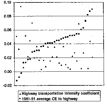
The first test we conducted was to calculate the correlation coefficient between the 35 industries' cost elasticities with respect to highway capital in Nadiri's study and the same industries' highway transportation intensities from TSA 1992. Since cost elasticity and highway transportation intensity have different signs, we would expect a large negative correlation coefficient if the initial hypothesis is true. The correlation coefficient resulting from our calculation was 0.269. This correlation coefficient was not only small, but also had a wrong sign. We were forced to accept the conclusion that there is no correlation between Nadiri's estimates of industry cost elasticities and industrys' highway transportation intensity estimates from TSA 1992. This result is evident in the scatter plot presented in Figure 1.

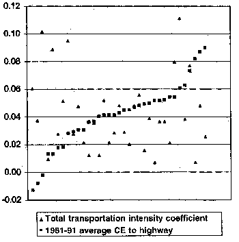
A second test we conducted was to calculate the correlation coefficient between the 35 industries' cost elasticities with respect to highway capital in Nadiri's study and the same industries' total transportation intensities from TSA 1992. We suspected that highway transportation intensity of an industry might not be a good indicator of the marginal benefit of highway capital to that industry. The reason is that highway is only one of the transportation modes, and there is high substitutability between highway transportation and other modes, such as rail transportation and air transportation. An industry with a low highway transportation intensity might benefit greatly from highway investment and increased productivity of highway transportation services, because its total transportation intensity is high. The industry may substitute another mode with highway to fully take advantage of increased productivity in highway transportation. Hence, total transportation intensity might be a better indicator of marginal benefit of highway capital to an industry.

Figure 1: Correlation Between Cost Elasticity and Highway Transportation Intensity Coefficient (0.269)

However, the result of our second test also showed no correlation between Nadiri's estimates of industry's cost elasticities and industry's total transportation intensity estimates from TSA 1992, either. The correlation coefficient between industry's cost elasticity and industry's total transportation intensity was very small (0.173) and not correctly signed. Figure 2 presents the result of the second test.

Figure 2: Correlation Between Cost Elasticity and Total Transportation Intensity Coefficient (0.173)

Modified Hypothesis

Cost elasticity with respect to highway capital is highly correlated with industry's logistic cost. Industry with high logistic cost would be expected to have large cost elasticities with respect to highway capital and industries with low logistic cost would be expected to have small cost elasticities.

The rejection of our initial hypothesis was against our intuition and led us to think deeper about the underlying mechanism through which highway capital affects industry production. The next idea we explored was that in addition to increasing the efficiency of highway transportation, and hence reducing transportation cost, highway capital benefits industry production by enabling businesses to organize their production in new and different ways. "Just-in-time" inventory practices are a good example of a mechanism through which highway capital benefits industry production in more ways than just reducing transportation cost. The "bottom line" interest of businesses to reduce total production cost and cost elasticities is in fact a measure of the change in total production cost (not just transportation cost). Therefore, more efficient transportation may actually increase rather than decrease the share of transportation cost in total production cost as business substitutes transportation for other production inputs. We asked, within an integrated production system, which subsystem will be affected most by changes in transportation? Our answer was the logistics system. Transportation is an important link of the logistic chain. Changes in transportation characteristics, such as speed, reliability, and flexibility, directly affect the way that business organizes components of the distribution system, which in turn affects total logistics costs. Therefore, the share of logistic cost in an industry's production cost might be better than the share of highway transportation cost as an indicator of the magnitude of potential benefits that the industry might receive from increases in highway capital.

To test the modified hypothesis, we constructed two logistic cost proxies using data from TSA 1992. In Proxy A, the total transportation intensity measure is augmented by the TSA cost coefficients for the finance, insurance, and real estates sector, the other services sector, and the government enterprise sector. In Proxy A, the highway transportation intensity measure is augmented by the TSA cost coefficients for the finance, insurance, and real estates sector, the other services sector, and the government enterprise sector. The reason for these augmentations is that cost coefficients for these three sectors capture the most logistics costs. The cost coefficient for the finance, insurance, and real estates sector includes the costs of motor vehicle insurance, commodity broker and insurance, real estate broker, and warehouse rents. The cost coefficient for the other services sector includes the costs of automotive rental and leasing, automotive repair shops and services, and automotive parking and car washing. The cost coefficient for the government enterprises sector, includes the costs of postal services and government passenger transit.

Results of Testing the Modified Hypothesis

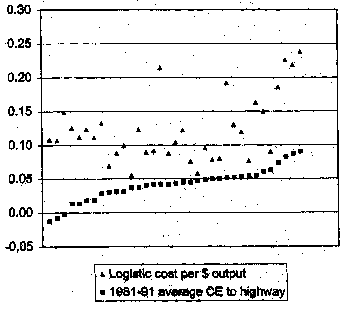
We again started our test by calculating the correlation coefficients. The correlation coefficient between the 35 industries' cost elasticity with respect to highway and logistic cost Proxy A was -0.46, while the correlation coefficient for Proxy B was -0.45. Not only did the absolute value of the correlation coefficients increased significantly, but, more importantly, the coefficients also were correctly signed. Since Professor Nadiri's cost elasticity estimates for metal mining (2), nonmetallic mining (5), and leather and leather products are admittedly questionable, they are considered as outliers. When these three industries were removed from the data set, the correlation coefficient for Proxy A increased to -0.55 and correlation coefficient for Proxy B increased to -0.57. The corresponding R² for the two coefficients are 0.31 and 0.32, respectively, indicating that about one-third of the variance in cost elasticity across industries reflects or can be explained by the variance in industries' logistic costs. These results are shown in Figure 3 and Figure 4.

The second step was to test whether the correlation coefficients would be statistically significant. We ran a simple regression analysis between cost elasticity and logistic cost proxies, which automatically generated F-test results about the correlation coefficients. The F value for the correlation coefficient of Proxy A was 13.2. And the F value for the correlation coefficient of Proxy B was 14.3. Both are about two times as large as the critical value (7.56) of F test with degrees of freedom of (1, 30) and significance level of 0.01. In other words, the F-test states that the modified hypothesis can be accepted with 99 percent confidence.

Figure 3: Correlation Between Cost Elasticity and Logistic Cost Coefficient (Proxy A, -0.458)

Conclusion

1. Highway capital affects industry production in much broader ways than just reducing highway transportation cost. Faster, more flexible, and more reliable highway transportation enables industries to organize productions in new and different ways.
2. There is no correlation between Nadiri's estimates of industry cost elasticities with respect to highway capital and the transportation intensity coefficients (total or highway only) from TSA 1992. However, there is statistically significant correlation between cost elasticity with respect to highway capital and total logistic cost. These findings indicate that the share of logistics cost in an industry's production cost might be a better object of analysis than the share of highway transportation cost in future researches about the magnitude of potential benefits from increases in highway capital investment.

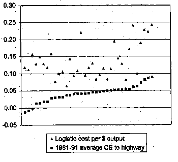
Figure 4: Correlation Between Cost Elasticity and Logistic Cost Coefficient (Proxy B, -0.447)

Table 2: Correlation Analysis of Cost Elasticity of Nadiri Study with Industry Transportation Intensity Coefficients of TSA 1992

Correlation	Cost Elasticity of Nadiri study	Cost Elasticity of Nadiri study**
All transportation intensity coefficient	0.17	0.01
Highway transportation intensity coefficient	0.27	0.02
Total intermediate input coefficient	0.20	0.21
Logistic cost coefficient (Proxy A)	-0.46	-0.55
Logistic cost coefficient (Proxy B)	-0.45	-0.57
Industry use of all transportation services	-0.66	-0.72
Industry use of highway transportation services	-0.62	-0.70

^** Correlation coefficients were based on a modified data set in which three industries with positive signs for cost elasticity were removed. These three industries were metal mining, nonmetallic mining, and leather and leather products.

Table 3: Results of Statistical Significance Test

A. Regression of cost elasticity with logistic cost coefficient (proxy A)

Correlation
Multiple R	0.553
R Square	0.306
Adjusted R Square	0.282
Standard Error	0.016
Observations	32

ANOVA

	df	SS	MS	F	Significance F
Regression	1	0.00353	0.00353	13.20131	0.00103
Residual	30	0.00802	0.00027
Total	31	0.01155

	Coefficients	Standard Error	t Stat	P-value	Lower 95%	Upper 95%
Intercept	-0.0176	0.0083	-2.12139	0.04226	-0.03455	-0.00066
X Variable 1	-0.20698	0.05697	-3.63336	0.00103	-0.32331	-0.09064

B. Regression of cost elasticity with logistic cost coefficient (proxy B)

Correlation
Multiple R	0.569
R Square	0.324
Adjusted R Square	0.301
Standard Error	0.016
Observations	32

ANOVA

	df	SS	MS	F	Significance F
Regression	1	0.00374	0.00374	14.34765	0.00068
Residual	30	0.00781	0.00026
Total	31	0.01155

	Coefficients	Standard Error	t Stat	P-value	Lower 95%	Upper 95%
Intercept	-0.01939	0.00755	-2.56836	0.01544	-0.03480	-0.00397
X Variable 1	-0.21611	0.05705	-3.78783	0.00068	-0.03262	-0.09959