Traffic Monitoring Guide

Appendix G. NORTH CAROLINA DEPARTMENT OF TRANSPORTATION CLUSTERING METHODOLOGY FOR NC TRAFFIC DATA INPUTS FOR MEPDG

G.1 INTRODUCTION

The recommended process for implementation of the Mechanistic-Empirical Pavement Design Guide (MEPDG) involves the development of data inputs that reflect the conditions experienced at the design locations. This requires some element of both site specific and regional inputs to support an effective design process. Data inputs include climate, soil, materials, and traffic categories. Agencies in the development of these inputs must decide what level of detail will be needed to produce a reliable pavement. North Carolina traffic inputs were developed based on a research study conducted by North Carolina State University for the North Carolina Department of Transportation. The study included the evaluation of data from 44 Weigh In Motion (WIM) stations located across North Carolina. The process used to develop the traffic data inputs from this resource involved:

• Quality control of vehicle class and truck weight data;
• Sensitivity analysis of design models to traffic inputs;
• Clustering analysis of the WIM based traffic inputs; and
• Selection criteria for using clustered based traffic data.

A brief explanation of the factors considered in developing traffic inputs, sensitivity of design models to North Carolina inputs, the clustering methodology used, and the results they produced is provided. A description of the method developed to select grouped data for input into the design process is provided also. Key decisions made during the process required to develop these traffic inputs are discussed.

This paper is a brief synopsis of information provided in the final report of the research study related to generating clustered data sets. It is not intended to convey the complete findings of that study. All of the tables and figures are taken directly from the final report

The results of the analyses and factors developed may be fairly unique to North Carolina. The process used to develop the analysis, the methods used to cluster the data, and the considerations given and solutions selected to address the issues encountered during the research can be transferred to similar studies. The development of clustered data sets for the MEPDG can be complex and agencies involved in this type of development will have to make many choices. The experience in North Carolina may provide some insight into how best to make those choices.

G.2FACTORS AFFECTING CLUSTERING REQUIREMENTS

A number of factors are critical to development of the analysis of the traffic data collected at WIM stations effectively. Factors that affected the development process were:

• Design Level – The NCDOT has selected Level 2 traffic inputs as the basis for most pavement designs. This is due to the impracticality of collecting site specific traffic for all inputs (Level 1) because of time and cost constraints. Level 1 traffic inputs will be used when a WIM site falls on or near a project. Level 3 inputs may be used on a limited basis and are supported also.
• WIM Data Types – The type of data collected at WIM stations by the NCDOT is continuous vehicle classification counts and truck weight measurements. These data resources provide the basis for Hourly Distribution Factors (HDF), Monthly Adjustment Factors (MAF), Vehicle Class Distributions (VCD), and Axle Load Distribution Factors (ALF). These statistics were generated for each station (Level 1) and clustering was performed to generate grouped factors for Level 2 inputs. Other statistics generated from this data but not clustered were average axle types by vehicle class and average axle spacing by axle type. The other traffic inputs to the MEPDG are either site specific (AADTT and growth) or national defaults are used (tire pressure, lane wander, etc.).
• Model Sensitivity – A sensitivity analysis identified which models are sensitive to each of the WIM based traffic inputs. When any of the models were found to be sensitive to a process, a clustering analysis was performed to generate grouped inputs. When all models were found not to be sensitive to an input, a statewide average was generated as the default values for that input.

These factors directly impacted the requirements for clustering a data type and influenced the process. Other factors affecting the clustering analysis of individual data inputs are provided below.

G.3SENSITIVITY OF MODELS TO NORTH CAROLINA TRAFFIC DATA

The MEPDG process requires significantly higher levels of data inputs than legacy pavement design processes. A key component to understanding how best to use the process is an understanding of how traffic inputs, and in particular, North Carolina inputs, impact the output of the design models. This provides the basis for simplifying the process, where practical, and ensures the appropriate level of detail is input to generate reliable pavement designs.

The sensitivity analysis was performed using representative LTPP sites located in North Carolina as the structural and material data is available for input. The range of values for HDF, MAF, VCD, and ALF found in the data at the 44 WIM sites was used. Only one input was changed at a time and all models in the design process were run when evaluating sensitivity. When a model output changed enough to exceed a threshold specified by the pavement designers, that model was identified as sensitive to the input being evaluated. The results of the sensitivity analysis are provided in Table G-1.

The researchers found that the longitudinal cracking model for flexible pavements did not produce outputs consistent with what is observed in the performance of North Carolina pavements. Although this model was found to be sensitive to some traffic inputs, the unreliability of the outputs resulted in the exclusion of this model’s sensitivity from consideration in the clustering process.

TABLE G-1 SENSITIVITY OF MEPDG TO NORTH CAROLINA BASED TRAFFIC INPUTS

	Flexible Pavement				Rigid Pavement (JPCP)
	Total Rut Depth (in)	Fatigue Cracking (%)	Longitudinal Crackinga (ft/mile)	IRI (in/mile)	Faulting (in)	Slabs Cracked (%)	IRI (in/mile)
HDF	no	no	no	no	no	no	no
MAF	no	no	yes	no	no	no	no
VCD	yes	yes	yes	yes	no	no	yes
ALF	yes	yes	yes	yes	yes	no	no

Source: North Carolina Department of Transportation

There are naturally occurring clusters in the HDF and MAF data sets. The lack of sensitivity of the models to these inputs (excluding the longitudinal cracking results), based on North Carolina data, eliminates the need for clustering data for these inputs. Statewide average values were generated using the average of the 44 WIM data sets for these inputs to simplify the design process.

The VCD data is a key input into the design process as models for both flexible and rigid pavements show sensitivity to this input. The flexible pavement models are sensitive to the ALF input but rigid pavements models are not sensitive. Based on these results, clustering analysis was performed on the VCD and ALF data to generate grouped data sets for Level 2 inputs.

G.4 HOURLY DISTRIBUTION FACTOR INPUT

The MEPDG models were found to not be sensitive to the range of HDF calculated for the 44 WIM stations in North Carolina. This allows the use of a single set of HDF for input into the pavement design process based on the average of the individual HDF. Figure G-1 provides a plot of the average HDF that is used in the design process.

FIGURE G-1 NORTH CAROLINA HOURLY DISTRIBUTION FACTORS

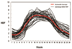
Source: North Carolina Department of Transportation.

G.5 MONTHLY ADJUSTMENT FACTOR INPUT

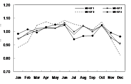
Similarly, the MEPDG models were not sensitive to the range of MAF experienced at North Carolina’s 44 WIM stations. WIM Stations 533 and 560 were identified as outliers based on a principal component analysis and were excluded from further analysis. A statewide average based on the remaining 42 individual MAF was generated to provide a single set of MAF as input into the pavement design process. Figure G-2 provides a plot of the average MAF that is used in the design process with the outliers that were excluded identified.

FIGURE G-2 NORTH CAROLINA MONTHLY ADJUSTMENT FACTORS

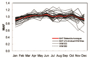
Source: North Carolina Department of Transportation.

G.6 VEHICLE CLASS DISTRIBUTION INPUT

Due to the sensitivity of most of the models to VCD inputs, a clustering analysis was performed on this data. The VCD is the distribution of the AADTT into the 10 FHWA truck classes. Therefore, the method used should support evaluating the patterns observed between the ten classes of trucks in this input. The clustering methodology used was:

• Statistic – VCD Distribution of the 10 FHWA Truck Classes;
• Technique – Agglomerative Hierarchal Clustering; and
• Measure – Sum of Least Squares of the Differences in VCD Values.

This technique starts with each WIM site as an individual cluster and calculates the difference in VCD between each pair of clusters. The difference is calculated between each of the 10 VCD percentages, each of these values is squared, and the total is summed. The clusters having the lowest value of this measure are the most similar and are grouped together. The VCD for the new cluster is the average of the component VCD making up that cluster. This process is repeated until all 44 WIM sites are clustered into a single group. The stopping level was determined by applying a metric proposed by Mojena. As iterations of the clustering process are performed, there is a loss in the uniqueness of the patterns. The new clusters created are more generalized and greater amounts of variability are introduced into the clusters. The Mojena metric identifies the most suitable number of clusters based on the level of variability in the data set. Three clusters were identified for the VCD input and are shown in Figure G-3.

FIGURE G-3 NORTH CAROLINA VCD CLUSTERS

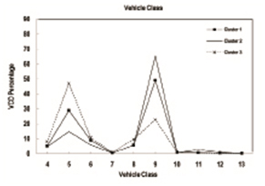
Source: North Carolina Department of Transportation.

As VCD is a distribution of total trucks at a location, it corresponds that as one class of vehicle increases, the other classes decrease. In the patterns represented by the clusters, Cluster 2 has a significantly higher proportion of Multi Unit (MU) trucks, found in Class 8 to 13, than Single Unit (SU) trucks, found in Class 4 to 7. Conversely, Cluster 3 has significantly higher proportion of SU trucks than MU trucks. Cluster 1 falls between the two other clusters with slightly higher MU trucks than SU trucks. The type of routes associated with these clusters is consistent with the patterns. Cluster 2 includes interstate and higher order U.S. routes that serve long distance trips, provide a higher level of mobility, and serve major markets. There are a higher proportion of MU trucks in this cluster due to the longer trip lengths this type of vehicle travels, the large markets served, and the regional connections they provide. Cluster 2 includes mostly State and local routes with lower mobility and limited connectivity that serve primarily the shorter business day trips associated with the SU trucks. Cluster 1 is a mix of route types including interstate routes in urban areas where there is a higher level of business day travel by SU trucks than rural interstate locations. It includes U.S. and other routes where mobility is higher than local routes but they have a lower level of long haul trips because of the smaller markets served and lower levels of connectivity they provide.

G.7 VEHICLE CLASS SEASONAL FACTOR GROUPS

A basic input into the MEPDG process is Annual Average Daily Truck Traffic (AADTT) for a project. The NCDOT collects vehicle classification counts for each project as the basis for identifying base year conditions. The counts collected classify traffic into the FHWA 13 Class scheme. This provides not only a measure of total trucks for AADTT, but the distribution of trucks between the 10 truck classes required for the VCD estimate. Based on the higher sensitivity of the models to the VCD input, and the availability of data for each project, it was decided to estimate project specific VCD based on the short term class counts instead of using the generalized values from the VCD cluster analysis

A key element in using short term class counts for generating AADTT and VCD estimates is seasonally factoring the count data to annualized values. A clustering analysis for the purpose of factoring short term class counts was performed. The observed pattern in the daily distributions of truck volumes through the year was performed for the 44 WIM stations available. The NCDOT processes and reports class data by aggregated vehicle class groups. Single Unit trucks (Class 4 to 7) have similar business day travel patterns and Multi Unit trucks (Class 8 to 13) have similar long haul travel patterns. This method of developing and applying seasonal factors using aggregated vehicle classes is supported by research and is a recommended practice in the Traffic Monitoring Guide. Key steps taken prior to clustering the data were:

1. Data Screening – The class volume data collected at the WIM stations was evaluated for daily truck distributions by day of week by month. The daily truck distributions (VCD) for each day of week within the same month were compared to identify the recurring or typical pattern for that day. Any day that exhibited a pattern different from the recurring pattern was flagged as an atypical pattern. This produced 7 day of week patterns for each month for a total of 84 sets per WIM station.

2. WIM Station Factors – The NCDOT collects short term counts on typical travel days. The factors used in this process reflect this practice. AADTT and Monthly ADTT (MADTT) were calculated for SU and MU truck class groups for each station using the method recommended in the Traffic Monitoring Guide. This includes using both typical and atypical days in these averages. Average day of week daily truck volumes for typical days were calculated for SU and MU trucks. Seasonal factors were calculated using the ratio of the AADTT to the average typical day of week volumes for SU and MU factors for each day of week for each month. The statistics generated for each station were:

• AADTT (1), Annual VCD (1), Monthly VCD (12);
• AADTT SU (1), MADTT SU (12), Day of Week Factor SU (84); and
• AADTT MU (1), MADTT MU (12), Day of Week Factor MU (84).

This data is suitable for factoring short term counts collected on typical days when at or near a WIM station location and was used as the basis for the clustering process for generalized class seasonal factors.

The clustering methodology used for seasonal factor development accounts for the truck volume seasonality experienced in North Carolina. A two stage procedure is used in development of seasonal factors:

Phase 1 – Analysis of Monthly VCD Seasonal Patterns

• Step 1: Evaluate Principal Components for Outliers;
• Step 2: Perform Monthly Clustering Analysis; and
• Step 3: Identify Common Groupings.

Phase 2 – Analysis of SU/MU Seasonal Patterns

• Step 1: Evaluate MADTT/AADTT Plots by SU/MU;
• Step 2: Evaluate Principal Components for Outliers; and
• Step 3: Audit Confidence Intervals of Seasonal Factors.

Since a primary output of the factoring process is VCD, this attribute, and how it varies through the year, is used as the first stage in the development of seasonal factor clusters. The second stage involves the analysis of each aggregated truck class (SU/MU) for their underlying patterns within the VCD patterns. This generates groupings specific to what is being factored.

Phase 1 – Analysis of Monthly VCD Seasonal Patterns

Step 1: A principal component analysis was performed to identify which components of the VCD are most important, or account for most of the variability in the data. In the case of VCD, the components are the 10 truck classes comprising the distribution. This portion of the analysis determined that Class 4, 5, 6, 8, 9, and 11 were the classes that account for most of the variability in the data during the year. Individual classes determined to be principal components for a particular month will vary by month. The results of this analysis are provided in Table G-2.

TABLE G-2 PRINCIPAL COMPONENTS OF NORTH CAROLINA MONTHLY VCD

Month	Vehicle Class
	4	5	6	7	8	9	10	11	12	13
January
February
March
April
May
June
July
August
September
October
November
December

Source: North Carolina Department of Transportation.

The PCA results were used to identify outliers to the principal components and 2 WIM stations were excluded due to their significantly different characteristics. The remaining 42 WIM stations were used in the clustering analysis.

Step 2: A monthly clustering analysis process was employed using the results of the PCA. This involved use of the following methodology:

• Statistic – Principal Monthly VCD Components by month;
• Technique – Agglomerative Hierarchal Clustering; and
• Measure – Sum of Least Squares of the Differences in Monthly VCD Values.

A cluster analysis was performed for each month to identify groupings for that month. In each case, 3 groupings were identified for each month.

Step 3: The groupings were compared from month to month to determine if the same sites were being clustered across the year. Three groupings were identified where the same sites were grouped together in at least 11 of the 12 months. These groupings represent WIM stations with the same pattern in changes in VCD across the year

Phase 2 – Analysis of SU/MU Seasonal Patterns

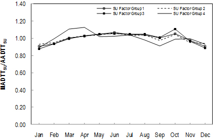
Step 1: The seasonal pattern of each of the aggregated truck classes should be evaluated for consistency within the groupings identified in Phase 1. The ratio of MADTT to AADTT is calculated for SU and MU truck groups as the basis for identifying their seasonal pattern. Plots of this statistic for all WIM stations within a factor group were generated for SU and a separate set of plots for MU to make this comparison. WIM stations found to have an inconsistent plot as compared to the common pattern were excluded from the group. This resulted in the exclusion of some WIM sites and the extraction of a fourth grouping of sites located on the I-95 corridor. The unique seasonal pattern on the I-95 corridor resulted in a separate fourth seasonal factor group for both SU and MU classes.

Step 2: A separate principal component analysis of the ratio of MADTT to AADTT for SU and MU was performed. This process identified individual WIM stations that are not consistent with the pattern in principal components among a group. These were eliminated from the grouping when they occurred.

Step 3: Seasonal factors for each group are evaluated for the confidence interval obtained in them. These are calculated for each month of seasonal factors. Any WIM station whose seasonal factors exceed the 95% confidence level in multiple months were eliminated from the grouping. This occurred once in one of the SU factor groups.

The results of this two phase process are a set of seasonal factor groups for SU and MU class groups. The results are represented in the plot of the average monthly MADTT/AADTT ratio for each factor group in Figures G-4 and G-5.

In general, selection of a factor group/station for application of seasonal factors to a portable vehicle classification (PVC) count has been correlated to the route the count is located on and the class distribution identified in the count. The route location is used to determine if the I-95 group factors are to be used or the count is located on the same corridor as a WIM station and the seasonal factors from that individual WIM station should be used. If the route location is found not to be the determining characteristic, then the class distribution found in the count is used as the basis for selecting a seasonal factor group. The correlation between the distribution of total trucks between SU and MU types counted during a 48 hour short term count period and the seasonal factor group assignment is determined using the criteria provided in Table G-3.

FIGURE G-4 MADTT/AADTT FOR NORTH CAROLINA SINGLE UNIT TRUCK SF GROUPS

Source: North Carolina Department of Transportation.

FIGURE G-5 MADTT/AADTT FOR NORTH CAROLINA MULTI UNIT TRUCK SF GROUPS

Source:North Carolina Department of Transportation.

TABLE G-3 ASSIGNMENT CRITERIA OF PVC TO NORTH CAROLINA SEASONAL FACTOR GROUPS

SU Trucks/Total Trucks		SU Group
Min (=)	Max (<)
0.09	0.34
0.34	0.50
0.50	0.71
MU Trucks/Total Trucks		MU Group
Min (=)	Max (<)
0.67	0.92	1
0.50	0.67	2
0.29	0.50	3

Source: North Carolina Department of Transportation.

The criteria provided in Table G-3 does not cover the extreme ends of the spectrum of distributions; the WIM monitoring practice in North Carolina has been to monitor those routes that have a moderate to significant volumes of trucks. The extreme end of the range represents primarily low volume locations or facilities serving specialized land uses. It is assumed that these types of facilities will exhibit similar seasonal patterns as the adjacent seasonal group. This assumption is applied by the following rules:

If SU/Total < 0.09 assign SU Group 1

If SU/Total ≥ 0.71 assign SU Group 3

If MU/Total < 0.29 assign MU Group 3

If MU/Total ≥ 0.92 assign MU Group 1

The NCDOT plans to install monitoring stations at the extreme ends of these distributions to develop a more complete understanding of truck travel and a comprehensive method for seasonal factoring of truck data.

G.8 AXLE LOAD DISTRIBUTION FACTOR INPUT

The sensitivity analysis showed that the flexible pavement models were sensitive to the Axle Load Distribution Factor (ALF) input. An analysis of the per vehicle truck weight data collected at WIM stations was required to develop Level 2 inputs. This involved performing of the following tasks:

1. Convert axle spacing and axle weight measurements into axle load data;

2. Generate ALF for each WIM station (Level 1 inputs);

3. Identify the ALF factors that most impact the pavement design process;

4. Perform a principal component analysis to eliminate outliers/aggregate load bins;

5. Perform a clustering analysis to identify groups of similar ALF patterns; and

6. Evaluate the characteristics of the groups to define a method for selecting ALF.

The ALF data is an input that influences the flexible pavement design process. The research team had two issues to consider that impacted the development process:

• Quality Control of Axle Spacing/Weight Measurements – The QC method used was a rule based evaluation of individual measurements or a combination of measurements to eliminate illogical values. There are additional QC methods available that can be used to identify misclassified trucks based on axle weights. The NCDOT classifies vehicles based on the number of axles and their spacing. This is not an axle weight based algorithm. This algorithm is used in all devices that collect vehicle classification data, including portable classifiers and WIM stations. The basis for AADTT and VCD inputs for pavement design are counts collected with portable classifiers. The basis for the classifications in the ALF should be identical to those used for other classification based inputs. Although these are errors in the ALF classifications, they are measurements of valid loadings on the pavement. As long as the classification algorithms are identical for all inputs, the appropriate loadings will be generated by the models, even if applied through a different class of truck. Therefore, quality control of the axle weight data did not include validation of vehicle classification based on axle weights or validation of axle weights based on vehicle classification.
• Damage Based Clustering – The research team advised that the ALF clusters would be more reliable if based on the relative level of pavement damage caused by each ALF input. This required identifying not only which axle types caused the most damage, but the weight ranges (load bins) for those axle types that accounted for the majority of the loads being applied. Once these critical inputs were identified, the clustering process was based on them to avoid influencing the results on non-essential or nominal ALF factors. The technique was developed in Step 3 of the ALF development process.

These decisions had a significant impact on the ALF development process. Without considering these issues and addressing them appropriately, the ALF factors generated would be less reliable and could require more expensive pavement designs to adjust for this limitation

Step 1 – Convert WIM Data into Axle Load Data

This process required the identification of axle types from the axle spacing data and combining of axle weights when an axle type included two or more axles. Although the original MEPDG software includes a module to generate this data, the class algorithm used by the NCDOT is moderately different than the default values used in the module. The truck spacing/weight data was processed using the ASTM E 1572-93 methodology for identification of axle types from axle spacing data. However, the spacing thresholds were adjusted to reflect North Carolina’s classification algorithm. The spacing ranges applied are provided in Table G-4.

TABLE G-4 NORTH CAROLINA AXLE SPACINGS DEFINING AXLE TYPES FOR ASTM E 1572-93

	Axle Spacing (inches)
Axle Count	24-39	40-96	97-150	118-192	193+
1	Single	Single	Single	Single	Single
2	Single-2	Tandem-2	2 Singles	2 Singles	2 Singles
3		Tandem-3	Tridem	Tridem	2 or 3 confg.
4		Tandem-4	Tridem-4a	Quad-4	Quad to 288
5		Tandem-5	Tridem-5a	Quad-5	Quad to 384
6			Tridem-6a	Quad-6	Quad to 480

Source:  North Carolina Department of Transportation.

Once an axle type is defined, the weight for that axle type is generated. Axle types with a single axle are assigned the weight of that axle. Axle types with 2 or more axles are assigned the sum of the individual axle weights. The process converts each weight record to an axle load record including vehicle classification and the individual axle types and their associated weights for all axle types identified for that truck. This process was applied to each WIM station separately to allow generation of station specific ALF.

Step 2 – Generate ALF for each WIM Station

The converted axle load data was used as input into this process. Each record in the axle load data was disaggregated by each individual axle type and then categorized by the weight range it falls in. The ALF are based on frequency distributions of axle types for each vehicle class stratified by weight ranges. The factors are the ratio of the number of an axle type occurring within an individual weight range to the total number of that axle type occurring in all weight ranges. Not all axle types occur in all truck classes (e.g. Class 5 has single axles only). This is dependent on the variety of axle configurations that occur within a vehicle class. A set of ALF was generated for each of the 44 WIM stations available.

Step 3 – Identify Critical ALF

The use of a multidimensional clustering technique was selected as it supports evaluation of multiple sets of data elements. The advantage of this technique is that the multiple sets of ALF used in generating loadings on a pavement are incorporated in the cluster analysis. The limitation of this technique is the complexity of working with so many data sets and the potential for influencing the results based on data that has high variability but contributes little to the design process. To reduce the potential for this, a method was developed to identify those ALF inputs critical to the design process.

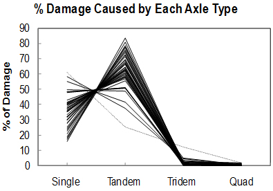
The method used involved quantifying the distribution of damage occurring during the design life of a pavement between the axle types used in the ALF. The researchers developed the Damage Factor metric that is the ratio of the fatigue damage caused by a particular axle type within a particular weight range (called a load bin) to the fatigue damage caused by an 18-kip Equivalent Single Axle Load. The Fatigue Cracking model was used to develop these factors as 90% of pavements in North Carolina are flexible pavements and this is the primary mode of failure experienced in North Carolina for this pavement type. The damage factors were developed for each WIM station and are unique to the conditions experienced at each station. The output generated from factoring the axle types/loads to ESALs provides the basis for making comparisons and developing an understanding of the critical ALF. The result of this process is provided in Figure G-6 which shows the contribution each axle type makes to total damage at each of the 44 WIM stations.

FIGURE G-6 PERCENT DAMAGE BY AXLE TYPE AT NORTH CAROLINA WIM STATIONS

Source: North Carolina Department of Transportation.

It was determined that 98% of total damage is caused by Single and Tandem axle types. This characteristic allowed the exclusion of Tridem and Quad axle types from the clustering analysis. Additionally, the individual load bins for the Single and Tandem axle types were evaluated for two characteristics:

• Did the load bin include more than 1% of all loadings for that axle type?
• Did the load bin contribute more than 1% of all damage for that axle type?

If either of these conditions were met, the load bin was considered significant and retained for the cluster analysis. If neither of these conditions were met, the load bin was excluded. Table G-5 specifies the load bins retained based on this evaluation.

TABLE G-5 LOAD BINS RETAINED FOR ALF CLUSTER ANALYSIS

Single	Tandem	Tridem	Quad
3 KIPS-21 KIPS	6 KIPS-50 KIPS	None	None

Source: North Carolina Department of Transportation.

Step 4 – Analyze Principal Component

The analysis involved the evaluation of the ALF to determine principal components. This information was used as the basis for identifying WIM stations with ALF that were significantly different and were excluded as outliers. Two stations were identified as outliers and the remaining 42 WIM stations were used in the clustering analysis.

A second principal component analysis was performed to identify aggregations of load bins, within each axle type, that could be used in the clustering process to minimize the affect of variability in individual load bins. The results of this analysis are presented in Table G-6.

TABLE G-6 RESULTS OF THE PRINCIPAL COMPONENT ANALYSIS FOR SINGLE-TANDEM ALF

Principal Component	Aggregated Load Bin	Variance	Cumulative Variance
1	Heavy Tandem (22-50 KIPS)	74.82	0.65
2	Light Tandem (6-20 KIPS)	24.10	0.86
3	Single(11-20 KIPS)	8.83	0.94
4	Single (6-10 KIPS)	5.59	0.99
5	Single (3 KIPS)	1.42	1.00
6	Single (4 KIPS)	0.15	1.00
7	Single (5 KIPS)	0.03	1.00

Source: North Carolina Department of Transportation.

Step 5 – Evaluate Cluster Analysis of ALF

A two dimensional clustering technique was used to evaluate the 44 WIM station ALF to identify stations with similar loading patterns. The analysis was based on the Single and Tandem axle types for the 7 aggregated load bins found to be significant.

• Statistic – ALF for Single and Tandem Axle Types for 7 Aggregated Load Bins;
• Technique – Two Dimensional Hierarchal Clustering; and
• Measure – Sum of Least Squares of the Difference in ALF by axle type/load bin.

This technique requires the calculation of the difference between the ALF for each of the 7 aggregated load bins for a WIM site and the average value of all WIM sites for each load bin. This is done for all WIM stations in a cluster being considered. Each of those differences is squared and then summed to provide a single variability metric for the proposed cluster. This is done for all potential clusters in the step being evaluated and the cluster with the lowest value; representing the least amount of variability is the cluster identified for grouping for that step. This process is repeated until all WIM sites are grouped into a single cluster. Similar to the previous clustering analyses, the metric introduced by Mojena is the method used in identifying the appropriate number of clusters for the analysis.

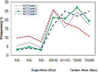
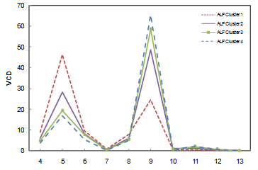
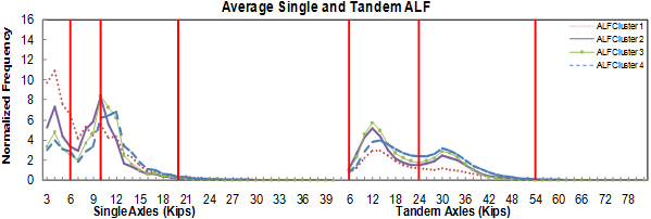
The clustering analysis identified 4 clusters of WIM stations with similar ALF patterns. Figure G-7 provides the average Single and Tandem ALF (plotted as single line) using the aggregated load bins for each of the 4 clusters for comparison. The average VCD for each of the clusters is provided in Figure G-8. This plot helps us to understand the patterns observed in Figure G-7. Observations based on these two figures include:

• The VCD for Cluster 1 exhibits a much higher proportion of SU trucks compared to MU trucks; this correlates with the higher frequency of the single axle load bins and a lower frequency in the tandem, especially the heavy tandem bin as compared to the other three clusters;
• The VCD for Clusters 2, 3, and 4 all have higher proportion of MU trucks than SU trucks; these proportions increase as you progress from Cluster 2 to 4; this correlates to the higher frequency in the tandem load bins; and
• The VCD for Cluster 4 has the highest proportion of MU trucks; this correlates with the highest proportion of heavier single and heavy tandem load bins.

FIGURE G-7 AVERAGE AGGREGATED SINGLE-TANDEM ALF FOR TWO-DIMENSIONAL CLUSTERS

FIGURE G-8 AVERAGE VEHICLE CLASS DISTRIBUTION FOR TWO-DIMENSIONAL ALF CLUSTERS

Source: North Carolina Department of Transportation.

It appears that as the proportion of MU trucks increases, the frequency in the heavier load bins increases also. This indicates that the type of facilities that serve long haul MU trucks well will experience the heaviest loading. Although this conclusion can be somewhat intuitive, it is validated by the results of the cluster analysis.

A plot of the average ALF for Single and Tandem axle types are provided in Figure G-9. These are the values used for input into the pavement design process. The average ALF for Tridem and Quad axle types were generated using the same WIM sites in each cluster to provide these inputs also.

FIGURE G-9 AVERAGE SINGLE AND TANDEM ALF FOR NORTH CAROLINA

Source: North Carolina Department of Transportation

Step 6 – Develop Method for ALF Group Selection

The results of the analysis explained in the previous steps provide the axle loading inputs needed for the pavement design process. To use these resources effectively, the designer will need to select the ALF most suitable to the traffic anticipated to travel over the pavement being designed. The research team performed an evaluation of the characteristics of the WIM stations that comprise each cluster to identify attributes that may explain why they have similar loading patterns. The same attributes for the pavement design location could then be used as the basis for selecting the appropriate ALF. Some of the attributes evaluated included:

Quantitative – AADT, AADTT, VCD, SU%, MU%, Class 5%, Class 9%

Qualitative – Route Type, Route Category, Facility Type, Functional Classification, Geographic Region, Area Type

There are some definitive quantitative measures that will determine specific ALF selections. These are based on the Class 5 and 9 percentages of total trucks calculated from the short term counts collected for a project. However, these statistics have overlap between two to three ALF groups in some ranges. In these cases, the designer will need to use a qualitative attribute, the route category, to select between the overlapping ALF. The route category types are Primary Arterial, Secondary Arterial, Collector, and Local routes. This is very similar to the Functional Classification attribute but is selected in the context of how a route will serve truck trips instead of total traffic. The designer must exercise some judgment when selecting the appropriate route category for a project. The ALF selection process is provided in Table G-7.

TABLE G-7 SELECTION CRITERIA FOR NORTH CAROLINA ALF

Parameter	Route Category	ALF
Project Route Location = WIM Route Location	N/A	WIM ALF
30 ≤ Class 5% < 54 and 4 ≤ Class 9% < 44	N/A	ALF Group 1
3 ≤ Class 5% < 18 and 68 ≤ Class 9% < 85	N/A	ALF Group 4
24 ≤ Class 5% < 37 and 44 ≤ Class 9% < 68	Primary Arterial	ALF Group 4
	Collector	ALF Group 2
10 <= Class 5% < 24 and 44 <= Class 9% < 68	Primary Arterial	ALF Group 4
	Secondary Arterial	ALF Group 3
	Collector	ALF Group 2

Source: North Carolina Department of Transportation.

If the data for Route Location, Class 5%, Class 9%, and Route Category for a project are not covered by the parameters specified in Table G-7, the designer should select the nearest match as the basis for selecting ALF. This could indicate a potential gap in the ALF data and the need to install a WIM monitoring station to provide the missing data.

G.9SUMMARY

The study analyzed WIM data sets to generate appropriate traffic inputs for the MEPDG process. The methods used to generate North Carolina data are transferable to similar analyses. The elements considered critical to development of reliable traffic inputs for MEPDG include:

• Class Algorithms – Data collected using different technologies for traffic inputs should use the same class algorithm. This eliminates inconsistencies in the data that may result in a less reliable design process.
• Quality Control of Data – All data collection processes will capture anomalous data sets. Agencies should have a well designed quality control process to trap anomalous data and identify when data should be excluded.
• Principal Component Analysis – It is critical to perform these type of analyses to determine what elements in a data set are critical and when individual data are not consistent with the data being analyzed and should be excluded. This step is critical to understanding how the data should be clustered.
• Clustering Methodology – The method selected should account for the statistics being generated and the component elements found to be critical. This process should be simplified when practical without adversely affecting the results. This should make it easier to develop an understanding of the types of patterns captured in the groups and why those patterns occur.
• Selection Criteria – The results of the clustering analysis can’t be used without developing a method for selecting the appropriate clustered data set to be used as an input. Objective measures are preferred as this simplifies the selection process. Multiple criteria may be required to definitively select the appropriate input.

There are many decisions made during the analysis process. These should be made based on the intended use of the data and the characteristics of the data being evaluated. If the analyst exercises care, and solicits input from traffic and pavement design experts, a reliable set of traffic inputs for the MEPDG can be developed.

G.10 REFERENCES

American Society for Testing and Materials. Standard Practice for Classifying Highway Vehicles from Known Axle Count and Spacing, ASTM E1572-93, 1994.

Stone J.R., Kim Y.R., List G. F., Rasdorf W., Jadoun F., Sayyady F., Ramachandran A., Development of Traffic Data Input Resources for the Mechanistic Empirical Pavement Design Process, NCDOT Report 2008-11, 2011.

Traffic Monitoring Guide, FHWA, U.S. Department of Transportation, May 2001.

Contact Information

Kent L. Taylor
State Traffic Survey Engineer
Traffic Survey Group
Transportation Planning Branch – NCDOT

Office Telephone: (919) 771-2520
Cell Telephone: (919) 218-4049
Fax: (919) 773-2935

E-mail: kltaylor@ncdot.gov

Mailing Address:

Traffic Survey Group
1547 Mail Service Center
Raleigh, NC 27699-1547

Delivery Address:

750 N. Greenfield Parkway
Garner, NC 27529

Link to Final Report for NCDOT 2008-11
http://www.ncdot.org/doh/preconstruct/tpb/research/download/2008-11FinalReport.pdf