U.S. Department of Transportation
Federal Highway Administration
1200 New Jersey Avenue, SE
Washington, DC 20590
202-366-4000
Traffic monitoring is performed to collect data that describes the use and performance of the roadway system. This chapter describes the types of data that should be collected, the technologies that are currently available for collecting those data, how agencies should examine those technologies for meeting their traffic monitoring needs, and the characteristics of traffic data that should be incorporated into the design of a strong and effective traffic monitoring program.
Background information on the science and concepts used in traffic monitoring is discussed to guide the States in developing a traffic monitoring program that not only meets their needs, but also supports the need for traffic data at the national and local levels.
This chapter is organized into the following four sections:
1.2 Terminology – introduces the technical terms used in the Traffic Monitoring Guide (TMG).
1.3 Detection Theory – introduces the theoretical concepts behind current traffic monitoring technologies and compares the strengths and weaknesses of each.
1.4 Detection Technology – describes the types of data useful to a traffic monitoring program and introduces the sensors used for traffic monitoring.
1.5 Variation of Traffic Data – provides background information about what variation occurs in the traffic stream, and how that variation shapes the design of a strong traffic monitoring program.
The purpose of this section is to frame the basic definitions of terms for the remainder of the TMG, and it is supplemented with a more comprehensive Glossary of Terms in Appendix A.
There are many different terms used in the TMG to discuss the development and implementation of a traffic monitoring program. It is recognized that some of these terms are used in different manners by the various States. For the purposes of the TMG, the terms will be used as described below.
Each term is listed, followed by a brief explanation of its meaning/use within a traffic monitoring program. The terms are organized in the following categories: methods, equipment, location, count types and programs, factors and data products.
Unless otherwise noted most of the text in this chapter refers to motorized vehicles.
There are two general methods used to collect traffic data: automatic and manual.
Automatic – Refers to the collection of traffic data with automatic equipment designed to continuously record the distribution and variation of traffic flow in discrete time periods (e.g. by 5 min., 15 min., hour of the day, day of the week, and month of the year from year to year). Automatic methods may include both permanent and portable counters.
Manual –Refers to visually observing number, classification, vehicle occupancy, turning movement counts, or direction of traffic. Methods include using tally sheets or electronic counting boards. These methods are not described extensively in this version of the TMG.
Traffic Counter – Any device that collects vehicular characteristics data (such as volume, classification, speed, weight).
Automated Traffic Recorder (ATR) or Counter – This is a traffic counter that is placed at specific locations to record the distribution and variation of traffic flow by hour of the day, day of the week, and/or month of the year. The ATR may be used to collect data continuously at a permanent site or at any location for shorter periods.
Continuous Count Station (CCS) – permanent counting site provides 24 hours a day and 7 days a week of data for either all days of the year or at least for a seasonal collection.
Portable Traffic Recorder (PTR) or Counter – This is a traffic vehicle counter or classifier that is portable/mobile (can be moved to different locations) and not permanently installed in the infrastructure.
NOTE – These terms (ATR, PTR) are often used together and in different contexts. For example, some States refer to an ATR as a site where traffic is collected continuously. However, according to the strict definition an ATR is simply an automated traffic recorder. To further describe the type of count, one should indicate whether the count is continuous or short duration.
Weigh-In-Motion (WIM) – The process of measuring the dynamic tire forces of a moving vehicle and estimating the corresponding tire loads of the static vehicle. A WIM detector is a device that measures these loads and forces.
Traffic counts are recorded at a specific point on the roadway. This point is referred to as a “count station” or “site.” The point often represents the characteristics of a road segment. For example, a count location is often assigned to a segment of road. The definition of a segment varies by State; here it refers to a section of roadway defined by the State. Since collecting traffic data is not feasible on every possible point within a segment, traffic data collected and representing a point on a segment is extrapolated to represent the entire segment. The extrapolation of point data to the line segments is known as the traffic data and linear referencing system (LRS) integration process. All States should extrapolate point data to a common linear referencing system that is for Highway Performance Monitoring System (HPMS) reporting purposes. The word “segment location” may also be known as LRS location or HPMS location.
Count – Refers to how the data is collected to measure and record traffic characteristics such as vehicle volume, classification (by axle or length), speed, weight, lane occupancy or a combination of these characteristics. These characteristics are defined in more detail in other parts of the TMG.
There are two primary categories of traffic count programs: continuous and short duration. They are described in detail below.
Continuous Count Station – A site that uses an automated traffic counter and is recording traffic distribution and variation of traffic flow by hour of the day, day of the week, and/or month of the year. It is recording the data 24 hours a day, 7 days a week. The goal of a continuous count site is to capture data for 365 days of the year. On occasion due to equipment failure, construction, special event detours, etc., there can be gaps in the data that occur. Some stations only collect continuous count data for part of the year due to weather and road closings. These sites can also be considered continuous count stations.
The word “continuous” may also be known as permanent. The word “count” may also be known as monitoring. The word “station” may also be known as site.
Continuous Counts – Continuous counts are volume counts derived from permanent counters for a period of 24 hours each day over 365 days (except for leap year) for the data-reporting year.
Continuous Data Program – Refers to the program management aspects of maintaining, storing, accessing, and reporting data from continuous counters within an overall travel monitoring program. In some States, this is referred to as “permanent count program.” For the purposes of the TMG, the program will be referred to as the “continuous data program.” Chapter 3 provides more detail.
Short Duration Count Station – A site that uses an automated traffic counter and is recording traffic distribution and variation of traffic flow for a specified period (less than 365 days per calendar year.) The counter may be permanently installed or moved to accommodate count locations. The goal of a short-duration count station is to collect data that can be adjusted by factoring and creating an annual average daily traffic (AADT) number that representing a typical traffic volume number any time or day of the year. Short-duration count stations typically are defined as stations where 24-hour, 48-hour, or one week of data is collected.
The word “duration” may also be known as term. Some States refer to these count stations as “portable” because they may have permanent loops in the pavement that connects a portable counting device to the loops.
Short Duration Counts – Counts that are collected on less than a continuous basis (i.e., may be a period of 24, 48 or 72 hours).
Short Duration Count Program – Refers to the non-continuous data collection program management aspects of an overall travel monitoring program. Provides the majority of the geographic diversity needed to generate traffic information on the State roadway system. Short duration provide more spatial/geographic count coverage (in addition to the continuous program) for HPMS or for special traffic studies and are taken for various periods on roadway segment-specific locations, typically on a rotating schedule over time. A State’s overall travel monitoring program typically includes both a short-duration count and a continuous count program. The counts within a short duration count program are taken for 48 or 72 hours or at times as long as a week.
Some States also refer to their short duration program as the “coverage count program” and some include a subsection of the short duration program as special needs counts. Other States refer to the short duration count program as “portable.”
Factors are used to process the data collected. A factor is a number that represents a ratio of one number to another number. K, D, T, and peak hour factor are factors best computed from data collected at continuous count stations and are used in engineering analyses.
Axle, seasonal, monthly, and day-of-week (DOW) factors are computed from continuous count station data for use in adjusting short count data to estimates of AADT.
Axle Factor/Axle Correction Factors – Factors developed to adjust axle counts into vehicle counts. Axle correction factors are developed from classification counts by dividing the total number of vehicles counted by the total number of axles on these vehicles. However, the prevalence of data collection equipment that is dependent on pneumatic tubes that count axles rather than vehicles requires adjustments by applying an axle correction factor to represent vehicles. Equipment that detects vehicles directly (such as inductive loops or vehicle classification counters) does not require axle adjustment. In general, the higher the percentage of multi-axle vehicles on a road, the more error you will introduce into the data by not using axle correction factors.
Axle correction factors can be applied at either the individual point or the system level; specifically, from either specific vehicle classification counts at specific locations or from a combination of vehicle classification counts averaged together to represent an entire system of roads. This is an example of creating axle factor groups. Another example is described below.
Because truck percentages (and consequently axle correction factors) change dramatically from road to road, even within functional classes and HPMS strata, the TMG recommends that axle correction factors be developed for specific roads from vehicle classification counts taken on that road whenever possible.
Where possible, the axle correction factor applied to an axle count should come from a classification count performed nearby, on that same road, and from a vehicle classification count that was taken during the same approximate period as the volume count. For roads where these adjustment factors are not available, a system wide factor is recommended. The systemwide factor should be computed by averaging all of the axle correction factors computed in the vehicle classification count sample within a functional classification of roads. However, other methods can also be used. Where State highway agencies have developed a truck route classification system, this classification system may be substituted for the functional class strata.
Emphasis on the collection of classification data should minimize the need for axle correction. Whenever possible, axle correction factors needed to convert axle counts to vehicles should be developed from vehicle classification counts taken on the specific road. In addition, the classification count should be taken from the same general vicinity and on the same day of week (a weekday classification count is usually sufficient for a weekday volume count) as the axle count it will be used to adjust. Where a classification count has not been taken on the road in question, an average axle correction factor can be estimated from the WIM and continuous classification sites. Methods used should be detailed in the traffic count metadata. The computation is the same whether the data comes from a single short duration count or from a continuous WIM scale.
Table 1-1 illustrates the process. In the table, vehicle volume is computed by dividing the total number of axles counted by the average number per vehicle. The table provides a conservative estimate of the number of axles per vehicle for the FHWA 13 vehicle category classes. Appropriate numbers should be computed at each site. States have different axle class systems. Some States have automated software to create these factors by axle factor groups; not all States are the same; and not all States group axle factors the same way.
| Road ID | Daily Vehicle Volume Count (A) | Daily Number of Axle Count (B) | Average Number of Axles Per Vehicle (K)=B/A |
|---|---|---|---|
| R200B | 54,267 | 135,124 | 2.5 |
| R120A | 1,968 | 4,546 | 2.3 |
| R280K | 240,656 | 579,019 | 2.4 |
Seasonal Factors – The seasonal factor is used to correct for seasonal bias in short duration counts. Directions on how to create and apply seasonal factors are provided in the general discussion of factoring in Chapter 3. States may choose to select alternative seasonal adjustment procedures if they have performed the analytical work necessary to document the applicability of their chosen procedure.
Monthly Factors – The monthly factor is used to correct for month of year bias in short duration counts. Directions on how to create and apply monthly factors are provided in the general discussion of factoring in Chapter 3. Those procedures are recommended for the HPMS reporting, discussed further in Chapter 6. States may choose to select alternative monthly adjustment procedures if they have performed the analytical work necessary to document the applicability of their chosen procedure.
Day of week factors are used to correct for bias according to the day of the week.
K-Factor (K) – The proportion of AADT occurring in the peak hour is referred to as the peak hour proportionality K-factor. It is the ratio of peak hour to annual average daily traffic. It is used in design engineering for determining the peak loading on a roadway design that might have similar traffic volumes. For example, by applying the K-factor to a volume, a design engineer can estimate design hour volume. The K30 is the 30th (K100 is the 100th) highest hour divided by the annual average daily traffic.
D-Factor (D) – The directional distribution factor. It is the proportion of traffic traveling in the peak direction during a selected hour, usually expressed as a percentage. For example, a road near the center of an urban area often has a D-factor near 50% with traffic volumes equal for both directions.
Peak Hour Factor (PHF) – The hourly volume during the maximum traffic volume hour of the day divided by 15-minute volume multiplied by four, a measure of traffic demand fluctuation within the peak hour. It represents one hour of data at the peak time.
ADT – Average Daily Traffic – The total volume during a given time period (in whole days), greater than one day and less than one year, divided by the number of days in that time period. Also known as raw data and unadjusted or non-factored data.
AADT – Annual Average Daily Traffic – The total volume of vehicle traffic of a highway or road for a year divided by 365 days. It is meant to represent traffic on a typical day of the year.
There are two basic procedures for calculating AADT:
In the first of these techniques, AADT is computed as the simple average of all 365 days in a given year (unless a leap year). When days of data are missing, the denominator is simply reduced by the number of missing days.
The advantage to this approach is that it is simple and easy to program. The disadvantage is that missing data can cause biases (and thus inaccuracy) in the AADT value produced. In particular, blocks of missing days of data (for example, data from June 15 to July 15) can bias the annual values by removing data that have specific characteristics. On a heavy summer recreational route, missing data from June 15 through July 15 would likely result in an underestimation of the true AADT for that road.
When the simple average is used to compute average monthly traffic, the missing data can bias the results when an unequal number of weekday or weekend days are removed from the dataset. Because continuous count stations may have some equipment down time during a year and miss a considerable numbers of days, AASHTO adopted a different approach for calculating AADT. The AASHTO approach first computes average monthly days of the week. These 84 values (12 months × 7 days) are then averaged to yield the AADT. This method explicitly accounts for missing data by weighting each day of the week the same, and each month the same, regardless of how many days are actually present within that category; however, there must be between one and five records for each day of the week in each month. For example, if only two Saturdays and two Sundays are present for June, but there are three days of data for all five weekdays, in the simple average technique the weekdays would be over-represented in the average June day computation. In the AASHTO procedure, the first computation of the seven average days of the week allows the two Saturdays to be used to estimate the average June Saturday, while three Mondays are used to compute the average June Monday. When these seven values are then averaged to compute the average June day, the proper balance between weekdays and weekend days can be maintained.
The resulting two versions of AADT are very close to each other. The study, Traffic Count Estimates for Short-Term Traffic Monitoring Sites: A Simulation Study (Wright, et al.), indicates that the differences are so small as to be unimportant. The simple average method is certainly easier to compute. However, where data is likely to be missing the AASHTO method will provide a more reliable and accurate value.
The AASHTO method for computing AADT is recommended. This is because it allows factors to be computed accurately even when a considerable number of data is missing from a year at a site, and because it works accurately under a variety of data conditions (both with and without missing data). Conversely, the simple average works accurately only when the data set is complete, or when little bias is present in the missing data. Because a common method should be used for all AADT computations, the AASHTO method is preferred.
The AASHTO formulation for AADT is as follows:
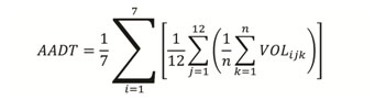
Where:
VOL = daily traffic for day k, of DOWi, and month j
i = day of the week
j = month of the year
k = 1 when the day is the first occurrence of that day of the week in a month, 4 when it is the fourth day of the week
n = the number of days of that day of the week during that month (usually between one and five, depending on the number of missing data)
AADTT – Annual Average Daily Truck Traffic – The total volume of truck traffic on a highway segment for one year, divided by the number of days in the year. Computation of AADTT (by vehicle class) from a short duration count requires the application of one or more factors that account for differences in time-of-day, DOW, and seasonal truck traffic patterns.
AAWDT – Annual Average Weekday Traffic – The estimate of typical traffic during a weekday (Monday through Friday) calculated from data measured at continuous monitoring sites.
AVDT – Annual Vehicle Distance Traveled – The number of miles that vehicles are driven in one year. AVDT is one of the values used in the Federal apportionment formula, and is calculated in distance units reported in HPMS for the roadway segment, usually in miles. This definition was added for accommodating distance measurements in the metric system.
The annual vehicle distance traveled (AVDT) is computed by multiplying the daily vehicle distance traveled (DVDT) by the number of days in the year. The HPMS software calculates the DVDT, and the AVDT is computed manually by FHWA.
The DVDT is calculated by multiplying the section AADT by the section length to compute section-specific DVDT. (A roadway section or subsection is a State-owned or off-system roadway identified by an eight-digit code. Each roadway section is defined by a beginning and ending milepost in the Roadway Characteristics Inventory (RCI)). These are then summed for an entire stratum to compute DVDT. Aggregate estimates at any stratification level (volume group, functional class, area type, statewide, or other combinations of these) can be derived by summing the DVDT of the appropriate strata. For example, to obtain estimates of rural interstate DVDT, sum the DVDT estimates for each volume group strata within the rural interstate functional system group.
Estimates of DVDT or AVDT for specific HPMS vehicle classes also can be derived by multiplying DVDT strata figures by the appropriate percentages derived from the vehicle classification counts and aggregating to the strata totals as done for volume.
An estimate of the standard error of a stratum DVDT estimate is given by the following equation:
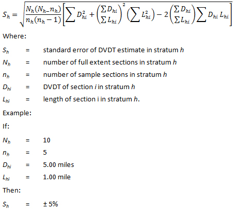
This equation is presented in Sampling Techniques (Cochran). A complete discussion of ratio estimation procedures is included in the reference. The estimates produced by this process are conservative since the errors introduced by using factors to develop AADT estimates have been ignored. The assumption is that these errors are normally distributed and therefore will cancel out when aggregated. The equation shows that estimates of the standard error of aggregate VDT for HPMS strata are derived by summing the squared standard errors of the appropriate strata and taking the square root of the total. Coefficients of variation and confidence intervals can be derived by standard statistical procedures.
As a rule of thumb, the precision of statewide DVDT estimates (excluding local functional class) is expected to approximate ±5 percent with 95 percent confidence, although the analysis assumed that the AADT values reported were exact. Because of this assumption, precision estimates are conservative. Computation of annual DVDT estimates with the complete HPMS standard sample by using the AADT from each HPMS standard sample would be expected to approximate the stated precision. It is important to note that precision and accuracy are different concepts from variability. For example, you can have variable traffic volumes from year-to-year but still have accurate volumes.
The HPMS standard sample sizes are defined in terms of AADT within strata (described in the HPMS Field Manual). To estimate the precision of DVDT estimates, a complex procedure is needed to account for the variation in AADT and for the variation in section length. The equation to estimate the sampling variability of aggregate DVDT estimates is given in Sampling Techniques. In an early HPMS study, the precision of statewide estimates of interstate DVDT approximated ±2-3 percent with 95 percent confidence, but these results considered only sampling variability and ignored error introduced by equipment or the factoring process used to estimate sample section AADT.
MADT – Monthly Average Daily Traffic – This can be computed by adding the daily volumes during any given month and dividing by the number of days in the month. For MADT, most of the calendar month of data should be included with a minimum of at least one Monday, Tuesday, Wednesday, Thursday, Friday, Saturday and Sunday.
MAWDT – Monthly Average Weekday Daily Traffic – The MADT for Monday through Friday are summed and then divided by five.
MAWET – Monthly Average Weekend Daily Traffic – The MADT for Saturday and Sunday are summed and then divided by two.
VDT – Vehicle Distance Traveled – The distance traveled by all vehicles for a given period, usually measured in miles and reported as vehicle miles traveled (VMT) for a geographic region. There is a relationship between VDT and VMT, although each is distinctly different. While VDT is measuring a distance traveled, VMT is counting the number of vehicles traveled over a distance. Depending upon the formulas used, these numbers may be the same.
VMT – Vehicle Miles Traveled – Indicates how many vehicles have traveled over the distance of a route or functional classification or geographic area in one day. VMT is calculated by multiplying the AADT value for each section of road by the section length (in miles) and summing all sections to obtain VMT for a complete route. VMT is not the same as daily vehicle distance traveled (DVDT), which measures the distance traveled by vehicles in a day, not how many (VMT) vehicles traveled over a given distance in a day. Depending upon the formulas used, these numbers may be the same.
Vehicle – Vehicles include one powered unit and may include one or more unpowered full-trailer or semi-trailer units (ASTM E17.52).
Vehicle Length – This refers to the overall length of a vehicle measured from the front bumper to the rear bumper including permanent equipment that may extend beyond the rear bumper such as that used to improve aerodynamic performance.
Vehicle Axle – The vehicle axle is the axis oriented transversely to the nominal direction of vehicle motion and extending the full width of the vehicle about which the wheel(s) at both ends rotate (ASTM E17.52, E1318-09).
Axle Spacing – For each vehicle axle, the horizontal distance between the center of that axle and that of the preceding axle is the vehicle axle spacing (ASTM E17.52, E1572-93).
Vehicle counting is the activity of measuring and recording traffic characteristics such as vehicle volume, classification, speed, weight, or a combination of these characteristics (ASTM E17.52, E1442-94).
Speed (Vehicle) – Measurement of how fast a vehicle is traveling in miles/hour (mph).
Weigh In Motion – Gross-vehicle weight of a highway vehicle is due only to the local force of gravity acting upon the composite mass of all connected vehicle components, and is distributed among the tires of the vehicle through connectors such as springs, motion dampers, and hinges. Highway WIM systems are capable of estimating the gross weight of a vehicle as well as the portion of this weight, called load, that is carried by the tires of each wheel assembly, axle, and axle group on the vehicle.
The FHWA vehicle classification system separates vehicles into categories depending on whether they carry passengers or commodities. Non-passenger vehicles are further subdivided by the number of axles and the number of units, including both power and trailer units. Note that the addition of a light trailer to a vehicle does not change the classification of the vehicle.
Axle-based automatic vehicle classifiers rely on an algorithm to interpret axle spacing information and correctly classify vehicles into these classes. The FHWA does not endorse any specific algorithm or system for interpreting axle spacings. Axle spacing characteristics for different vehicle classes are known to change from State to State, by region of the country. As a result, no single algorithm is best for all cases. It is the responsibility of each agency to develop, test and calibrate the classification algorithm they use. FHWA vehicle classes with definitions are identified in Appendix C of the TMG.
This section reviews the theory of vehicle detection, including the physics and electronics used with the various types of sensors.
The theory and operation of vehicle sensors is discussed in detail in the sensor technology chapter of the Traffic Detector Handbook (FHWA-HRT-06-108). The handbook also discusses the operation and uses of the following types of modern vehicle presence technologies:
With infrared sensors, the word “detector” takes on another meaning, namely the infrared sensitive element that converts the reflected and emitted energy into electrical signals. Real-time signal processing is used to analyze the signals for the presence of a vehicle. The sensors are mounted overhead to view approaching or departing traffic. They can also be mounted in a side-looking configuration. Infrared sensors are used for signal control; volume, speed, and class measurement; detection of pedestrians in crosswalks; and transmission of traffic information to motorists.
Table 1-2 describes the strengths and weaknesses of the types of technology used for presence detection. Presence detection refers to the ability of a vehicle detector to sense that a vehicle, whether moving or stopped, has appeared in its zone of detection.
| Technology | Strengths | Weaknesses |
|---|---|---|
| Inductive loop |
|
|
| Piezo/Quartz |
|
|
| Air switch/ Road tube |
|
|
| Magnetometer (two-axis fluxgate magnetometer) |
|
|
| Magnetic (induction or search coil magnetometer) |
|
|
| Microwave radar |
|
|
| Microwave doppler |
|
|
| Active infrared (laser radar) |
|
|
| Passive infrared |
|
|
| Ultrasonic |
|
|
| Acoustic |
|
|
| Video detection system |
|
|
Source: Adapted from Traffic Detector Handbook, 2006.
The Traffic Detector Handbook summarizes the comparison of in-roadway and over-roadway sensors and indicates that good performance of in-roadway sensors such as inductive loops, magnetic, and magnetometer sensors is based, in part, on their close location to the vehicle. Thus, in-road sensors are insensitive to inclement weather due to a high signal-to-noise ratio. Their main disadvantage is their in-roadway installation, necessitating physical changes in the roadway as part of the installation process. Over-roadway sensors often provide data not available from in-roadway sensors and some can monitor multiple lanes with one unit.
In traffic monitoring applications, in-road sensors can effectively discriminate vehicle characteristics (e.g. axle spacing, class, length) on a lane by lane basis, without being subject to errors introduced by multiple vehicles simultaneously in the field of view of the sensor.
The following table adapted from the Traffic Detector Handbook lists and describes the traffic flow sensor technologies and their capabilities. Most measure count, presence, and occupancy. Some single detection zone sensors, such as the range-measuring ultrasonic sensor and some infrared sensors do not measure speed. Continuous wave Doppler radar sensors do not detect stopped or slow moving vehicles.
| Sensor Technology |
Count | Presence | Speed | Output Data |
Classification1 | Multiple Lane, Multiple Detection Zone Data |
Communication Bandwidth |
Sensor Purchase Cost |
|---|---|---|---|---|---|---|---|---|
| Inductive Loop | X | X | Xa | X | Xb | Low to moderate | Lowh | |
| Magnetometer (2-Axis Fluxgate) |
X | X | Xa | X | Low | Moderateh | ||
| Magnetic Induction Coil | X | Xc | Xa | X | Low | Low to moderateh | ||
| Microwave Doppler | ||||||||
| Microwave Radar | X | Xd | X | Xd | Xd | Xd | Moderate | Low to moderate |
| Active Infrared | X | X | Xe | X | X | X | Low to moderate | Moderate to high |
| Passive Infrared | X | X | Xe | X | Low to moderate | Low to moderate | ||
| Ultrasonic | X | X | X | Low | Low to moderate | |||
| Acoustic Array | X | X | X | X | Xf | Low to moderate | Moderate | |
| Video Detection System | X | X | X | X | X | X | Low to highg | Moderate to high |
Source: Federal Highway Administration.
This section describes the kinds of technologies that are available to support traffic monitoring programs at the State level, including the technology and equipment used for collecting counts and the general strengths and weaknesses of each of those technologies. This section summarizes a large amount of previously published material and acknowledges that additional literature continues to be published as vendors bring new technologies to market and update existing technologies. An additional excellent source of information on the selection of traffic monitoring equipment can be found in Chapter 3 of the report AASHTO Guidelines for Traffic Data Programs (2009).
Traffic monitoring technology is evolving quickly due to a combination of the availability of modern, low cost computing and communications technology, but is also driven by the need for more timely information. Not all equipment vendors produce equipment of equal quality. Some equipment has been heavily tested and operates very robustly. Even within a single technology, equipment performance can vary widely from vendor to vendor based on each vendor’s internal software algorithms and the components that make up their equipment.
The reason different vendor’s equipment can produce different results for any given sensor technology is that the data collection electronics and the software that resides in those electronics may perform in different ways. (For example, two different video image-counting devices may produce very different results if one uses a robust image-processing algorithm, while the other does not.)
Consequently, as agencies make decisions on what type of hardware and supporting software to purchase, they should continue to consult the available and more detailed literature (such as from pooled funds, FHWA Highway Community Exchange, and FHWA Long Term Pavement Performance (LTPP)) that describes the performance of specific technologies. They should work cooperatively with their peers to share their working experience with specific equipment. Using these resources effectively is a key to selecting the best data monitoring equipment for each agency’s needs. A very good source of additional information on traffic data collection technologies is available on the FHWA’s Travel Monitoring Policy website. A variety of other excellent technical resources are included in Appendix L.
It is also important that agencies carefully test equipment before they purchase specific devices from a vendor, and once they have purchased devices that meet their needs, they should routinely calibrate and continue to test the performance of their equipment in the field. The first of these steps ensures that the equipment they purchase performs as advertised. The second step ensures that the equipment they are using is being correctly installed in the field, and that the performance of the sensors and electronics has not degraded over time due to use and changing environmental conditions. Careful site selection, use of high quality materials, and rigorous attention to detail during the installation process will facilitate the reliable collection of high quality traffic data on a continuous basis.
A good way to categorize traffic monitoring devices is based on the type of data they collect. Given the goals of the Traffic Monitoring Guide, traffic monitoring equipment can be categorized as being able to collect several different types of data:
The technology used to sense the passing traffic stream determines what each data collection device physically counts. The electronics connected to that sensor interpret the sensor’s signal, processes the signal (usually using a proprietary algorithm specific to that equipment’s vendor), and produces some subset of the data items listed in the bullets above. The next paragraphs describe the different types of data that are collected by traffic data collection equipment.
Chapter 4 provides basic guidance related to the state of the practice in non-motorized traffic monitoring. It includes discussion of the following:
Vehicle Volume
A wide variety of technologies can count vehicles. Some technologies actually count each passing object, where in most cases an object is a vehicle, whether it is a car or multi-unit truck. Other sensors do not detect a vehicle, but instead count the axles of those vehicles. Additional information is then used to convert the axle count data into measures of vehicle volume. In many cases, this extra information comes from a second sensor. But for simple, single sensor, axle-based counters, an adjustment factor (the axle correction factor) is applied against the total axle count in order to provide an estimate of vehicle volume. Table 1-4 summarizes which of the currently available traffic monitoring technologies directly count vehicle volumes, and which count axles requiring conversion of that data to vehicle volume estimates.
| Presence Sensing Technologies | Axle Sensing Technologies |
|---|---|
| Inductive loops | Infrared |
| Magnetic | Laser (most) |
| Video detection system | Piezo-electric |
| Acoustic | Quartz sensor |
| Ultrasonic | Fiber optic |
| Microwave radar | Capacitance mats |
| Laser radar | Bending plates |
| Passive infrared | Load cells |
| Inductive Signatures | |
| Contact switch closures (e.g., road tubes) |
This table shows the most common application of this technology. In some cases, specific implementations of the technologies can be used in different ways. For example, one very specific implementation of loop sensors has been shown to be able to count axles very accurately. However, most loop installations are not capable of detecting axles.
Collecting traffic volume data by vehicle classification differs from simple volume counting in that each vehicle is not only recognized as a vehicle, but that vehicle is also classified into one of several defined categories. Adding to the difficulty of categorizing vehicles is the fact that different users have different definitions into which they would like vehicles classified. In traffic monitoring, the most commonly used vehicle classification system is the 13 vehicle category classification system developed by FHWA and is used in each State’s HPMS submittal. Figure 1-1 provides representative examples that depict the 13 vehicle categories
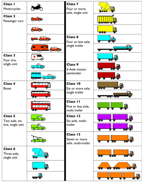
Source: Federal Highway Administration.
Certain truck configurations utilize axles that can be lifted when the vehicle is empty or lightly-loaded. The position of these axles—sometimes called lift axles, drop axles, or tag axles—affects the classification category into which the vehicle falls. To maintain consistency between visual and axle-based counts, the TMG recommends that only axles that are in the dropped position be considered when classifying the vehicle. While this promotes consistency, it may induce difficulty when interpreting summary classification statistics at certain locations. For example, a site may exhibit directional differences in vehicle classification even though the same trucks may be travelling one direction loaded (with axles down) and the other direction empty (with axles lifted).
This recommendation was developed as a compromise between a wide variety of competing interests. It is really a visual system. Most vehicles can be easily classified into this system by a human observer. However, work performed by John Wyman and others at Maine DOT (Wyman, Gary, and Stevens, 1985) resulted in computer algorithms that allow most vehicles to be correctly classified into these categories based on the number and spacing of their axles. This system has been refined over time by a wide variety of researchers, State agencies, and vendors to help it function effectively in their respective States. These modifications from the original system were necessary because truck size and weight laws vary from State to State and, consequently, common truck dimensions and configurations can change slightly from State to State. In addition, some States permit specific vehicle types that are not legal in other States. (For example, some western States allow tractors to pull three trailers, while most States do not allow more than two trailers.) States often wish to track these unusual vehicle types, and therefore add additional vehicle categories to FHWA’s 13 categories that meet their specific traffic monitoring needs. When these States purchase vehicle classification counters, they require that the vendors install their State-specific classification algorithms in the data collection electronics or post processing software.
However, these modified FHWA classification systems are not the only classification systems of interest. Many engineering and planning analyses do not require data in the detailed FHWA 13 categories, but do require information on truck volumes versus car volumes. Thus, many engineering and planning analyses use either a simple car/truck split or they use a very simplified truck classification system; commonly a 3- or 4-bin classification system based on vehicle length.
The most common length classification systems essentially consist of four generalized length bins that approximate the following four categories of vehicles: cars, small trucks, large trucks, and multi-trailer trucks. States that use only three truck classes combine the large truck and multi-trailer truck classes. (These States tend to be States where multi-trailer trucks are rare.) Unfortunately, unlike the FHWA 13 vehicle category classification, there is no common definition across the States that indicates the vehicle length at which a car becomes a truck. The States, therefore, set their own length definitions for these classification systems.
Besides its simplicity, one advantage of the length classification systems is that vehicle length can be easily calculated by a number of sensor technologies that do not require axle sensors. Thus, many of the sensor technologies that can collect volumes by vehicle length can be placed above or beside the roadway, limiting or eliminating the need for staff placing those sensors to work in the lane of travel.
The primary disadvantage of the length-based classification is that they do not correlate as well as the FHWA 13 vehicle category classification system to several of the key vehicle attributes used in specific types of analyses. For example, a major input to pavement design is traffic load, and that in turn is driven by the number and weight of axle loads being applied. The FHWA 13 vehicle category classification system directly accounts for the number of axles within the classification system. The FHWA classification system also does a good job of identifying specific vehicle types (e.g., classes 7 and 10) that are often particularly heavy. This results in better traffic load estimation and thus better pavement analysis.
Jurisdictions should adopt classification systems that are compatible with the 13 vehicle category classification system. Systems with fewer categories should be combinations of the FHWA classes, and systems with more categories should be subdivisions of the FHWA classes.
Length-based classification systems do not account for specific axle configurations, and thus the connection between the number and weight of axles within the different length classifications is far more nebulous. Similarly, the FHWA axle-based system does a good job of differentiating the number of multi-unit vehicles on the roadway, while the length-based systems are not able to track the number of vehicles pulling one or more other units. The number of units in a given vehicle is a key variable being tracked for safety purposes, thus the length classification systems are much less useful for the kinds of safety analyses that are interested in the exposure rates associated with multi-unit vehicles
Some State agencies use some combination of both FHWA’s 13 vehicle category classification system and a simpler length-based system. The length-based system is used in those physical road segments where it is not possible to place axle sensors. Length-based is also used when the advantages of simplicity outweigh the loss of detail and precision that comes from using the more sophisticated axle-based classification system. Approval is required by a State’s FHWA office for use of length class in any data submitted to FHWA
Table 1-5 describes which vehicle counting technologies can also classify vehicles.
| Technologies for Axle-Based Vehicle Classification |
Technologies for Length-Based Vehicle Classification |
|---|---|
| Infrared (passive) | Dual inductive loops |
| Laser radar | Inductive loops (loop signature) |
| Piezo-electric | Magnetic (magnetometer) |
| Quartz sensor | Video detection system |
| Fiber optic | Microwave radar |
| Inductive Loop Signatures | CW Doppler sensors |
| Capacitance mats | |
| Bending plates | |
| Load cells | |
| Contact switch closures (e.g., road tubes) | |
| Specialized inductive loop systems | |
| Any of the above combined with inductive loops |
Vehicle speed is also a commonly desired traffic monitoring attribute. Interest in monitoring and reporting roadway performance is growing at the State and Federal levels. This means that States are being asked to collect and report on where, how often, for how long, and to what extent roads are becoming congested. At the same time, safety and environmental studies are interested in the relative distribution of vehicle speeds, and the number and type of vehicles that are speeding.
Most modern traffic monitoring technologies produce a measure of speed as part of their routine traffic monitoring function. Roadway agencies are well advised to consider collecting and reporting speed data that can be used by their agency.
The selection of equipment to collect speed data should consider the fact that some technologies are particularly well suited for reporting individual vehicle speeds (that is tracking how fast each specific vehicle is moving), while others are designed to provide average facility speed over a given reporting interval. Although both data represent speed information, the usefulness of those data is very different
How the speed data is collected is as much a function of the equipment connected to the sensor as it is of the sensor technology itself. For example, the traditional method for estimating speeds when using a single inductive loop is to measure total sensor on time (lane occupancy) over a set period, along with the total number of vehicle observations during that period. By dividing the lane occupancy by the volume and multiplying by a constant that represents the average vehicle length for that location, average speed for that reporting period can be computed and reported. However, more modern electronics can take the same basic single loop signal, and by analyzing that signal, directly calculate vehicle speed from the shape of the loop signature. Another approach to using loop technology is to place two loops in the lane at a known distance apart configured one after the other, thus forming a speed trap. When these loops are properly calibrated, the distance between the leading edge of the two detectors (d12) divided by the difference in time it takes for the passing vehicle to activate the second loop after it activates the first loop (T2 – T1) yields the speed of the vehicle (d12 / (T2 – T1)).
The key to collecting speed data is that the agency needs to understand both what use they need from the data, and what their available equipment can supply.
Speed data can also be obtained from other sources. One such source is vehicle probe data; however, guidance on how to combine speed data collected from vehicle probes within the overall roadway performance-monitoring program of an agency is not covered in this edition of the TMG. FHWA now has a speed format that allows for flexibility with a minimum of 15 speed bins to a maximum of 25 speed bins (all in 5 mph increments).
The final traffic attributes that should be addressed as part of a traffic monitoring program is axle weights and spacings. A specific subset of traffic monitoring devices is capable of weighing vehicles while they travel down the road. These devices are commonly referred to as weigh-in-motion (WIM) scales. The sensors used are designed to not only detect the presence of an axle, but to measure the force being applied by that axle during the duration of the time the axle is in contact with the axle sensor. Sophisticated analysis is then applied to the signal produced by each sensor in order to establish the weight of each passing axle. Weights for all axles associated with a given vehicle are then combined to estimate total vehicle weight. Axle spacings are also recorded.
The most common of WIM technologies used in the U.S. are piezo-electric and bending plate systems. There are a variety of different piezo-electric and quartz sensor technologies, each of which has specific strengths and weaknesses. In addition, other technologies such as fiber optic cables, load cells (both hydraulic and mechanical), capacitance mats, and strips, along with bridges and culverts instrumented with strain gauges can also be used as weight sensors.
In almost all cases, secondary sensors (e.g., inductive loop detectors) are used in combination with the primary axle and weight sensors to provide information on presence. Combining vehicle speed and presence information with the time between axle weight measurements allows the WIM system to correctly assign specific axles to specific vehicles and to group the axles correctly (that is, are the observed axles single axles, tandem axles, tridems, or even larger groups of axles), and thus correctly classify each vehicle and compute its total weight. It is important to note that WIM measures the dynamic axle weights, and these are different from static axle weights.
The relatively small amount of metal in many motorcycles combined with the fact that many motorcyclists ride near lane lines in order to give themselves more time to avoid cars moving into their lanes means that inductive loop detectors and half lane axle sensors often undercount motorcycles. When motorcycles ride in closely spaced groups, the closely spaced axles and cycles often confuse available traffic monitoring equipment, which have not been designed to identify the resulting pattern of closely spaced axles and vehicles. Guidance for how to address these issues is included in Chapter 3.
For much of the 20th century, most traffic monitoring devices were placed on top of or in the pavement (e.g., road tubes versus inductive loops). These sensors are commonly referred to as “intrusive” sensors. Micro loops are placed in a tube below the ground (shuttle).
As traffic volumes have grown over time, it has become both increasingly difficult and costly to quickly and safely place sensors on, or in, the travel lane. The most common reasons for not wanting to place sensors in or on the lane of travel are as follows:
As a result, considerable work has been done during the last 20 plus years to bring to market non-intrusive sensors that can be put in place and/or maintained without personnel having to enter the travel lane. Table 1-6 describes which sensors are intrusive and which are non-intrusive.
| Intrusive | Non-Intrusive |
|---|---|
| Inductive loops | Infrared (passive) |
| Piezo-electric | Video detection system |
| Quartz sensor | Microwave radar (overhead or side mounted) |
| Fiber optic | CW Doppler sensor |
| Magnetic (most sensor designs) | Acoustic |
| Contact closures | Ultrasonic |
| WIM scales (bending plates, load cells, capacitance mats and strips) | Laser radar |
Non-intrusive sensors can be further divided into overhead mounted sensors and side-fired sensors. Side-fired sensors have the advantage of being mounted beside the road. This makes them easy to install, access, and maintain. The drawback is that on multi-lane roadways, traffic using the roadway lanes farthest away from the sensor location can be obscured from the side-fired sensors by vehicles (and particularly trucks) traveling in the lanes closer to the sensor. This is called occlusion. Occlusion results in undercounting of total volume and can bias speed estimates if the traffic on the inside of the roadway is traveling at a different speed than traffic on the outside lanes.
Generally, the higher above the roadway the non-intrusive sensor is placed, the smaller the problem with occlusion. However, raising the sensor vertically can 1) increase the cost of installation and maintenance; 2) decrease the resolution with which the sensor detects vehicles in the road; and 3) create movement in the sensor (as the pole on which the sensor sits sways), which may result in other forms of accuracy degradation.
Mounting the sensor directly above the lane of travel is one way of significantly reducing the opportunity for occlusion to occur. Thus, overhead mounted sensors tend to be more accurate than side-fired sensors of that same technology. The disadvantage of overhead mounted sensors is that the lane of travel must normally be shut down in order for the sensors to be installed and then again each time maintenance is performed because of fears that material could be dropped onto the roadway during those activities. This can be problematic for some high volume roadways. Axle weights are the one form of data that cannot be collected non-intrusively. (Some bridge WIM systems are designed to operate without sensors being placed in the lane of travel. But to date, these systems only work on a very limited set of bridges and are still primarily in the research phase.)
In addition to the basic functional requirements discussed above, roadway agencies should consider a variety of other functionalities when selecting traffic monitoring technologies. These topics include:
14. Number of lanes of data collection performed by any one piece of equipment and/or sensor;
15. Cost of the equipment (initial cost, placement cost, operating cost, and expected maintenance costs);
16. Expected life of the sensors and data collection electronics;
17. Warranties supplied by the manufacturer/vendor;
18.Environmental conditions under which the equipment is expected to operate relative to the strengths and weaknesses of each specific technology;
19. Whether the agency staff has the required knowledge and equipment for placing, calibrating, and maintaining the equipment;
20. Available communications capabilities (i.e., what options does the agency have for retrieving data from the data collection electronics, and how do those options fit within the agency’s current or planned traffic data processing procedures?);
21. Type of power source to be used (AC/DC, solar, luminary, internal battery);
22. Ability of the vendor to supply data outputs in a format that works seamlessly with the agency’s existing or planned data processing system (ability to integrate data into a centralized system and utilize information to calculate and summarize statewide year-end statistics);
23. Vendor agreement for software support, equipment maintenance, warranty work;
24. Pavement condition for surface sensor like piezos and WIM; and
25.Installation materials and methods
The first four of these issues are straightforward and provide the reviewer with the ability to trade-off cost and performance. Of particular importance is the warranty provided by the vendor, as it provides an important level of assurance that the first three cost estimates are accurate.
The fifth topic relates to the fact that some technologies work better in some specific environmental and traffic conditions than others. Some equipment might work very well in specific instances while work poorly in other circumstances. For example, road tubes generally work well for short duration counts (48 hours) on lower volume, rural roadways. However, they do not work effectively on higher volume, multi-lane urban roadways. While vendors can create product modifications/versions to help technologies function in conditions for which they are generally not suited, when selecting technologies, agencies should be very aware of the increased likelihood of count issues/failures from those technologies in those conditions.
The answer to the sixth topic determines whether the agency needs to purchase additional equipment to place, operate, and maintain new technologies, as well as have staff undergo new training in order to perform those tasks.
Finally, the last six topics describe how efficiently and reliably the vendor’s implementation of the selected technology will work within the existing or planned data processing system of the roadway agency. Collection, calibration, processing, reporting, accessing, and storing of traffic monitoring data can be resource intensive and roadway agencies should consider how much effort would be required for any given device.
Regardless of the traffic monitoring technology selected, every roadway agency should routinely perform the following tasks to ensure that the equipment they purchase works to the best of its capability:
These tasks, described in more detail in Chapters 2 and 3, ensure active management from those collecting and using the data so that the technology performs well.
Equipment that is not actively monitored for quality performance eventually goes out of calibration, regardless of a vendor’s assurances of self-calibration capabilities. Validation checks when equipment is initially installed are an essential first step in that process. Following a formal quality assurance and field maintenance program and providing resources to fix problems that are identified by that process ensures that funding available for collecting data is spent on collecting valid, useful information.
The next section describes the concepts regarding variability in traffic patterns, which should be considered when establishing traffic data collection programs.
This section discusses the concepts of different types of variability found in traffic patterns and describes how this variability affects the design of a strong traffic monitoring program. Traffic volumes typically vary over time and space. That is, traffic volumes are different at 8 a.m. than they are at 8 p.m. Similarly, traffic patterns are different on urban freeways and on rural farm to market roads. A good traffic monitoring program collects data to meet many needs; therefore, a roadway agency should design data collection efforts that provide the roadway agency with an accurate understanding of exactly what these patterns are and how they are changing over time.
The next paragraphs introduce the concepts of traffic variability and describe the program and technology designs that are used to account for this variability.
Technology allows agencies to collect enough data to accurately describe how traffic varies over time and space (Wright et al., 1997). Traffic varies over a number of different time scales, including:
Traffic varies from place to place and directionally too. Not only do roads carry different volumes of traffic, but also the characteristics of the vehicles using those roads change from facility to facility. One road with 5,000 vehicles per day may have very little truck traffic, while another road with the same volume of vehicles may have 1,000 trucks per day mixed in with 4,000 cars. Similarly, one road section may be traversed by 1,000 heavily loaded trucks per day while a nearby road is used by 1,000 partially loaded trucks. Directional variations also exist.
Since the early development of roads, it has been known that the use of a road changes during the course of the day. In most locations, traffic volumes increase during the day and decrease at night. A 1997 study for the Federal Highway Administration (Hallenbeck, et al., 1997) determined that most truck travel falls into one of two basic time-of-day patterns; one pattern is centered on travel during the business day, and the other pattern shows almost constant travel throughout the twenty-four-hour day.
Most passenger car travel also falls into one of two time-of-day patterns, but these patterns are different from those of trucks. These four patterns are illustrated in Figure 1-2.
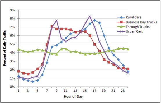
Source: Hallenbeck, et al., Vehicle Volume Distributions by Classification, 1997.
As can be seen in Figure 1-2, cars tend to follow either the traditional two-humped urban commute pattern or the single-hump pattern commonly seen in rural areas, where traffic volumes continue to grow throughout the day until they begin to taper off in the evening. Trucks also exhibit a single mode. However, the truck pattern differs from the rural car pattern in that it peaks in the early morning (many trucks make deliveries early in the morning to help prepare businesses for the coming workday) and tapers off gradually, until early afternoon, when it declines quickly. The other truck pattern (travel constantly occurring throughout the day) is common with long haul trucking movements.
The traffic at any given site comprises some combination of these types of movements. In addition, at any specific location, time-of-day patterns may differ significantly as a result of local trip generation patterns that differ from the norm. For example, Las Vegas, Nevada, generates an abnormal amount of traffic during the night because that city is very active late at night. In heavily congested urban areas, the commute period traffic volume peaks flatten out and can last three or more hours. Local patterns also have a significant effect on the directional time-of-day pattern for any given road. On some urban roadways, there is very heavy directional traffic movement – inbound to the central city in the morning and outbound to the suburbs in the afternoon. On other roadways, especially freeways serving multiple suburban cities, traffic can be equally strong in both directions during both commute periods.
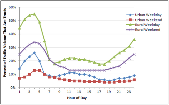
Because the volumes of cars and trucks are very different from one site to another, the effect of these different time-of-day patterns on summary statistics such as percent trucks, percent bicycles, percent pedestrians, and total volume can be unexpected. Often, in daylight hours, car volumes are so high in comparison to truck volumes that the car travel pattern dominates and the percentage of trucks is very low. However, at night on that same roadway, car volumes may decrease significantly while through-truck movements continue so that the truck percentage increases considerably and total volume declines less than the car pattern would predict. Figure 1-3 shows how typical values of truck percentages change during the day for urban and rural settings on both weekdays and weekends.
Because these changes can be so significant, it is important to account for them in the design and execution of the traffic monitoring program as well as in the computation and reporting of summary statistics.
Source: Hallenbeck, et al., Vehicle Volume Distributions by Classification, 1997.
Time-of-day patterns are not the only way car and truck patterns differ. DOW patterns also differ in large part because of the use of cars for a variety of non-business related traffic, whereas for the most part, trucks travel only when business needs require.
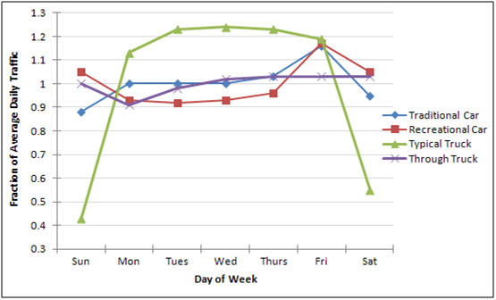
Similar to the time-of-day patterns, DOW patterns for cars fall into one of two basic patterns as shown in Figure 1-4. In the first pattern (traditional urban), volumes are fairly constant during weekdays and then decline slightly on the weekends, with Sunday volumes usually being lower than Saturday volumes. This pattern also exists on many rural roads. The alternate pattern, usually found on roads that contain recreational travel, shows constant weekday volumes followed by an increase in traffic on the weekends.
Source: Hallenbeck, et al., Vehicle Volume Distributions by Classification, 1997.
Trucks also have two patterns that are both driven by the needs of businesses. Most trucks follow an exaggerated version of the traditional urban car pattern. That is, weekday truck volumes are constant, but on weekends, truck volumes decline considerably more than car volumes (unlike cars, the decline in truck travel caused by lower weekend business activity is usually not balanced by an increase in truck travel for other purposes). However, as with the time-of-day pattern, long haul through trucks often show a very different DOW pattern. Since long-haul trucks are not concerned with the business day (they travel as often as the driver is allowed), they travel equally on all seven days of the week. Thus, roads with high percentages of through-truck traffic often maintain high truck volumes during the weekends, even though the local truck traffic declines. Note that through-truck traffic is still normally generated during normal business hours. Thus, through-traffic generated from any one geographic location has the same 5-day on, 2-day off pattern seen in the local truck pattern. Where a road carries through-truck traffic from a single dominant area, the two-day lag in truck volumes is often apparent. However, the lag appears at some other time in the week. This pattern is visible in truck volume counts only when through-truck traffic is a high percentage of total truck volume. What happens more commonly is that weekend truck volumes do not drop as precipitously as they do at sites where little through-truck traffic exists.
These significant changes in traffic volumes during the course of the week have several effects on the traffic monitoring program. Most importantly, the monitoring program should collect data that allow a State to describe these variations. Second, the monitoring program should allow this knowledge to be shared with the users of the traffic data and applied to individual locations. Without these two steps, many of the analyses performed with traffic monitoring data will be inaccurate. Pavement designers need to account for reductions in truck traffic on the weekends if they are to accurately predict annual loading rates. Likewise, accident rate comparisons for different vehicle classifications are not realistic unless these differences are accounted for in estimates of vehicle miles traveled by class.
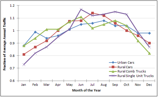
Further complicating the analysis of temporal variation in traffic patterns is the fact that both car and truck traffic change over the course of the year. Monthly changes in total volume have been tracked for many years with permanent counters, traditionally called Continuous Count Station. Total volume patterns from these devices show a variety of patterns, including common patterns such as the flat urban and rural summer peak shown in Figure 1-5.
Source: Hallenbeck, et al., Vehicle Volume Distributions by Classification, 1997.
Most States track four or more monthly patterns and they base the patterns being followed on some combination of functional classification of roadway and geographic location. Geography and functional classification are used as readily available surrogate measures that describe roads that follow that basic pattern. Geographic stratification is particularly important when different parts of a State experience very different travel behavior. For example, travel in areas that experience heavy recreational movements follow different travel patterns than those in areas without such movements. Even in urban areas where travel is more constant year round, cities with heavy recreational activity have different patterns than cities in the same State without heavy recreational movements.
Not surprisingly, truck traffic has monthly patterns that are different from automobile patterns. Some truck movements are stable throughout the year. These movements are often identified with specific types of trucks operating in specific corridors or regions. Other truck movements have high monthly variability, for example, in agricultural areas. It has even been shown that the weights carried by some trucks vary by season. This is particularly true in States where monthly load restrictions are placed on roads and where weight limits are increased during some winter months. Where this happens, States should track monthly changes for the development of adjustment factors.
As with day-of-week patterns, tracking of monthly changes in volumes is useful to calculate adjustments needed for various analyses. If annual statistics are needed for an analysis, it is necessary to adjust a short duration traffic volume count taken in mid-August to account for the fact that August traffic differs from the annual average condition.
Research has shown that monthly monitoring and adjustment should be done separately for trucks and cars (Hallenbeck, et al., 1997). Truck volume patterns can vary considerably from car volume patterns. Roads that carry significant volumes of through-trucks tend to have very different monthly patterns than roads that carry predominately local freight traffic. Roads that carry large volumes of recreational traffic often do not experience similarly large increases in truck traffic, but do often experience major increases in the number of recreational vehicles, which share many characteristics with trucks but have significant differences in weights.
Thus, it is highly recommended that States monitor and account for monthly variation in truck traffic directly, and that these procedures be independent of the procedures used to account for variations in car volume.
Most two-way roads exhibit differences in flow by direction by time of day. The traditional urban commute involves a heavy inbound movement in the morning and an outbound movement in the afternoon. On many suburban roads, this directional behavior has disappeared, replaced by heavy peak movements in both directions during both peak periods. When these directional movements are combined, the time-of-day pattern shown in Figure 1-2 is still evident, but when looked at separately, new time-of-day patterns become apparent.
In areas with high recreational traffic flows, directional movements change the DOW traffic patterns as much as the time-of-day patterns. Travelers often arrive in the area starting late Thursday night and depart on Sunday.
Truck volumes and characteristics can also change by direction. One example of directional differences in trucks is the movement of loaded trucks in one direction along a road, with a return movement of empty trucks. This is often the situation in regions where mineral resources are extracted. Volumes by vehicle classification can also change from one direction to another, for example when loaded logging trucks (classified as 5-axle tractor semi-trailers) move in one direction, and unloaded logging trucks (which carry the trailer dollies on the tractor and are classified as 3-axle single units) move in the other.
Tracking these directional movements as part of the statewide monitoring program is important for not only planning, design, and operation of existing roadways, but as an important supplement to the knowledge base needed to estimate the impacts that new development will generate in previously undeveloped rural lands.
The last type of variation discussed is spatial variation. That is, how volumes change from one roadway to another, or from one location on a road to another location on that same road. This type of differentiation is taken for granted for traffic volumes. Some roads simply carry more vehicles than others do. This concept is readily expanded to encompass the notion discussed above, that many of the basic traffic volume patterns are geographically affected (e.g., California ski areas have different travel patterns than California beach highways). It is important to extend these concepts even further to recognize that truck travel also varies from route to route and region to region. It is just as important to realize that differences in truck travel can occur irrespective of differences in automobile traffic
One important area of interest in traffic monitoring is the creation of truck flow maps and/or tonnage maps. These maps (analogous to traffic flow maps) show where truck and freight movements are heaviest. This is important for the following:
When these truck flow maps are developed, they often reveal that truck routes exist irrespective of the total traffic volume and/or the functional classification of the roads involved. Trucks use specific routes because those roads lead from the truck’s origin to their destination, and the route has sufficient geometric capacity to accommodate them. Truck drivers do not select a route because it is designated as a rural principal arterial. They select a route because of how it serves their route purposes. Consequently, functional classification is a very poor predictor of truck volume or percentage. As an example, interstates that serve major through truck movements (even in urban areas) tend to have high truck volumes, but interstates that do not service major freight movements tend to have low truck volumes. While both of these are functionally classified as interstates, they do not have the same truck flow characteristics
Because truck flows (both truck volumes and weights) play such an important (and growing) role in highway engineering functions, it is vital that States collect truck volume data that describe the geographic changes that exist. Which roads carry large freight movements? Which roads carry large truck volumes, even if those volumes are a small percentage of total traffic volume? Which roads restrict or carry light volumes of freight?
The variability described in the previous paragraphs should be measured and accounted for in the data collection and reporting program that a State designs and implements. The data collection program should also identify changes in these traffic patterns as they occur over time. To meet these needs in a cost effective manner, statewide traffic monitoring programs generally include:
The short duration counts provide the geographic coverage needed to understand traffic characteristics on individual roadways, as well as on specific segments of those roadways. They provide site-specific data on the time-of-day and DOW variation in travel, but are mostly intended to provide current general traffic volume information throughout the larger monitored roadway network. However, short duration counts cannot be directly used to provide many of the required data items desired by users. Statistics such as annual average traffic or design hourly volume cannot be accurately measured during a short duration count. Instead, data collected during short duration counts are factored or adjusted to create these estimates. The procedures to develop and apply these factors are discussed in Chapter 3 of the TMG.
To develop those factors, an agency should have a modest number of permanently operating traffic monitoring sites. Permanent data collection sites provide data on seasonal and day-of-week trends. Continuous count summaries also provide very precise measurements of changes in travel volumes and characteristics at a limited number of locations.
Importantly, while the basic traffic variables required for short- and permanent-duration counts is the same (i.e., volume, volume by class, speed, weights), these two types of data collection efforts place different demands on data collection technology, and thus the equipment well suited for short duration counts is not always well suited for permanent counting and vice-versa. The implications of these different types of data collection durations on equipment selection are discussed in the following sections.
The key to short duration counts is that they should be easy and inexpensive to perform, while the sensors should remain in place and function properly for the duration of the count. Because they are designed to give wide geographic coverage, most highway agencies typically perform a large number of short duration counts, each being performed at a new location. As a result, short count programs tend to be staff intensive, with the data collection staff working frequently within the roadway right-of-way to place and retrieve data collection sensors and equipment. This leads to two major priorities when selecting the appropriate technologies for performing short duration counts (in addition to the issues discussed in the previous paragraphs, and the accuracy and price of the equipment). Technologies used for short duration counts should:
Other attributes that are less dependent on sensor technology but also very important when selecting short duration count equipment include:
The speed of sensor placement and related equipment set up and calibration is important because staff usually perform a large number of short duration counts. As a result, considerable cost is involved in the placement and retrieval of equipment. The faster sensors and data collection equipment can be placed, the more count locations a given staff member can place in a day and the lower the cost of collecting that data. Nevertheless, at the same time, the placement (and pick up) of those sensors must not endanger the staff placing that equipment. This need to safeguard data collection staff, without having to go to the cost of applying full-scale traffic control, is one of the reasons so much effort has been spent on exploring non-intrusive data collection technologies. However, on lower volume roads where low cost road-tube axle sensors can be easily placed, intrusive sensors are still commonly used.
Where intrusive sensors cannot be safely and easily placed, agencies either use non-intrusive sensors or accept the cost of substantial traffic control each time a sensor must be placed in the roadway. Where short counts are used routinely at such locations, but the agency is not interested in investing permanent equipment, another option is to place permanent intrusive sensors in the roadway but not to connect those sensors to permanent power and communications. Instead, to use these sensors, the agency simply connects portable data collection electronics to the sensor leads, which are stored in a weatherproof enclosure until they are needed again. This approach saves the agency both the initial capital expenditure of bringing power and communications to the site, and the cost of traffic control during subsequent site visits. However, this approach is only cost effective if the permanent sensors are long lived, and if that location is to be visited for data collection routinely.
If non-intrusive sensors are the desired option, U.S. DOT has worked with several State highway agencies to develop new ways of deploying modern non-intrusive traffic monitoring technologies for short duration counts (Kotzenmacher, Minge, and Hao, 2005). The most common of these approaches is to affix the non-intrusive sensors to an extendable pole, which is placed on a trailer. The trailer is then towed to the roadside locations, placed in a safe position behind a barrier, and the pole raised. The sensors are then calibrated and the entire trailer system left in place for the duration of the count.
Short counts are commonly made for all of the traffic attributes, including volume, volume by classification of vehicle (including bicycles), speed, and axle weights. (Note that axle weights can only be collected with a high degree of accuracy using intrusive technologies that cannot be put in place quickly (Hallenbeck and Weinblatt, 2004). This means that most roadway agencies collect axle weight data from permanent data collection sites.) Table 1-7 describes the sensor technologies that are commonly used for short duration counts and the motorized vehicle attributes they routinely collect.
| Technology | No. Sensors Needed for Speed Data Collection | Types of Vehicle Classifications Collected | Number of Lanes of Data Collected by Each Sensor | Environmental Issues/Concerns | Other Issues/Concerns |
|---|---|---|---|---|---|
| Road Tubes – traditional | 2 (One lane only) | Axle Based(FHWA 13+) | 1 per pair of sensors(Only lanes bordering shoulders) | Not suited to snowy conditions | Accuracy limitations under very heavy traffic volumes or stop-and-go conditions |
| Road Tubes – multi-lane design | 2 per lane | Axle Based(FHWA 13+) | 1 per pair of sensors | Not suited to snowy conditions | Accuracy limitations under very heavy traffic volumes or stop-and-go conditions |
| Tape Switches | 2 per lane | Axle Based(FHWA 13+) | 1 per pair of sensors | Placement difficulties in wet conditions | Needs protection of lead wires if placed on lanes not adjacent to shoulders |
| Magnetometer (several different variations on this technology exist) | 2 per lane | Length-Based (for most sensor designs) | 1 per sensor (2 sensors per lane if speed or vehicle length is needed) | Most magnetic technology sensors require a short lane closure for sensor placement | Some magnetic sensors are placed in the pavement, others on the pavement, and others under the pavement |
| Video Detection System | 1 camera | Length-Based | Multiple | Does not work well in snow, fog, or dust storms | Short duration counter is mounted on an extendible pole on a trailer pulled to the count site; generally slow to set up |
| Piezo-sensors (piezo-film, piezo-cable) | 2 per lane | Axle Based(FHWA 13+) | 1 per pair of sensors | Very cold weather may affect performance | Needs protection of lead wires if placed on lanes not adjacent to shoulders |
| Infrared | 1 (transmitter + receptor) | Axle Based(FHWA 13+) | Multiple | Fog and heavy snow can degrade performance and large crown in road will block beams; Occlusion | |
| Microwave radar | 1 per direction (side-fired), 1 per lane (overhead) | Length-Based | Multiple | Can have occlusion issues with heavy or stop-and-go traffic and multiple lanes | Short duration counter is mounted on an extensible pole on a trailer pulled to the count site |
| Acoustic | 1 sensor | None | Multiple | Background noise/sound may interfere | Short duration counter is mounted on an extensible pole on a trailer; the sensor should be mounted higher than 25 feet |
| Laser Radar | 1 sensor | 13+ | Maximum of 4 | Snow, fog, heavy rain | No in-road installation required |
Source: Hallenbeck and Weinblatt, 2004.
Permanent, continually operating traffic monitoring equipment is used to provide both current measures of traffic flow and to provide a time series record of traffic flow attributes that describe how traffic flow changes over time at that location. Permanent traffic monitoring locations should have:
Permanent sensors represent both a large financial investment and a large data resource. As a result, the selection, installation, and calibration of that equipment is particularly important. Sensors that are poorly installed, inadequately calibrated, or that fail quickly because of poor design or construction, not only do not generate useful data, they waste resources (both money and staff time) that are needed for other data collection tasks. In part, this is because the funds spent on equipment and installation could be used elsewhere, but also because it requires considerable staff time to determine that the data being provided by poorly performing sensors are not an accurate representation of the traffic stream.
Unlike short duration counts, the speed of sensor installation is much less of an issue for selecting permanent count technology and equipment. The real key for permanent count technologies is that once installed, the equipment should operate accurately for long periods, with only a modest level of maintenance. In high volume locations, maintenance of an intrusive sensor may not actually be possible unless lane closures are planned for some other purpose. (In a growing number of urban areas, traffic lane closures are very limited due to the size and scope of traffic congestion those closures cause, even at night.)
One of the great advantages of non-intrusive detectors as permanent traffic monitoring devices is the ability of the roadway agency to work on that equipment when it starts to have performance problems. Of course, not all non-intrusive equipment has this advantage, and in other instances, non-intrusive equipment can be placed either beside the roadway (fully accessible) or above the roadway (requiring lane closures for maintenance), but the side-fired equipment positions come with penalties to the accuracy with which the devices work.
Table 1-8 summarizes the technologies currently used for permanent vehicular traffic monitoring.
| Technology | Intrusive or Non-intrusive | Types of Vehicle Classifications Collected WIM? | Number of Lanes of Data Collected by Each Sensor | Environmental Issues/Concerns | Other Issues/Concerns |
|---|---|---|---|---|---|
| Piezo-Electric Cable | Intrusive | Axle Based(FHWA 13+) Can be used for WIM | 1 per pair of sensors | Susceptible to damage from mill and resurface and oversized trucks Susceptible to snowplow damage, if not flush with surface |
Temperature sensitive (for weight classification); doesn’t work well in stop-and-go traffic |
| Piezo-Polymer Film | Intrusive | Axle Based(FHWA 13+)Can be used for WIM | 1 per pair of sensors | Temperature sensitive (for weight classification); doesn’t work well in stop-and-go traffic | |
| Piezo-Quartz Cable | Intrusive | Axle Based(FHWA 13+)A good WIM sensor | 1 per set of sensors | Piezo-Quartz sensors are typically ½ lane in width, so a site may require 4 sensors/lane; it is possible to instrument only on wheel path, with modest loss of volume and classification accuracy | |
| Other Pressure Sensors | Intrusive | Axle Based(FHWA 13+) | 1 per pair of sensors | Doesn’t work well in stop-and-go traffic | |
| Inductive Loop (conventional) | Intrusive | Length-Based | 1 per pair of sensors | Freeze/thaw can break loops | Single loops can be used to collect volume and lane occupancy, from which speed can be estimated |
| Inductive Loop (undercarriage profile) | Intrusive | Variousa | 1 per set of sensors | New technology, not currently in widespread use | |
| Side-Mounted Microwave Radar | Non-intrusive | Length-Based | Multiple | Not as accurate as overhead-mounted, forward-, or rear-facing radar (getting close) | |
| Overhead Microwave Radar | Non-intrusive | Length-Based | 1 per sensor | ||
| Doppler Radar | Non-intrusive | None | Multiple | Generally used only for speed data collection, often not accurate as a volume counting device | |
| Infrared | Non-intrusive 1 (transmitter + receptor) | Axle Based(FHWA 13+) | Multiple | Fog and heavy snow can degrade performance | Most common device requires equipment on both sides of the right of way |
| Magnetometer(3-axis flux gate) | Intrusiveb | Length-Based | 1 per pair of sensors | ||
| Magnetometer(magnetic imaging) | Intrusive | Length-Based | 1 lane | ||
| Video Detection System(trip wire) | Non-intrusive | Length-Based | Multiple | Can be affected by heavy fog, snow, glare, dust | Requires proper mounting height |
| Video Detection System(object analysis) | Non-intrusive | Variousc | Multiple | Can be affected by heavy fog, snow, glare, dust | Requires proper mounting height; new technology, not currently in widespread use |
| Ultrasonic | Non-intrusive | Length-Based | 1 per pair of sensors | Temperature variation and air turbulence can affect accuracy | New technology, not currently in widespread use |
| Acoustic | Non-intrusive | None | 1 per pair of sensors | Must be carefully calibrated | |
| Bending Plate | Intrusive | Axle Based (FHWA 13+) A good WIM sensor | 1 per set of sensors | Too expensive unless used as a WIM scale | |
| Bridge WIM | Non-intrusive | Axle Based (FHWA 13+)a WIM scale | Only works on specific types and sizes of bridges and culverts; not really a conventional traffic monitoring device | ||
| Load Cell | Intrusive | FHWA 13+ | 1 per wheel path | Large upfront cost | Maintenance costs are yearly and require lane closure |
Source: Hallenbeck and Weinblatt, 2004.
a There are two basic undercarriage loop classifier technologies. One uses the “signature” from existing loops to determine classification by matching the shape of that loop to expected profiles. The other uses specific types of loops to detect changes in inductance associated with wheels, and uses that information to detect and measure axles. This device can classify by “axle,” while the other defines classes that relate strongly to axle-based classes but are not specifically based on the number and spacing of axles.
b Overhead-mounted, non-intrusive detectors require a structure (usually a bridge or gantry) upon which to be mounted. The expense of sensor installation increases dramatically where these do not already exist.
c Video image analysis will define classes based on the features the software can detect. The simplest detection algorithms are based on length. More complex algorithms can detect and classify using axle information, provided the camera angles are capable of “seeing” different axles.
This chapter discussed the theory, technology, and concepts that are used as the basis for developing a traffic monitoring program. The strengths and weaknesses of the various types of technology and equipment were also presented. The States should consider which combinations of technology and equipment best suit their needs when establishing their traffic data collection programs.

