Evaluation of State Quality Assurance Program Effectiveness

APPENDIX B

SPECIFICATION 2

Per FHWA request, appendix B was added to this report. This appendix is a repetition of the initial analysis of the HMA acceptance plan for specification 2 except that the thickness quality characteristic has been excluded, leaving only density and air voids. Appendix B was added because the specification is frequently applied without including thickness as part of the pay-adjustment acceptance procedure. Repetition was used to make it easier for readers to understand.

Acceptance Procedure Synopsis

Type of Specification

• HMA pavement.

Quality Characteristics

• Density (one-sided, field test).
• Air voids (two-sided, plant test).

Correlation of Quality Characteristics

• No information available; assume uncorrelated.

Lot Size Definitions

• Density:. Day’s production.
• Air voids:
• Four contiguous air tests taken at the plant.
• Acknowledged to be different from density lots.
• Applies to tonnage represented.

Sample Sizes

• Density, n = 10.
• Air voids, n = 4.

Statistical Quality Measure

• PWL.

Individual Pay Equations (PA as Decimal)

• Surface, base, and pavements.
• Density: Figure 103 is used to calculate the pay equation for density as follows:

Figure 103. Equation. Individual density pay equation for surface, base, and pavements.

Where:

• PA is applied to $40 per ton.
  
  
• Added or subtracted on pay estimate.
  
  
• AQL of PWL = 90 is implied since this produces PA = 0 at PWL = 90.
  
  
• If PWL < 50, agency will evaluate. If left in place, PA = -0.16 (calculated value for PWL = 50) unless a lower value is negotiated.
  
  
• RQL consequence is not specified in a form that can be analyzed by SPECRISK.

• Air voids: Figure 104 is used to calculate the pay equation for air voids where PWL_LSL equals PWL of the lower specification limit and PWL_USL equals PWL of the upper specification limit as follows:

Figure 104. Equation. Individual air voids pay equation for surface, base, and pavements.

Where:

• PA is applied to $40 per ton.
  
  
• AQL of PWL = 90 is implied since this produces PA = 0 at PWL = 90.
  
  
• If either PWL_LSL or PWL_USL < 50, or if PWL_TOTAL < 50, agency will evaluate. If left in place, PA = -0.12 (value for PWL_TOTAL = 50).
  
  
• RQL consequence is not specified in a form that can be analyzed by SPECRISK.
  
  
• An additional t-test requirement leads to actions that cannot be accounted for by SPECRISK.

Composite Pay Equation

• Not explicitly stated but assumed directly additive.

AQL/RQL

• AQL of PWL = 90 is implied for all characteristics.
  
  
• RQL consequence is not specified in a form that can be analyzed by SPECRISK but the RQL can be set at PWL = 50 for counting purposes.

Pay Equation Transformations and Assumptions

To analyze this specification with SPECRISK, transformations and assumptions must be made. For example, the specification implies that the individual PFs are directly additive to obtain the overall PA for the project. This is the logical approach, and no other approach is explicitly stated. Although neither of the individual PAs may match up exactly with any other in terms of precise pavement locations, they collectively account for the entire paved area of the project. SPECRISK accommodates this procedure, but the actual analysis assumes that each set of tests for different quality characteristics applies to identically the same lot. It is believed, but has not been demonstrated, that this assumption of common lot sizes will have little if any effect on the final results.

Density

The equation for density in figure 103 is already in a form that can be accommodated by SPECRISK, but it must be noted that this applies for 50 < PWL ≤ 100. For PWL < 50, PA = -0.16 (constant). Both segments of this compound linear pay equation will be entered into SPECRISK, as will be explained in the following sections.

Although an RQL consequence is not specified as such, SPECRISK requires that a value is entered into the program. Entering PWL = 50 provides a frequency count of estimates for which PWL < 50, which may trigger reevaluation by the SHA.

Air Voids

The equation for air voids in figure 104 must be modified slightly. By using the equation in figure 105, figure 104 can be rewritten as the equation in figure 106, which is in the same form as figure 103.

Figure 105. Equation. Fundamental PWL relationship.

Figure 106. Equation. Modified individual air voids pay equation.

Again, this applies specifically for 50 < PWL ≤ 100. For PWL < 50, a second segment described by PA = -0.12 is required, both of which will be entered into SPECRISK.

As previously noted, PWL_LSL or PWL_USL < 50 or PWL_VOIDS < 50 will trigger a reevaluation by the SHA, which might lead to a requirement to remove and replace the affected material, or if left in place, the minimum PA = -0.12 is applied. Unfortunately, SPECRISK does not have the capability to perform the first of these two tests, so only the second one can be included in these analyses. It is believed, but cannot be known for sure, that this will have little effect on the final results.

There is also a special t-test requirement for air void tests. This is another refinement that SPECRISK cannot duplicate, so it is necessary to assume that the effect will be minor.

Entering Quality Characteristics in SPECRISK

A key step of the setup procedure in SPECRISK is to make sure that the necessary quality characteristics have been listed for later selection as the specification profile is filled out. If SPECRISK has been used frequently for previous analyses, these may already exist. Figure 107 shows that several characteristics had been used previously, but, three new characteristics pertaining to this specific example were added. (The new characteristics begin at the highlighted line with the exception of the generic characteristic for smoothness.)

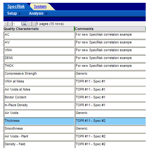
Figure 107. Screenshot. Quality characteristics for selection in SPECRISK.

Pay Equation Setup

The next step is to make sure the necessary pay equations are included as part of the setup procedure. In this case, none of the above pay equations had been previously entered into this particular installation of SPECRISK. However, the pay equation wizard makes it easy to enter these three pay equations as linear compound equations.

Density

Figure 103, the density pay equation, is shown in figure 108 as it appears after entry into the pay equation wizard.

Figure 108. Screenshot. Input of compound linear pay equation for density.

Following the input of the equation coefficients, it can be helpful to plot the resulting pay equation to check for potential errors and discontinuities. This is accomplished by clicking the “Graph” tab in figure 108, which displays the plot shown in figure 109 in which the green and red segments represent the equation segments defined in figure 108.

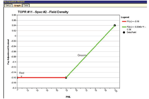
Figure 109. Screenshot. Plot of density pay schedule graph with minimum PA = -0.16.

Air Voids

The pay schedule for air voids is entered in the pay equation wizard in the same manner as shown for density in figure 108 and is graphed in figure 110.

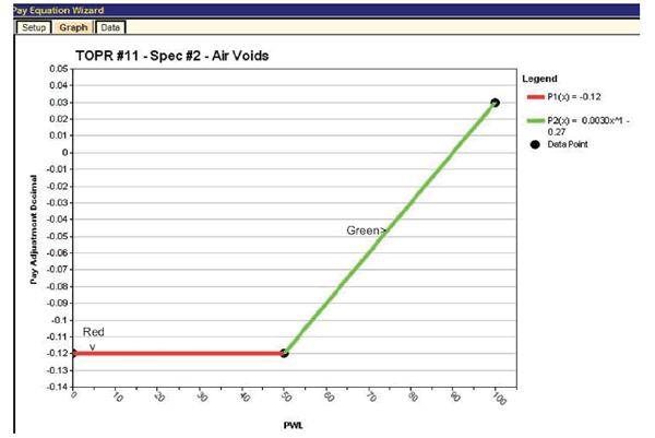
Figure 110. Screenshot. Plot of air voids pay schedule graph with minimum PA = -0.12.

Entering Data into Simulation Profile

Initial setup for simulation profile follows the same steps described in the "Entering Data into Simulation Profile" section for specification 1. In this example, the initial profile with all three quality characteristics can be found with the name "TOPR Number 11 — Specification Number 2 — HMA." The user clicks on it to select it, then right-clicks to select "Insert New Record Like This" in the drop-down window, as shown in figure 111.

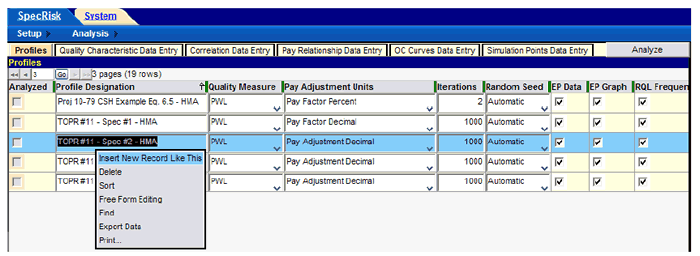
Figure 111. Screenshot. Entering a new simulation profile.

This action causes a new simulation profile line to be added at the end of the list. The new profile is given a name, and a value of 1,000 is entered for the number of iterations.

Next, the information from the profile that has been copied is checked to match the "Acceptance Procedure Synopsis" section. This will consist primarily of removing any reference to the thickness quality characteristic, which has been eliminated from this analysis. To begin, the user selects "Quality Characteristic Data Entry" and deletes thickness by highlighting the appropriate row with a left click and then right-clicking to bring up the dropdown menu shown in figure 111. To delete thickness, the user clicks on "Delete." The user moves successively to the right across the screen to select the remaining yellow buttons and continues to delete all references to thickness.

Figure 112 shows the "Quality Characteristic Data Entry" screen after the thickness characteristic has been deleted.

Figure 112. Screenshot. Modified quality characteristic data entry screen.

Since no information regarding correlation of the quality characteristics was provided for this example, it was assumed for the original run that all correlation values are zero (the default condition for SPECRISK) and no changes are required to the "Correlation Data Entry" tab.

The individual PAs are directly additive for this example. In the "Pay Relationship Data Entry" tab, the appropriate selection of "Sum" in the "Pay Relationship" column had been made initially, and no change is required.

The "OC Curves Data Entry" tab allows the input of user-selected levels of PA for which OC curves will provide the likelihood of achieving this level of adjustment, or higher, at various levels of as-constructed PWL. This result will be accessible by selection of the "Multiple OCs Graph" in the lower section of this screen after the analysis has been run. The previously entered levels of PA will be sufficient for this analysis.

The remaining input tab on the profile screen is "Simulation Points Data Entry." By default, SPECRISK will analyze all possible combinations of quality levels among the selected quality characteristics in PWL increments of 10. This usually provides a fairly complete picture of the performance of the acceptance procedure over the entire range of possible quality-levels, so no additional increment levels need to be added.

Preliminary Analyses

Following the input of essential entries necessary to analyze the specification, it is customary to do a preliminary analysis by entering a few key quality level combinations rather than a performing a complete analysis. After entering a few quality level combinations in the lower table, analysis is initiated by clicking "Analyze Selected" near the lower right corner of the profile screen. The results of one of these runs are shown in figure 113. This analysis can provide almost immediate results at quality levels of interest and may also allow the user to spot obvious input errors.

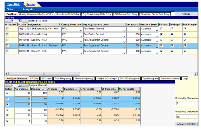
Figure 113. Screenshot. Preliminary run using "Analyze Selected."

One technique that is frequently used when running "Analyze Selected" is to run duplicates of some combinations of quality levels to get an impression of how repeatable (e.g., reliable) the results are. Since the analysis technique used in SPECRISK is computer simulation, it is normal for successive runs (i.e., using automatic random seed numbers) to give slightly different results, and the results will be more variable the smaller the number of iterations that are used. This particular simulation, using two quality characteristics, is considerably less computationally intensive than simulations using four or five characteristics. Thus, it was possible to obtain results very quickly using 1,000 iterations for these trial runs (as indicated in the upper table in figure 113). With 1,000 iterations, it is common for the results to be in good agreement.

One combination of particular interest occurs at the formal AQL when each individual quality characteristic is precisely at its respective AQL. Since both individual pay equations produce a PA of zero, (i.e., 100 percent payment) at PWL = 90, this is the inferred AQL. This level of quality has been duplicated in the lower table in figure 113, as indicated by the two highlighted rows. The first run produced exactly the desired average PA of zero, while the second one was very close. Therefore, this run has provided two important pieces of information—the acceptance procedure properly accepts AQL quality at full payment, and this result appears to be repeatable.

A similar test was run in the fourth and fifth analysis rows of figure 113. In this case, both characteristics have been set at PWL = 50, which would generally be regarded as a poor quality lot. Again, the results are very consistent, both being close to a PA of -0.25. The SHA must judge if the amount of payment withheld is reasonably appropriate for this level of quality.

Another common type of test includes setting the independent variables at their extremes, where it is often possible to deduce what the correct result should be. In the first row in figure 113, both quality characteristics have been set at their maximum possible value of PWL = 100. Figure 103 and figure 106 produce incentive (bonus) PAs of +0.04 and +0.03, respectively, when all characteristics are at PWL = 100. Since these PAs are additive, the net overall PA is +0.07, as correctly reported in the first row of figure 113.

At the other extreme, all quality characteristics have been set at the minimum value of PWL = 0 in the last row in figure 113. Again by inspection, it can be seen that density and air voids receive minimum PAs of -0.16 and -0.12, respectively, at PWL = 0. Therefore, when both quality characteristics are at PWL = 0, the overall PA is calculated as -0.16 + (-0.12) = -0.28, as borne out in the last row in figure 113.

These results are a strong indication that the many inputs have been entered properly, and it is reasonable to conclude that the software is performing the analyses correctly. At this point, it is appropriate to proceed with some additional preliminary analyses of interest.

This specification has virtual RQL provisions in that when PWL < 50, the SHA has option to reevaluate either density and air voids, or both. It is of interest to know what the typical PA will be when the quality levels are poor but not poor enough to trigger these provisions.

To answer this question, the run shown in figure 114 is made. For this test, each characteristic is set at a low quality level of PWL = 50, while the other is set at the maximum quality level of PWL = 100. As in the previous test, the quality level combinations have been duplicated to get a reading on repeatability. All the results appear to be very repeatable, and the PAs when individual characteristics are set at PWL = 50 are approximately -0.07 and -0.11 for air voids and density, respectively. The SHA will have to decide if this provides adequate protection against these low levels of quality, but SPECRISK has provided information upon which these decisions can be made.

Figure 114. Screenshot. Comparison of individual low levels of quality.

An additional series of tests will be useful to provide a reasonableness check of the preliminary results. For these tests, each individual quality characteristic is varied throughout the complete range of possible quality levels, while the other is held at the AQL of PWL = 90. These results are presented in figure 115 and figure 116.

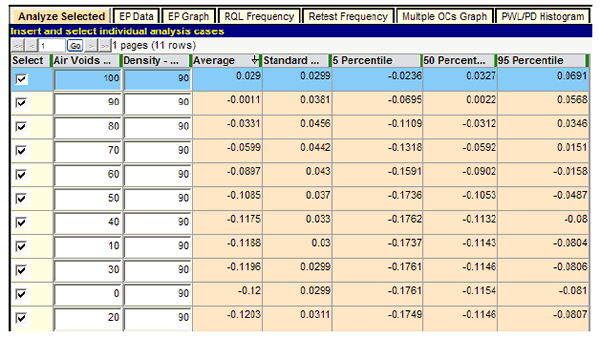
Figure 115. Screenshot. Extended test of air voids PAs.

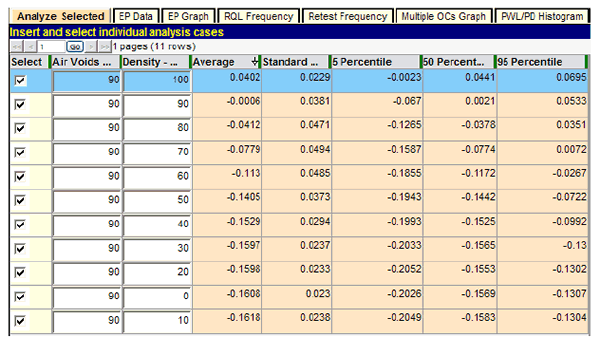
Figure 116. Screenshot. Extended test of density PAs.

Several interesting observations can be made from this last group of test runs. As each quality characteristic is decremented by PWL = 10 while the other characteristic is held constant at the AQL of PWL = 90, the expected PA (average) decreases steadily until its individual minimum PA is approached. Beyond that, any decrease is very small and is due partly to the small variability of the sum of the other adjustment (which randomly varies about zero, the expected value at the AQL). As a result, it is possible on any particular run for the lot PA to reach a minimum just slightly below the minimum PA for the characteristic under test, and the last two or three rows can go out of order due to random chance, as seen in figure 115 and figure 116.

These two figures also show that at the point at which both characteristics are at the AQL level of PWL = 90, the resultant expectant PA (average) is almost exactly zero (full payment). This reinforces the conclusion that this is an unbiased pay schedule that will award 100 percent payment in the long run at the AQL.

Ambiguity at the AQL

Before proceeding with the complete analysis, there is an additional topic that warrants discussion. As noted previously, the condition at which all quality characteristics are simultaneously at their respective AQL values can be regarded as a formal definition of an AQL lot, when full payment should be awarded. But when analyzing multicharacteristic acceptance procedures, it is apparent that there are many other combinations of quality levels that will also produce full payment. Furthermore, when an attempt is made to develop performance models of expected pavement life as a function of as-constructed quality, it is discovered that this may be a very appropriate feature of multicharacteristic acceptance procedures. In other words, it is not uncommon to expect a slight surplus of quality in one quality characteristic to offset a slight deficiency in another quality characteristic (within reasonable limits).

To study the performance of the specification at hand in terms of this offsetting property, a series of tests can be run for which each quality characteristic in turn is cycled from its AQL downward as the other characteristic is held at the maximum quality level of PWL = 100. In this manner, it is possible to discover just how low in quality each characteristic can go with the lot as a whole still receiving full pavement. The first such test is for air voids, as shown in figure 117.

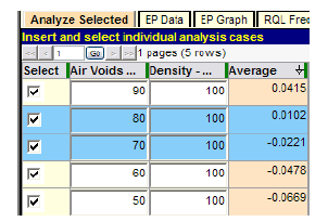
Figure 117. Screenshot. Determination of critical level of air voids quality.

In figure 117, the air voids characteristic is tested over a sufficient range of PWL (90 to 50) to observe that somewhere between PWL = 80 and 70, it will produce an expected PA of zero (100 percent payment) and thus be equivalent to an AQL combination. A second run is shown in figure 118 to determine this critical value more precisely.

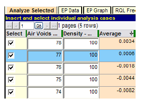
Figure 118. Screenshot. Precise determination of critical level of air voids quality.

Figure 118 shows that full payment (PA = 0) occurs at a point very close to an air voids quality level of PWL = 77. The SHA must decide whether or not full payment is acceptable for this combined level of lot quality in the two characteristics. The same series of tests was run for density, and the final result is shown in figure 119.

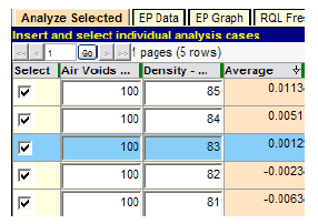
Figure 119. Screenshot. Determination of critical level of density quality.

Figure 119 indicates that full payment (essentially PA = 0) can occur when density quality is as low as PWL = 83. Provided the SHA is satisfied with this possibility, this may be regarded as a suitable acceptance procedure, especially if it has had a history of encouraging good quality on the part of the construction industry.

Time-Saving Procedure

SPECRISK is capable of performing a full factorial experiment by simulating all combinations of quality levels in all of up to five quality characteristics, typically in PWL increments of 10 (or PD = 10) and graphing most of these results as selected by the user. With a relatively large number of simulation replications, a complete analysis such as this may require several hours of computational time, depending on the speed of the computer on which it is run. However, it is often possible to obtain certain key results without such a time-consuming effort.

A useful series of quality levels for analysis consists of all possible combinations of AQL and RQL values for all quality characteristics. This subset of data can be selected upon completion of the complete analysis, but it is also relatively easy to set up for fast results with "Analyze Selected."

For the full complement of five quality characteristics, this would require entry of 2⁵ = 32 rows of quality combinations. For the specification currently under analysis, there are only two quality characteristics, which require only 2² = 4 lines of data. The AQL has been implied as PWL = 90 for all quality characteristics because that equates to a PA of 0. For air voids and density, the RQL has been taken to be PWL = 50 because that is the level of quality below which the agency could decide to reject the work. The experimental design and the results of this analysis are shown in figure 120, where the results for the AQL/RQL combinations are presented.

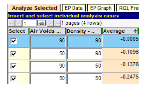
Figure 120. Screenshot. Test with all AQL/RQL combinations.

Figure 120 shows that when both quality characteristics are at the AQL of PWL = 90, the resulting average PA is essentially zero, representing full payment for quality precisely at the level specified. The remaining three lines represent successively poorer combinations of quality and demonstrate that the associated expected pay levels decline accordingly.

In order to address the positive side of the pay schedules, figure 121 shows the level of incentive PA the quality-conscious contractor can receive by controlling production at or near the maximum quality level of PWL = 100. Although in theory no lot can achieve complete perfection as indicated by a PWL level of 100 percent, it is possible for good quality lots to test out at PWL = 100 because of random sampling variability, and they often do. Whenever this occurs, the result in figure 121 indicates the contractor will receive an expected (average) PA = 0.07, which is a positive incentive (bonus) payment of 7 percent.

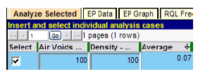
Figure 121. Screenshot. Demonstration of positive incentive provision.

Full Analysis

For many agencies, the preliminary analyses may be sufficient to confirm that the acceptance procedure is working satisfactorily or demonstrate that modifications need to be made. For those desiring more detailed information, a full analysis can be run. One major advantage of a full analysis is that it provides access to the many graphical and tabular displays of data that SPECRISK can provide.

The most important graph for SHAs and contractors is the EP graph, which illustrates how payment is related to quality delivered. The EP graph produced by the full analysis is shown in figure 122.

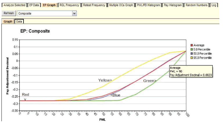
Figure 122. Graph. EP graph available with full analysis.

The red line in figure 122 represents the average (or expected) PA, and the figure represents the composite, or overall, combined PA resulting from the PAs for the individual quality characteristics. The red line shows the gradual increase from the minimum PA of -0.28 at PWL = 0 up to the maximum PA of 0.07 at PWL = 100. This graph allows both the SHA and its contractors to see exactly how the acceptance procedure will perform and what the consequences of both good and poor quality control are likely to be.

For example, highway specification engineers can see that this specification awards 100 percent payment at the AQL of PWL = 90. Figure 122 also illustrates the hover feature of SPECRISK. A quantitative reading can be obtained from the graph by hovering the cursor close to the point of interest. In this case, a PA of 0.0023 (essentially zero) is expected at the AQL of PWL = 90.

With this information, SHAs can judge if the acceptance procedure is both effective and fair, and contractors can see the benefits of targeting quality levels at or above the AQL. The highway agency has an abiding interest in confirming that the rate at which payment declines as the quality drops below the design quality level is both effective and appropriate. This graph also communicates to the contractor the seriousness of the specifications and that poor quality likely will be detected and assessed appropriate pay reductions. However, this also illustrates the potential monetary benefits available to the contractor who exercises good quality control and produces work at or above the AQL.

Figure 123 shows how the "Multiple OCs Graph" can provide still more information on this subject. Like figure 122, the user has again selected the composite analysis. The legend at the right of the figure lists several PA levels previously entered by the user, and the blue line represents full payment (PA = 0).

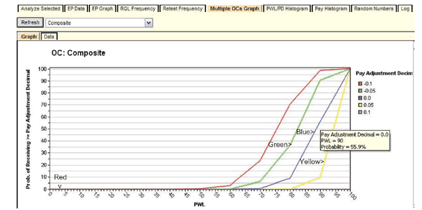
Figure 123. Screenshot. Display of multiple OCs graph.

In figure 123, the hover feature shows the probability of achieving full payment (or greater) when the work is controlled precisely at the AQL of PWL = 90 to be 55.9 percent (0.559), meaning that there will be slightly more positive PAs than negative PAs. In this case, the contractor who can successfully produce at the AQL can expect to average somewhat better than full payment in the long run because the positive PAs will outweigh the negative PAs to some extent (consistent with the result in figure 122).

This graph can also provide guidance for the contractor who might prefer to control production so that there will more “bonuses” than reductions throughout the course of a project. For example, if a contractor wished to obtain bonuses about 80 percent of the time, a production level of quality of about PWL = 95 would be required. If it were relatively easy for a contractor to achieve this level of quality, this might well be a profitable strategic decision. In any case, SPECRISK has provided information to help in making this decision.

Analysis Summary and Conclusions

Significant findings unique to the analysis in this appendix were as follows (additional conclusions for the full scope of this specification are listed in the main body of the report):

• One of the important features of these analyses is to confirm that the pay schedule is capable of paying 100 percent as a long-term average (i.e., PA = 0) when the quality of production is at the level that is defined as acceptable in the specification. In this example, the tests confirmed that the overall combined PA was essentially zero.
  
  
• The formal definition of an AQL for a multicharacteristic acceptance procedure should be that combination of quality levels for which each quality characteristic is precisely at its respective AQL value. There are essentially an unlimited number of equivalent AQL combinations for which the resultant composite PF will turn out to be PA = 0. The important thing to check is whether one or more such combinations might exist for which the agency would consider it clearly inappropriate for full payment. Example test runs were presented in figure 117 through figure 119. The SHA using the specification is required to make the final decision.
  
  
• The "Acceptance Procedure Synopsis" section for this specification indicates that for both density and air voids, the resulting PAs (in decimal form) are applied to a flat rate of $40 per ton. In the original analysis that included thickness, the dollar value of the PA was obtained by multiplying the decimal adjustment by $1.90 by the area (square yards) by the thickness (inches), which works out to be very close to $40 per ton. It is presumed that the specification designers took this approach as a countermeasure to possible temptation on the part of contractors to unbalance their bids for strategic advantage. As such, it should be an effective deterrent.
  
  
• Figure 115 and figure 116 included duplicate runs to demonstrate how repeatable the independent simulation results would be with 1,000 iterations. For preliminary exploratory work, the goal is to strike a reasonable balance between precision of results and speed of response. The checks shown in these two figures illustrate that 1,000 iterations will usually be satisfactory. In general, it is desirable to work at the highest practical level of precision, and it is usually desirable to use an even greater number of iterations for final results.
  
  
• Figure 122 and figure 123 show graphs describing payment results to be expected with this acceptance procedure. This information will be of particular interest to both the SHA and the construction industry.