U.S. Department of Transportation
Federal Highway Administration
1200 New Jersey Avenue, SE
Washington, DC 20590
202-366-4000
Federal Highway Administration Research and Technology
Coordinating, Developing, and Delivering Highway Transportation Innovations
| REPORT |
| This report is an archived publication and may contain dated technical, contact, and link information |
|
| Publication Number: FHWA-RD-01-113 Date: October 2002 |
Publication Number: FHWA-RD-01-113 Date: October 2002 |
The back-calculation procedure and steps reported in this document were used to determine the layered elastic properties (Young's modulus and the coefficient and exponent of the nonlinear constitutive equation) from deflection basin measurements for all LTPP test sections with a level E data status. The report summarized the reasons why MODCOMP4 was selected for the computations and analyses of the deflection data, provided a summary of the results using the linear elastic module (Young's modulus) for selected test sections, and identified those factors that can have a significant effect on the results. Some of the highlights and findings from this study and recommendations for future activities in support of accomplishing the overall LTPP objectives are included in this section of the report.
One of the reasons that MODCOMP4 was selected as the back-calculation program was that it has the capability to consider different nonlinear constitutive equations. It was initially hypothesized that the use of nonlinear constitutive response equations would significantly improve on the number of solutions with low RMS errors (less than 2 percent). However, significantly less than 50 percent of the test points were found to have solutions, with the RMS error less than even 4 percent using different nonlinear constitutive equations. Thus, the hypothesis was found to be untrue or incorrect using the existing software and deflection data measured at the LTPP sites.
Back-calculation of elastic properties, however, is not an exact procedure or science and requires manual interaction with the user, especially when using the nonlinear module of MODCOMP4. More importantly, more sensors are probably needed to define clearly the deflection basins for back-calculating the nonlinear elastic properties for the pavement layers and subgrade soils, especially for pavement structure with more than two layers. Thus, the back-calculation of nonlinear elastic layer properties should not be completed on a mass-production basis.
Results from this study do provide elastic layer properties that are consistent with previous experience and laboratory material studies related to the effect of temperature, stress state, and season on material load-response behavior. The following lists some of the important observations or findings from this back-calculation study.
The results from this study have shown that elastic layer properties, especially Young's modulus, can be computed from deflection basins and provide the pavement engineer with useful information on the pavement's structure and subgrade condition. It is recommended that a detailed analysis of these results be completed to demonstrate their usefulness and to identify problem or unique test sections. It is also recommended that deflection basins, measured in the future along the LTPP test sections (especially the SPS test sections), be used to compute the elastic properties of the pavement and subgrade layers in order to evaluate changes in the layer moduli with time or age. Completing the back-calculation process of the nonlinear elastic properties on a production basis, however, is not recommended.
Von Quintus and Killingsworth previously recommended a set of C-values for adjusting the back-calculated moduli from FWD deflections to laboratory-measured resilient moduli or vice versa.(1) These C-values were determined from back-calculated layer moduli using the MODULUS and WESDEPTH software packages. In all probability, these C-values are dependent on the back-calculation software package used. Thus, the back-calculated Young's modulus derived from MODCOMP should be compared with laboratory-measured resilient moduli for the different pavement materials and subgrade soils.
The use of MODCOMP, MODULUS, and other software packages to calculate elastic layer properties from FWD deflection basins does not provide reasonable solutions in every case because these programs are not perfect simulations of real-world conditions. Each program has limitations and inaccuracies in simulating the deflection basins. However, as quoted from Von Quintus, Bush, and Baladi in the 1994 International Conference on NDT and Back-Calculation of Moduli:(13)
In summary, most participants concurred that there needs to be a standard baseline of values from which to compare a project, material, or pavement base and that one should not become paralyzed by the imperfection of the procedures. More importantly, research must be merged into practice on a consistent basis and one way to accomplish this is through the standardization process. As such, a procedure needs to be standardized and that procedure should concentrate on user oriented issues.This study has attempted to implement and apply existing standardized procedures (ASTMD5858 and FHWA-RD-97-076) to back-calculate Young's modulus and the nonlinear elastic properties for each pavement and subgrade layer. Results from this extensive effort, as well as from other studies, such as FHWA-RD-97-086, are promising and have shown that reasonable solutions for Young's modulus can be obtained. These computed parameters have been included in the LTPP database for future pavement performance and material studies. These results also provide a baseline of solutions and elastic properties for which the results from future studies can be compared and improved upon.
Another quote from Von Quintus, Bush, and Baladi at the 1994 International Conference reads as follows:(13)
The question, however, is still: what is the reliability of these values? Specifically, it was the general consensus of the panel and attendees that the accuracy of back-calculated moduli is model dependent and unknown, as well as those values measured in the laboratory because there is a diversity of opinion on the simulation of field conditions in the laboratory. For example, there is controversy within the industry on whether back-calculation procedures should be based on a dynamic or static analysis, and what values actually represent the truth, both in the laboratory or from field measurements.Unfortunately, the relationship between the computed parameters from this study and resilient moduli from the laboratory repeated-load testing has not yet been established.
Introduction
Back-calculation is a process for estimating the elastic layer modulus in pavement structures that represent in situ conditions under a test load. Back-calculation gets its name from the fact that a load of known size and shape is applied to the pavement and deflections are measured by sensors at known distances from the load. Theoretical predictions are made of the deflections, assuming certain layer properties, and those properties (usually elastic layer modulus) are adjusted until the calculated deflections match the measured deflections within a reasonable RMS error (goodness-of-fit between the measured and calculated deflection basins).
Back-calculation of elastic properties is usually performed with static-linear analyses, and there are numerous computer programs or software packages that can be used to calculate the elastic properties of each layer. The MODCOMP4 software package was selected and used for analyzing the LTPP deflection data, because (among other features) it is capable of doing back-calculation for massive quantities of deflection data using both linear (Young's modulus) and nonlinear (stress dependent elastic modulus) approaches for materials characterization.
Nonlinear materials are those for which the modulus depends on the applied stress (i.e., stress-dependent) and is not a single number but a relationship between modulus and stress. Numerous mathematical forms have been used to represent the relationship between modulus and stress. The particular relationship adopted for a layer material is referred to later in this document as a constitutive equation.
Purpose of User's Guide
The back-calculation procedure explained in this appendix is a tool that agencies can use in the future to update the computed parameters (elastic properties) of each layer for the LTPP test sections as more and more deflection basin data are measured over time. This User's Guide is intended to accomplish the following objectives:
The back-calculation process is a series of DOS-based programs, and the user must be familiar with the use of these types of programs to complete the process. The user should also be experienced and knowledgeable in the back-calculation process and familiar with the LTPP database. The audience intended for this User's Guide includes pavement materials and design engineers; research engineers; pavement management engineers; and other professionals in Federal, State, and local government; academia; and in private industry.
Back-Calculation Procedure Overview
The overall operational process for back-calculating the layer modulus basically follows the procedure outlined by Von Quintus and Killingsworth in publication number FHWA-RD-97-076(1) and the Instructional Guide for Back-Calculation and the Use of MODCOMP.(10) This process was developed for back-calculating massive quantities of deflection data that are stored within the LTPP database (the IMS or a centralized location).
The procedure used to back-calculate the elastic properties of each layer for the LTPP test sections consists of a number of operations. This User's Guide identifies and discusses all of the operations (programs and decision functions) included in this process. The procedure is not fully automated but is an iterative process between the different programs and requires engineering judgment of the user. The following lists those major steps that are used in the process:
Step 1 -- Extract Data from IMS
Step 2 -- Preprocess the Extracted FWD Deflection Basin Data and Section Classification
Step 3 -- Create Input Files for MODCOMP4
Step 4 -- Trial Computations and Modification of Inputs
Step 5 -- Back-Calculate Young's Modulus and the Nonlinear Elastic Properties Using MODCOMP4
Step 6 -- Extract Elastic Properties and Create Summary Output Files
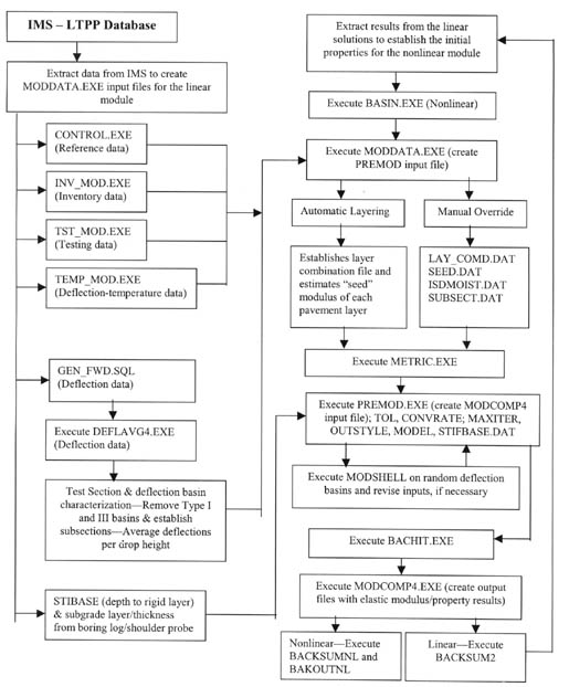
An important fact regarding future use of the procedure is that the LTPP database is dynamic, and the programs that are used to extract the data were written based on the database that existed in 1998. These programs may need to be revised as the LTPP database is updated and changed over time. The following identifies and describes briefly the programs used to accomplish the above operations. Figure 31 is a flow chart of the back-calculation procedure.
At the conclusion of this process, the detailed results for each back-calculation are available in the stored MODCOMP4 summary and output files, and the specific results (layer modulus for each layer and load level for the linear solutions, and the modulus for the highest load level and the coefficients and exponents for the selected equation form for each layer for the nonlinear solutions) are stored in separate files. These files also include for each solution the section identification, location within the section, date and time of deflections, pavement layer temperatures, layer thickness and material type, and, for nonlinear solutions, the model that was used for each layer. The files are then manipulated to produce tables suitable for loading into the LTPP Oracle® database.
Step 1: IMS Data Extraction
The user must first designate or identify what test sections are to be back-calculated. The Technical Services Support Contractor (TSSC) will normally execute the data extraction programs or packages to retrieve the required data and other information. These programs and their use are defined below.
Programs INV_MOD, TST_MOD, TST_MOD2, and TEMP_MOD acquire data for all sections from the relevant tables in the LTPP database. The resulting files can be considered "archival" in the sense that they are obtained once and used without modification during a particular series of back-calculation.
Note 1: As more testing data and more deflection basins are acquired and added to the IMS, they should be regenerated at the beginning of each back-calculation exercise.Note 2: The LTPP database is dynamic, and the programs that are used to extract the data from the IMS were written based on the database that existed in 1998. These extraction programs may need to be revised as the LTPP database is updated and changed over time.
Note 3: The inventory data are used only as a backup when other data are missing or unavailable in the database, with the exception of asphalt viscosity data. Viscosity data are included only in the inventory data tables in the LTPP database.
All of these extraction programs are executed with the following syntax:
where <connect string> is the character string <username/password@database>. Obviously, these programs must be executed by an agency that has a connection to the LTPP database -- normally, the TSSC.
Program CONTROL is similar but not identical in usage. The syntax for it is:
where <low state> and <high state> are the LTPP State or Province codes for the first and last State to be included in the run. One may, therefore, generate control files for one State at a time, a group of States, or all the states at once (where "State" refers to both States and Provinces). One may generate output for all the States and later break the resulting file down into smaller groups of test sections in an editor (a useful procedure if one is dependent on TSSC for running the program).
For convenience, this input guide refers to the output files of the above programs as INV_MOD.lis, TST_MOD.lis, TST_MOD2.lis, TEMP_MOD.lis, and CONTROL.lis. In the first three, remembering that TST_MOD2.lis is the same as TST_MOD.lis except that it provides data where available for construction number 2 (rehabilitation events), the same set of information is provided for all layers; all layers will have blank fields where the field is inappropriate for the material type of that layer. These programs convert metric density to English units but otherwise leave the values in the units used in the LTPP database. The LTPP database was undergoing a metrication process, so the user must be careful about using the programs. Program MODDATA, which uses the output of these programs, was written to use English units throughout.
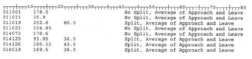
TEMP_MOD.lis provides both the hole depths and the temperature readings at those holes (which are drilled such that top, middle, and bottom temperatures are obtained) during the deflection testing for each section visit, as well as the date, time, and location of the hole. No conversions are done to the temperatures, so they are output in the units present in the LTPP database (metric after May 2000).
Sample data:
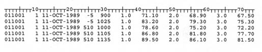
For section 011001 on October 11, 1989, at stations -5 and 510, we have holes in the pavement of 1.0, 2.0, and 3.0 inches deep, with the indicated temperatures (F) at times from 0900 to 1135.
The last type of data obtained from the IMS is the data for the deflection basins. An SQL script, GEN_FWD.SQL, (which may be edited to obtain data for GPS, for SPS, or for seasonal sites), is run that produces a second (very large) SQL script that obtains the deflections in English units of mils (.001 inch), peak loads (in ksi), and air and pavement temperatures (in degrees F) for each section and visit date, and writes the data for each section (all visits) to a separate file. Again, this requires a connection to the IMS and would most probably be done by the TSSC. The output files from this process are labeled F<state_code><shrp_id><construction_no>.lis.
Step 2: Preprocess the FWD Deflection Data -- Execute DEFLAVG4
As discussed above, the deflection data acquired are passed through program DEFLAVG4, which performs several operations on the data. Deflection data from the IMS consist (normally) of basins from 12 drops (rigid pavements) or 16 drops (flexible pavements), 4 at each drop height, or nominal load. The deflections for each drop at a given drop height are normalized by the load for that drop; the normalized drops are then averaged and the results multiplied by the average load for that drop height. This is done for each of the seven sensors.
The program is run by typing in the command prompt: DEFLAVG4<space><Data File Name><return>. The use of the DOS FOR-DO loop will make it possible to execute DEFLAVE4 on all FWD data files in a subdirectory with one command.
In performing these operations, the deflection basins are checked for nondecreasing deflections with increasing distance from the load; if this occurs, the drop is omitted from the average. In addition, a test for variation based on that used in the FWD software itself is applied: If an individual (renormalized) deflection value differs from the average by more than (0.08 + 1 percent [average deflection]) mils, that difference is calculated for all sensors and summed. The drop having the largest sum is excluded, and the average is recalculated. If necessary, this process is repeated, leaving only two drops. If they differ from their average by more than the above amount, the average is accepted but marked as "variant" in the output file. The criteria of 0.08 mils and 1 percent are from the stated accuracy specifications on the FWD unit itself.
If all the drops at a given location and load have nondecreasing deflections, they are all discarded. If all but one is discarded, the remaining value is used, but obviously there can be no check for variation in this case. The number of drops contributing to the final average is recorded in the output file for each drop height; where only two remain and one or more sensors show variation, the deflection values for those sensors are so indicated in the output file.
The program name DEFLAVG4.exe indicates the version used for flexible data with four-digit years in the dates. (DEFLAV_R.exe is the same except that it is used with rigid pavement deflection basin data, and uses only data from mid-slab basins [lane numbers J1 or C1].) Output files have the same file name as the input file, with an extension ".AVG." A "log" file is written for each run, showing the details of the averaging and drop exclusion process. This file has the ".LOG" extension.
Note 4: Program BASIN is executed external to the back-calculation process to determine the load-response (figures 2-4) and basin (figures 5-8) classification of the deflection basin data. Figure 32 illustrates the flow diagram for characterizing the deflection basin measurements. The load-response classification assists the user in selecting the initial constitutive equation for the nonlinear module of MODCOMP. The BASIN program is not needed for the linear module.
Example data file for one station, two load heights (F0110011.lis):
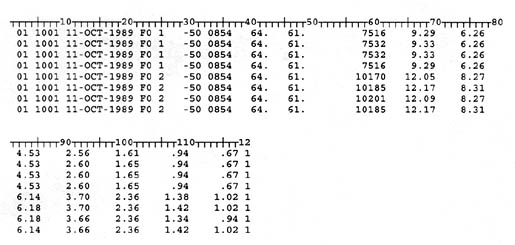
The section (State code and SHRP_ID), date, lane, load height, station, drop time, air temperature, and pavement temperature are present for each drop, followed by the load, the seven deflections, and the construction number.
Example output file for the above input data (F0110011.avg):
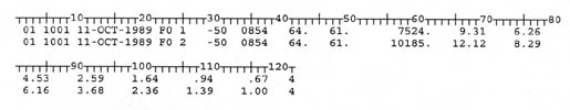
The single digit at the end of the output line is the number of drops that contributed to the average; the construction number is retained as the last digit in the file name.
Step 3: Create Input Files for MODCOMP4
Execute MODDATA
MODDATA reads information from the files discussed above and creates an output file consisting of identification, layer information, and deflections for each location at which deflection basins were obtained (and which passed through the DEFLAVG programs). Most importantly, it derives initial estimates for modulus and Poisson's ratio for each layer from the material types and physical properties of those layers. Initial estimates for the layer modulus are computed in accordance with a regression equation or obtained from a tabular listing of values for different materials, whereas estimates of Poisson's ratio are automatically obtained from a tabular listing of values for different materials (refer to table 4).(1,15)
Automatic Layering Definition
For sections having more than five layers, MODDATA performs layer combinations according to rules established by LTPP in 1993, unless the user overrides the process with desired specific layer combinations.(15)
Note 5: Although the original back-calculation program used with MODDATA could handle only five layers total (including rigid base) and MODCOMP4 can handle many more, it is considered inappropriate to solve for more than five layers when using MODCOMP4.
To run MODDATA, it is best to establish some standard file locations, or paths, ahead of time. The following are suggested:
<exepath> The location of the executable programs in this process.
<commpath> The location of common data files used for multiple runs of MODDATA on different deflection data (e.g., the IMS extraction data files).
<deflpath> The location of deflection data files generated by DEFLAVG4 or DEFLAV_R.
<sectpath> The location of files unique to a specific run of MODDATA.
MODDATA can use (but does not require) several input files in addition to those containing the IMS extraction data; when executed, the program requests that each file name be entered in response to a labeled prompt, shown as follows, with the recommended location for each:
Enter name of REFERENCE file <sectpath>F0110011.CNT
Enter name of INVENTORY DATA file <commpath>INV_MOD.LIS
Enter name of MATERIALS TEST file <commpath>TST_MOD.LIS
Enter name of DEFLECTION TEMPS file <commpath>TEMP_GPS.LIS
Enter name of DEFLECTION DATA file <deflpath>F0110011.LIS
"NONE" CAN BE ENTERED FOR THE NEXT FOUR FILENAMES
Enter name of IN-SITU DENSITY DATA file <commpath>ISDMOIST.DAT
Enter name of EXTERNAL LAYER COMBINATION file <commpath>LAY_COMB.DAT
Enter name of EXT. LAYER MODULUS INPUT file <commpath>SEED.DAT
Enter name of STATION SPLIT-LOCATION file <commpath>SUBSECT.DAT
Enter name of ERROR OUTPUT file <sectpath>F0110011.ERR
Enter name of SUMMARY OUTPUT file <sectpath>F0110011.OUT
Enter name of DATA OUTPUT file <sectpath>F0110011.DAT
Each file shown in <commpath> will normally contain data for many test sections, and in the case of TEMP_GPS, numerous dates per test section. F0110011.CNT, the control file in the example shown, will have multiple dates for the test section 011001, construction number 1. The program will search each file for the test section identification 011001 and will search for the specific dates in TEMP_GPS and in F0110011.LIS. If a control file containing section identifications for multiple sections is used, the data for each section will be sought within each file.
Manual Override or Optional Inputs for MODDATA. The optional input data files ISDMOIST.DAT, LAY_COMB.DAT, SEED.DAT, and SUBSECT.DAT provide additional data and allow the user to override the program choices.
Note 6: Format details are provided later for these files.
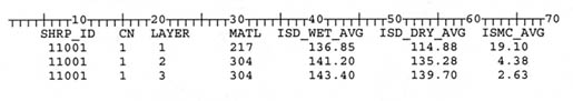
ISDMOIST.DAT provides in situ densities (from nuclear density gauge measurements) and moisture contents for base and subgrade layers where such measures are available. The values in the IMS were obtained at specified depths from the surface; those depths must be converted to layer numbers before they are useful in this application, and that is most easily done by hand-external to the program. Averages are taken of multiple data values for a single layer where such exist. These values are needed for nonlinear back-calculation where the weight of the material overlaying a given layer is taken into consideration in calculating the stresses within that layer.
LAY_COMB.DAT allows the user to control the process of layer combination externally, based on previous back-calculation attempts or on study of the standard layer combination performed by MODDATA. If any combination is specified in LAY_COMB, all desired combinations must be specified and the automatic process is turned off.
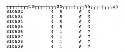
In this example, the first four sections of the Alberta SPS5 project are handled differently from the last four: In the first four layers, 4 and 5 are combined, and layer 6 is prevented from combining with another layer. In the last four, layer 4 is prevented from combining, and layers 6 and 7 are combined.
SEED.DAT allows the user to bypass the internal calculation or lookup of modulus estimates for specific layers and to specify the value to be used. The values entered apply to the original layering, not the final layering after combination. Therefore, to ensure that a layer after combination has a specific value, all components of that combined layer must be given that value. An example follows:
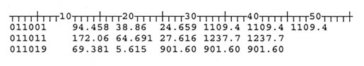
In each of the three sections shown, the asphalt top layers were combined in the final output.
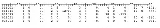
SUBSECT.DAT allows the entry of a station value that serves to split the section into two subsections; thickness of each layer from the approach testing area will be applied to all deflection stations less than that value, and those from the leave testing area will be applied to the remainder of the stations. Special values for this station exist: +9999 will enable the use of average layer thickness for all stations (the default situation), and -9999 will cause thickness values from the "nearest end" to be used for analysis of deflections taken in the testing areas and the average values for deflections obtained within the section.
Note 7: The "average values" referred to here are the values from LTPP database table TST_L05B, which are values considered "representative" of the section; these are often but not always averages of the values from the two ends.
An example follows:
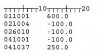
For the first section, the layer thickness from the approach end will be applied to all stations; for the next three sections, those from the leave end will be used. For 041037, those before station 250 will use the approach-end thickness, and those equal to or after 250 will use layer thickness from the leave end.
Program Output.
The output files F0110011.{ERR,OUT,DAT} are to some degree redundant but have specific purposes. The .ERR file contains, in addition to error and informative messages, details of temperature interpolation and of asphalt stiffness calculations. It is not intended to be printed because of its size (it is too large).
The .OUT file contains the original layering, the layering after combining asphalt layers, and the final layering after combining other adjacent layers of similar materials. In this way, the user can see exactly what is being done and make decisions as to whether the automatic process produces a result consistent with the user needs. The .DAT file is the output file used in following the steps in the back-calculation process; it contains the final layer system (with estimated modulus, thickness, Poisson's ratios, material densities and moisture contents, and for pavement layers the interpolated mid-layer temperature) and the average load and deflections at a specific date, time, station, and load height.
Because there are so many input and output files for MODDATA, it is recommended that a "file of file names," or metafile, be established prior to running the program. This can easily be done in a text editor and allows easy corrections of typing errors without starting over from the beginning, as would be required if an error occurred in a file name entry directly into MODDATA. In addition, such a metafile can be stored with the run-specific input (CONTROL) and output files in a compressed (ZIP) file for future reference and/or use. The standard DOS redirection of input from the console to the specified metafile is accomplished using the less-than symbol, as shown below:
MODDATA < metafilename
Execute METRIC
Program METRIC uses the .DAT file output by MODDATA as input and writes out a file, normally with the same file name and an extension of .MET, containing the same information in metric (SI) units for use in MODCOMP4, as follows:
| Item | MODDATA | METRIC | Conversion Factor |
|---|---|---|---|
| Layer thickness | in | m | (= inches*.0254) |
| Layer modulus | ksi | MPa | (= ksi*6.894757) |
| Layer density | pcf | kg/m3 | (= pcf*16.01846) |
| Temperature hole depths | in | micron | (= inches*25.4) |
| Interpolated temperatures | °F | °C | (= [deg F-32]*.555555) |
| Depth to refusal | ft | m | (= feet*.3048) |
| FWD load | lb force | kN | (= lbs*.004448222) |
| FWD deflections | mils | mm | (= mils*25.4) |
Note 8: Deflection location values (in feet) were not changed because they are descriptive only.
Sample input and output files:
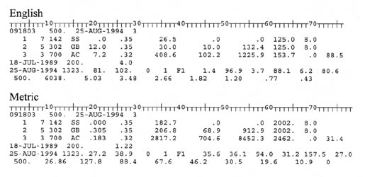
For this example, MODDATA output (English and Metric) for section 091803 (in CT) has three layers after combinations.
Execute PREMOD3
Program PREMOD3 takes data from MODDATA (after passing through METRIC), consisting of multiple average deflection basins for different loads at multiple points on multiple dates, and writes out input data files acceptable to MODCOMP4. For linear back-calculation, one data file is required for each average basin studied; for nonlinear studies, the basins for all loads done at one location and time are included in one data file. A very large number (up to 5,000) of data files can be generated by one run of PREMOD3 (e.g., linear studies for a seasonal site).
The program allows external user control (again, by auxiliary data files) of the choice of sensors associated in MODCOMP4 with a specific layer (usually done after the first run through MODCOMP4 with automatic assignment), the choice of nonlinear models for specific layers, and the choice and depth of a second subgrade layer and/or a rigid foundation.
Note 9: A second subgrade is often used to model the changes of confining and deviator stresses with depth. A rigid foundation can model the actual presence of a very stiff layer at depth or the effect on the subgrade of a nearly vanishing deviator stress and increasing confining pressure at depth, which may make the subgrade material act as though it were a very stiff layer. In addition, for a thin layer or a layer for which the stiffness is considered known, the modulus can be entered as a "known" value, not subject to change by the program.
A metafile can be established for PREMOD3 runs in a manner similar to that for MODDATA, enabling better batch (unattended) operation, if needed, and providing the opportunity for correcting typing errors without restarting the program. This metafile can use the extension .PMD and a file name showing the SHRP_ID, if desired. It will contain responses to questions asked by PREMOD3, as well as the file names (or "NONE") of the files described above. When executed, PREMOD3 asks the user for the following information:
English (E) or Metric (M)
ENTER NAME OF MODDATA OUTPUT FILE: <shrp_id>.MET
ENTER NAME OF STIFF-BASE-DEPTH FILE, or type NONE: STIFBASE.DAT
ENTER NAME OF NON_LINEAR MODELS FILE, or type NONE: MODELS.DAT
ENTER NAME OF SENSOR/FIXED-STIFF FILE, or type NONE: SENSOR.DAT
ENTER LOG FILE NAME FOR THIS RUN: <shrp_id>.LOG
ENTER OUTSTYLE, TOL, CONVRATE, MAX ITER, MODEL NUMBER
(use single quotes on CHAR. inputs)
Because for this project MODCOMP4 was to be run in metric units, the first question is always answered with an M, and the .MET data file output by METRIC is used for the second. Standard names were established for the next three files, as shown above; the log file name is arbitrary, but the above choice is consistent and recommended.
OUTSTYLE is a character variable in MODCOMP4 describing the volume of output requested: BRIE (brief), LONG, or ALL. BRIEF echoes the input and gives final layer modulus. LONG reports the layer modulus for each iteration, and ALL reports intermediate calculations as well; ALL gives very lengthy output and should be used with care.TOL is a single character variable in MODCOMP4 describing the allowable tolerance on the fit to the deflections: values of L (low), M (medium) and H (high) are allowed, H (high) is recommended. This applies only to those sensors assigned to specific layers. H (high) tolerance implies a good fit, not large residuals.
CONVRATE is a numeric value indicating a lower limit on the rate of change of modulus between iterations; 1.5 percent is usually used.
MAX ITER is the maximum number of iterations allowed before the program "gives up"-- usually 15. If this number is reached, either new starting values or new sensor assignments are probably needed.
MODEL NUMBER has the following allowable values and meanings:
0 - Use linear for all layers
>0 - Nonlinear model to be used for -ALL- base/subgrade layers
-1 - Use the bulk stress model (model 1) for base/subbase and the deviator stress model (model 2) for subgrade soil
-2 - Model number to be read in for each layer from external file
With this information, PREMOD3 can generate a MODCOMP4 input data file for each basin (linear) or each set of basins at different load levels but the same location and time (nonlinear).
The auxiliary input files for PREMOD3 allow the user to modify the default behavior of the program and/or of MODCOMP4, as follows:
STIFBASE.DAT provides information on the desired value of depth to stiff base, if the value calculated within PREMOD3 is inappropriate, and the thickness of a top subgrade layer, if such a layer is desired.
Note 10: The internal calculation of the depth to an apparent rigid layer is based on the Texas A&M procedure by G. Rohde, which was taken from the MODULUS 4.0 program.(16)
Values required are the six-character section ID, the depth to stiff base from the top of the pavement, and the thickness of an assumed "top-subgrade" layer. Space is available for comments on the origins of the values used. If no value is present for the thickness of the top subgrade layer, such a layer will not be included. If a -1. (decimal point required) is present for the depth to stiff base, no rigid base will be modeled, and the bottom (or only) subgrade will be considered of semi-infinite extent.
MODELS.DAT (used only if MODEL NUMBER above = -2) provides the number of the relationship between modulus and stress included within MODCOMP4 for each layer of the pavement system. Zero is entered for layers considered linear (e.g., asphalt, PCC). MODELS.DAT has one line per section. An example follows:
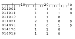
Note 11: Most of the subgrade and base layers use model 1.
For the above example, model 2 (deviator stress model) was found to be a better fit for the subgrade for test section 011021, and the subbase layer (a lime-treated soil) of 014073 was found to be linear.
SENSOR.DAT provides the user an opportunity to change the association of a particular sensor with a particular layer in the pavement system from the default association provided by the program. This may improve the resultant fit and is used more often with nonlinear problems; finding the best association may require several attempts. In addition, this file is used to enter values for layer moduli that the user wishes MODCOMP4 to consider as fixed values, not subject to variation in the calculation. For each layer, input is in the form LL S EEEEE., where LL is the layer number, S is the number of the sensor to be associated with that layer, and EEEEE. is the fixed modulus for that layer. Obviously, if a fixed value is supplied, one should have no sensor associated with that layer.
Because it was desired to be able to associate a sensor with the second (lower) subgrade layer if one was created, for the purposes of this data file, that layer was given an arbitrary designation as layer 10. Because this layer did not exist at the time MODDATA was run, no seed value could then be entered for it; hence, a programming trick allows a seed (NOT a fixed value) to be entered for such a layer if the value of EEEEE. (see above) is negative. Remember that because this file is read into PREMOD3, any modulus values must be in metric units (MPa).
An example of the file follows:
Output files from PREMOD3 are named in such a way as to identify them as well as possible and to avoid duplicate names in a single directory containing as many as 5,000 separate files.
For Seasonal Monitoring Pavement (SMP) sites, the file naming convention is:
ssstttph.dmy
where:
sss = a three-character label for the seasonal site, consisting of the two-digit state code and a letter indicating the specific site within that state, obtained from a data statement within PREMOD3 correlating standard six-character SHRP_ID's to seasonal ID's. These letters are not arbitrary but have been assigned previously.ttt = a three-character label for the station at which the deflections were observed, using M in the first character if the station was negative (no negative three-digit stations were used) and prefixing two- or single-digit stations with 0 and 00, respectively.
p = a single character in alphabetic sequence indicating the number of times the present station and load height have been used so far on this particular day.
l = a single digit (0,1,3) indicating the lane in which the data was taken (0, test pit area; 1, mid-lane; 3, outer wheelpath)
d = a single character (A-Z, 1-5) indicating the day of the month of the site visit.
m = a single character (A-L) indicating the month of the site visit.
y = a single character (0-9) indicating the last digit of the year of the site visit. This convention assumed that all visits were within the same decade, which was true for the present data set.
It should be noted that the pass number p starts at A for a given SHRP_ID, date, and station, and is incremented until either the corresponding file name has not been already used, or 36 values (26 letters + 10 digits) have been attempted, in which case the program prints an error message and quits. A total of 24 cases (corresponding to six sequences of observations and four load heights at each location) should be the maximum needed. Where multiple data sets were taken at the same location on the same sequence, more values may be needed, but this is a data error and should be fixed in the data.
For nonseasonal sites the file-naming convention is:
aaaaaach.lmy
where:
aaaaaa = the full 6-character SHRP_ID of the section being studied.c = a single character (A-Z, 0-9) indicating the station at which the data was taken (for flexible sections, 21 stations are used in each lane, and for rigid sections, up to 20 stations are used for the mid-slab deflections, which are the only ones for which back-calculation is attempted).
h = a single digit (1-4) corresponding to the load height used for the current deflections, corresponding to different nominal loads (6,000; 9,000; 12,000; and 16,000 pounds).
l,m,y = (lane, month, year) as above for seasonal data file names (note that we assume there will not be two visits for non-seasonal sites in the same month, nor will there be more than one complete sequence on a single day).
Step 4: Trial Computations and Modification of Inputs
Execute MODSHELL
To begin the computation process, a limited number of points are manually selected at random along the test section to complete the back-calculation of elastic properties. The number of test points selected are generally in the range of three to eight and depend on the amount of variation of the measured deflection basins within the subsection. For test sections with "uniform" load response, three or four deflection basins should be used, whereas six to eight basins should be used for those test sections with load-response characteristics defined as "drift" or "highly variable."(1)
MODSHELL is used to analyze the basins measured at those random test points. Results from these initial solutions are reviewed to determine whether the production runs should be executed or changes should be made to the inputs before proceeding to the production runs. The decision on whether to proceed is based on, in order of importance:
If the RMS errors are found to be large (greater than 2 percent) or the calculated layer elastic moduli are questionable for the type of material, the inputs should be checked and adjustments made to the layer combinations, layer-sensor assignments, and/or the use or omission of an apparent rigid layer. MODSHELL is used to recalculate the elastic layer modulus with those changes. This iterative process is continued until "reasonable or acceptable" solutions are achieved. As stated above, a reasonable or acceptable solution is one with an RMS error less than or equal to 2 percent with elastic layer moduli that are considered typical for the material type. The revisions, if any, to the input parameters created by PREMOD are then used for the production runs.
For some test sections, extremely high or low layer moduli can be computed for one or more layers in the pavement structure with good RMS error values. If this occurs, changes should be made to the inputs and MODSHELL used to recalculate Young's modulus, as noted above. If the final RMS error is less than 2 percent for the trial runs that resulted in the extremely high or low moduli and is much greater than 2 percent for the other trial runs, the trial run resulting in the high or low moduli should be used for the production runs.
Execute Program BATCHIT
Program BATCHIT creates batch files to assist in the automated handling of the many MODCOMP4 input files generated by PREMOD3. The program is executed from the directory containing those output files (see below). BATCHIT examines the extensions of all the data files; the first batch file creates a subdirectory corresponding to each such extension below a directory specified by the user, and moves all files with that extension to that subdirectory. The second batch file causes the system to change to each of those subdirectories in turn, execute MODCOMP4 on each data file, and compress (using PKZIP) the data files and short and long output files into separate ZIP files for future reference. These ZIP files are stored in <startid>/<stateid>.
The program assumes that the data files from PREMOD3 are in a directory:
<startid>\<stateid>\<seasid>
where:
<startid> = an arbitrary top-level directory.
<stateid> = a subdirectory named using either a two-digit numeric FIPS (Federal Information Processing System) State code (e.g., 01, 48) or a two-character State postal identifier (e.g., AL, TX).<seasid> = in the case of seasonal FWD data this would be the three-character seasonal ID referred to above in the description of PREMOD3 output file names; for nonseasonal data, a three-character substitute was used:
__a, __b, __c, __d, etc.where the a,b,c,d are surrogates for the SHRP_ID's of sections in the current states. It would be possible to modify the program to use the full 6-character ID in this situation, if desired, but some of the later file-naming conventions assume the use of three characters here.
The program requests that the user enter the drive and the value for <startid>.
Examples of the output of BATCHIT for a nonseasonal case (011001, with three-character surrogate __A) follow:
File DO__ADIR.BAT
File DO__AMOD.BAT
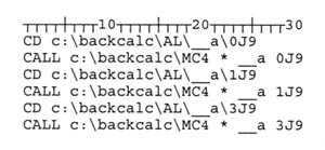
File MC4.BAT
![Line 1: cls; Line 2: REM This batch is called with three arguments:; Line 3: REM 1. The file name part of the file spec (can be wild card [*]); Line 4: REM 2. The seasonal ID for the section under study (e.g., 48E).; Line 5: REM 3. The extension part of the file spec (normally = the DATE code); Line 6: @ECHO OFF; Line 7: BREAK ON; Line 8: FOR %%F IN (%1.%3) DO \MODCOMP4\MODCOMP4 %%F; Line 9: ren *.1st *.out; Line 10: PKZIP -M ..\%2%3SM *.SUM; Line 11: PKZIP -M ..\%2%OT *.OUT; Line 12: PKZIP -M ..\%2%3DT *.%3.](p14.jpg)
Step 5: Execute MODCOMP4 -- Back-Calculate Young's Modulus and Nonlinear Elastic Properties
Program MODCOMP4 is executed for each data file by a call to the separate batch file (MC4.BAT) shown above. It would be impossible to provide an appropriate discussion of this program in this document; it is suggested that the user refer to the documents provided with the MODCOMP4 package.(10)
It is assumed that MODCOMP4.exe is in a directory named MODCOMP4, directly off the current root directory. Upon finishing all of the basins, MC4.BAT also causes the data files, short output files, and long output files to be zipped into files whose names are made up of the seasonal section name or surrogate, therefore, the data file extension (which will be the same for all data files in that directory); and a two-character label (DT, SM, or OT) indicating data, summary or output, respectively. MC4.BAT is assumed to be located in the <startdir> of the discussion for PREMOD3.
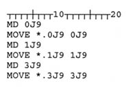
A sample input file for a linear problem (011001A1.0J9, created by PREMOD3) follows:
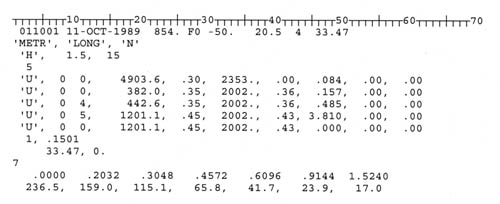
The above file shows the problem identification line, the run parameters, and the fact that there are five layers, each of which is considered to have an unknown modulus. Layers 3 and 4 (counting down from the surface) are to be associated with sensors 4 and 5 (457 and 610 mm from the center of the loading plate). There is one load level, with a load of radius 0.1501 m; the following field (0. in this case) on this line permits specification of load pressure instead of total load). The load is expressed as 33.47 kN, and there are seven sensors, whose positions and readings are given. For each layer, the model is zero (linear), and the initial modulus, Poisson's ratio, density, coefficient of lateral pressure, and thickness are given, followed by zeroes for the estimates of K1 and K2 used for a known layer in a nonlinear solution.
Note 12: The "N" on the end of the second line in the data file is placed there automatically by PREMOD3. It tells MODCOMP4 not to run all load levels for a linear data set; the option of running more than one was added after PREMOD3 was written; hence, no linear data sets are written with more than one load level.
Step 6: Extract Elastic Properties and Create Summary Output Files
Execute BACKSUM2
Program BACKSUM2 is run to obtain summary information from the MODCOMP4 summary (short) output files for the final iteration of linear back-calculation runs. The data desired are the SHRP_ID, the date, time, and temperature when the deflections were obtained, the location (station and lane), the load applied, the thickness and derived modulus for each layer, and the average error between the observed and predicted deflections for the final values of layer modulus. The program is run from the directory containing the ZIP files created by the second batch file and expands each SM (summary) ZIP file, obtains a directory of the summary files, and extracts the required information from each file in turn.
The output for all of the summary files in a given ZIP file is written to a single file, one line per basin, whose location in the directory structure is given by a file DIRECT.NAM in the current directory and whose file name is the first six characters of the ZIP file, which is made up of the three-character seasonal ID (or its surrogate for nonseasonal sections) and the three-character data file extension. If DIRECT.NAM does not exist, the user is prompted for the need to create it, and the program is halted. The program could be modified to assume that the file DIRECT.NAM is in a standard location, instead of being in the current directory. Sample output follows:
Execute BAKSUMNL
Program BAKSUMNL does what BACKSUM2 does but for the results of nonlinear calculations. The MODCOMP4 output formats are slightly different, and the results in terms of layer modulus are given only for the highest load value for which a basin was included (remember that for nonlinear processing, the MODCOMP4 data files each contain the basins for a full four load levels done at that time and place). Sample output follows:
Note that layer 1 is linear (L), the nonlinear solution for layers 2,3, and 4 is sometimes significant (S) and sometimes not (N), and layer 5 has fixed modulus (F). TAC is the asphalt mid-depth temperature, MOD is the model number assumed for the layer, and #DRP is the number of drops included in the averaged basin. Note also that, at station 400, the MODCOMP4 solution ran out of iterations before converging.
Execute BAKOUTNL
Program BAKOUTNL operates on the longer output files for nonlinear back-calculation results to obtain information not available from the shorter summary output files. Specifically, BAKOUTNL obtains, in addition to necessary identification information, the coefficients and exponents in the mathematical relation assumed by the user to hold for the particular layer material.
In addition the number of the model used, Poisson's ratio, the coefficient of lateral pressure, and the density of the layer are extracted, as well as the correlation coefficient R for the regression between modulus and stress for the different load levels, showing how well the chosen model actually fits the data.
Note 13: The number obtained is R, not the R-squared that is usually used in this application.
If a linear layer is included in the layer structure, the modulus obtained for that layer under the highest load is retrieved instead of the model parameters.
The program is executed for each nonlinear back-calculation, with two parameters, as shown below:
BAKOUTNL <infile> <outfile>
where <infile> is a long output file of MODCOMP4, and the output is written to <outfile> as one line per layer. Sample output follows:
Note here, for the example, that COEFF and EXP are 0.0 for the linear asphalt layer and the fixed layer.
Summary
This guide has been prepared to implement and apply existing standardized procedures (ASTM D5858 and FHWA-RD-97-076) to back-calculate Young's modulus and the nonlinear elastic properties for each pavement and subgrade layer.(1) However, the use of MODCOMP4, as well as other software packages, to calculate elastic layer properties from FWD deflection basins does not always provide reasonable solutions, because the program is not a perfect simulation of real-world conditions. Each program has limitations and inaccuracies in simulating the deflection basins.
Appendix B provides a listing of the LTPP test sections that have extensive variability and drift and those that were subdivided into two subsections. Appendix B also provides a listing of the LTPP test sections where an apparent rigid layer was used in the back-calculation process and the depth to sampling refusal from the shoulder probe drilled at each site.
| Consistent Change in Deflections Along the Test Section -- "Drift" (figure 11) | Highly Variable Deflections Along the Test Section (figure 10) | Abrupt Change in Deflections Along the Test Section (figure 12) |
|---|---|---|
| 02 - 1004 | 04 - 1007 | 01 - 4127 --- 2+75* |
| 02 - 6010 | 04 - 1016 | 01 - 4129 --- 2+75 |
| 04 - 1021 | 04 - 1025 | 02 - 9035 --- 2+25 |
| 04 - 1065 | 04 - 6054 | 02 - 1001 --- 2+75 |
| 06 - 8149 | 04 - 6055 | 04 - 1018 --- 0+75 |
| 06 - 8156 | 04 - 6060 | 04 - 1002 --- 1+50 |
| 08 - 2008 | 05 - 2042 | 04 - 1034 --- 1+75 |
| 08 - 7780 | 06 - 2002 | 04 - 1065 --- 2+25 |
| 13 - 4111 | 06 - 2004 | 04 - 1022 --- 2+50 |
| 15 - 1003 | 06 - 2040 | 04 - 1037 --- 2+50 |
| 16 - 1007 | 06 - 2041 | 04 - 1015 --- 2+75 |
| 16 - 9032 | 06 - 2053 | 04 - 1006 --- 3+25 |
| 17 - 9327 | 06 - 8201 | 04 - 1016 --- 2+50 |
| 21 - 1010 | 06 - 8202 | 04 - 6053 --- 2+75 |
| 21 - 6040 | 08 - 1057 | 06 - 8534 --- 3+00 |
| 26 - 1001 | 08 - 7781 | 08 - 6002 --- 3+25 |
| 27 - 1087 | 13 - 1001 | 08 - 6013 --- 1+75 |
| 28 - 3083 | 15 - 7080 | 19 - 6049 --- 3+25 |
| 30 - 7088 | 19 - 1044 | 20 - 1005 --- 1+25 |
| 34 - 1031 | 19 - 6150 | 20 - 7085 --- 2+75 |
| 37 - 1803 | 27 - 1085 | 21 - 6043 --- 3+75 |
| 37 - 1814 | 27 - 7090 | 27 - 1023 --- 2+25 |
| 37 - 2819 | 28 - 2807 | 27 - 1087 --- 1+75 |
| 37 - 2824 | 28 - 3082 | 27 - 1029 --- 0+75 |
| 38 - 2001 | 28 - 3085 | 30 - 7088 --- 1+75 |
| 40 - 1017 | 28 - 3089 | 31 - 6702 --- 0+25 |
| 40 - 6010 | 28 - 7012 | 37 - 1992 --- 1+75 |
| 42 - 1618 | 29 - 1010 | 37 - 2824 --- 2+75 |
| 45 - 1025 | 29 - 5403 | 38 - 2001 --- 2+50 |
| 47 - 3075 | 29 - 5413 | 40 - 4088 --- 1+50 |
| 48 - 1039 | 30 - 7076 | 41 - 6012 --- 3+50 |
| 48 - 1076 | 31 - 6700 | 42 - 1614 --- 2+25 |
| 48 - 1174 | 31 - 7040 | 42 - 1618 --- 3+75 |
| 49 - 1007 | 32 - 1020 | 45 - 1011 --- 1+25 |
| 49 - 1017 | 32 - 1021 | 47 - 3110 --- 3+00 |
| 51 - 1002 | 35 - 1002 | 48 - 1061 --- 4+25 |
| 51 - 1417 | 35 - 6033 | 48 - 1096 --- 3+00 |
| 51 - 1464 | 36 - 1011 | 48 - 3669 --- 1+00 |
| 51 - 2021 | 37 - 1024 | 48 - 9005 --- 2+25 |
| 81 - 1804 | 37 - 1040 | 49 - 1004 --- 2+25 |
| 37 - 1801 | 53 - 1002 --- 3+25 | |
| 37 - 1802 | 53 - 6056 --- 1+00 | |
| 37 - 1817 | 56 - 2015 --- 2+25 | |
| 37 - 2825 | 56 - 7772 --- 1+25 | |
| 40 - 4087 | 81 - 1805 --- 3+50 | |
| 41 - 2002 | 81 - 2812 --- 2+25 | |
| 42 - 7025 | ||
| 45 - 1008 | ||
| 45 - 7019 | ||
| 46 - 9106 | ||
| 47 - 3101 | ||
| 47 - 3104 | ||
| 47 - 6022 | ||
| 47 - 9025 | ||
| 48 - 1050 | ||
| 48 - 1056 | ||
| 48 - 1094 | ||
| 48 - 1109 | ||
| 48 - 1111 | ||
| 48 - 1119 | ||
| 48 - 1168 | ||
| 48 - 1181 | ||
| 48 - 1183 | ||
| 48 - 2176 | ||
| 48 - 3609 | ||
| 48 - 3679 | ||
| 48 - 3689 | ||
| 48 - 3769 | ||
| 48 - 3865 | ||
| 48 - 6079 | ||
| 48 - 6160 | ||
| 49 - 1008 | ||
| 50 - 1682 | ||
| 51 - 1423 | ||
| 51 - 2004 | ||
| 53 - 1008 | ||
| 53 - 1501 | ||
| 56 - 2017 | ||
| 56 - 2018 | ||
| 82 - 6006 | ||
| 87 - 1620 | ||
| 87 - 2812 | ||
| 90 - 6420 |
| State Code | LTPP Test Section Identification Number | Average Depth to an Apparent Rigid Layer, m | Refusal Depth Noted on Boring Log, m |
|---|---|---|---|
| 01 | 1019 | 6.4 | 7.5 |
| 01 | 4126 | 3.4 | |
| 01 | 6019 | 7.6 | |
| 01 | B330 | 6.4 | 6.2 |
| 02 | 1008 | 7.6 | |
| 02 | 6010 | 4.5 | |
| 04 | 0113 | 7.6 | |
| 04 | 0114 | 7.6 | |
| 04 | 0606 | 1.8 | |
| 04 | 1007 | 6.1 | |
| 04 | 0115 | 15.2 | |
| 04 | 0116 | 15.2 | 3.3 |
| 04 | 0117 | 15.2 | |
| 04 | 0118 | 15.2 | |
| 04 | 0119 | 15.2 | |
| 04 | 0120 | 15.2 | |
| 04 | 0121 | 15.2 | |
| 04 | 0122 | 15.2 | |
| 04 | 0123 | 15.2 | |
| 04 | 0124 | 15.2 | |
| 04 | 1016 | 15.2 | |
| 04 | 1018 | 15.2 | |
| 04 | 1025 | 2.0 | 2.1 |
| 04 | 1034 | 6.1 | |
| 04 | 1003 | 15.2 | |
| 04 | 1037 | 6.7 | |
| 04 | 1062 | 7.6 | 1.4 |
| 04 | 1065 | 7.6 | |
| 04 | 6053 | 15.2 | |
| 04 | 6054 | 15.2 | |
| 04 | 6055 | 15.2 | |
| 04 | 6060 | 7.6 | |
| 04 | D320 | 15.2 | |
| 04 | D330 | 15.1 | |
| 04 | 7613 | 3.2 | |
| 05 | 2042 | 2.4 | |
| 05 | 5805 | 0.9 | |
| 05 | 0213 | 0.7 | |
| 05 | 0214 | 3.7 | |
| 05 | 0217 | 3.4 | |
| 05 | 0218 | 3.2 | |
| 05 | 0221 | 2.1 | |
| 06 | 2002 | 7.6 | 0.4 |
| 06 | 2004 | 7.6 | |
| 06 | 2040 | 15.2 | |
| 06 | 2053 | 15.2 | |
| 06 | 6044 | 15.2 | |
| 06 | 7452 | 7.6 | |
| 06 | 7454 | 15.2 | |
| 06 | 8149 | 7.6 | |
| 06 | 8153 | 15.2 | |
| 06 | 8156 | 15.2 | |
| 06 | 8202 | 15.2 | |
| 06 | 8534 | 7.6 | |
| 06 | 8535 | 7.6 | |
| 06 | 2051 | 0.9 | |
| 06 | 3010 | 1.8 | |
| 06 | 3021 | 2.7 | |
| 06 | 8151 | 2.4 | |
| 06 | 8201 | 4.0 | |
| 06 | A320 | 7.6 | |
| 06 | A330 | 7.6 | |
| 06 | A350 | 1.1 | |
| 08 | 1047 | 15.2 | |
| 08 | 2008 | 1.2 | |
| 08 | 6013 | 15.2 | |
| 08 | 7036 | 15.2 | |
| 08 | 7780 | 15.2 | |
| 08 | 7781 | 6.4 | |
| 08 | 7783 | 1.0 | |
| 08 | 3032 | 1.6 | |
| 09 | 1803 | 1.2 | |
| 12 | 1030 | 15.2 | |
| 12 | 4096 | 15.2 | |
| 12 | 4106 | 6.0 | |
| 12 | 4108 | 15.2 | |
| 12 | 4153 | 8.0 | |
| 12 | 4154 | 5.7 | |
| 12 | A330 | 7.6 | |
| 12 | 0101 | 1.7 | |
| 12 | 0102 | 2.0 | |
| 12 | 0103 | 2.2 | |
| 12 | 0104 | 2.2 | |
| 12 | 0105 | 1.6 | |
| 12 | 0106 | 2.2 | |
| 12 | 0107 | 2.7 | |
| 12 | 0108 | 2.3 | |
| 12 | 0109 | 2.1 | |
| 12 | 0110 | 2.0 | |
| 12 | 0111 | 1.9 | |
| 12 | 0112 | 2.3 | |
| 13 | 0502 | 3.7 | |
| 13 | 0503 | 5.9 | |
| 13 | 0506 | 1.8 | |
| 13 | 1031 | 15.2 | |
| 13 | 3016 | 1.5 | |
| 13 | 3017 | 3.7 | |
| 13 | 4092 | 5.4 | |
| 13 | 4111 | 3.6 | |
| 13 | 4112 | 5.1 | |
| 13 | 4113 | 15.2 | |
| 13 | 4420 | 15.2 | |
| 13 | 7028 | 15.2 | |
| 15 | 1003 | 1.8 | |
| 15 | 1006 | 15.2 | |
| 16 | 1001 | 2.2 | 1.2 |
| 16 | 1007 | 15.2 | 1.8 |
| 16 | A320 | 3.0 | |
| 16 | A330 | 3.0 | |
| 16 | A350 | 3.0 | |
| 16 | 1005 | 1.8 | |
| 16 | 1020 | 3.0 | |
| 16 | 1021 | 0.8 | |
| 16 | 5025 | 3.7 | |
| 16 | 6027 | 2.0 | |
| 17 | 1002 | 15.1 | |
| 17 | 5423 | 15.2 | |
| 17 | 5453 | 15.2 | |
| 17 | 6050 | 15.2 | |
| 17 | 7937 | 15.2 | |
| 18 | 1028 | 3.6 | |
| 18 | 1037 | 15.2 | |
| 18 | 6012 | 5.1 | |
| 19 | 6150 | 7.6 | |
| 20 | 7073 | 15.2 | |
| 20 | 1005 | 4.9 | |
| 20 | 1006 | 4.9 | |
| 20 | 3013 | 3.8 | |
| 20 | 4053 | 3.8 | |
| 21 | 1014 | 6.1 | |
| 21 | 6040 | 2.6 | 2.6 |
| 21 | 1010 | 4.6 | |
| 21 | 1034 | 3.0 | |
| 21 | 4025 | 1.6 | |
| 22 | 3056 | 15.2 | |
| 23 | 1001 | 15.1 | 2.0 |
| 23 | 1009 | 2.3 | |
| 23 | 1012 | 3.7 | |
| 23 | 1028 | 15.2 | |
| 23 | 7023 | 5.5 | |
| 23 | 3013 | 2.3 | |
| 24 | 0503 | 2.0 | |
| 24 | 2805 | 1.1 | |
| 25 | 1003 | 3.1 | |
| 25 | 1004 | 3.1 | |
| 26 | 1001 | 15.1 | |
| 26 | 1012 | 2.5 | |
| 26 | 7072 | 15.2 | |
| 26 | 1004 | 2.2 | |
| 27 | 1016 | 3.3 | |
| 27 | 1018 | 2.3 | |
| 27 | 1087 | 15.2 | |
| 27 | 6251 | 2.8 | |
| 27 | 7090 | 15.2 | |
| 27 | D330 | 4.0 | |
| 27 | D340 | 4.0 | |
| 28 | 2807 | 15.2 | |
| 28 | 3081 | 15.2 | |
| 28 | 3082 | 15.2 | |
| 28 | 3083 | 4.2 | |
| 28 | 3089 | 15.2 | |
| 28 | 3090 | 15.2 | |
| 29 | 1005 | 15.2 | |
| 29 | 1008 | 15.2 | |
| 29 | 7054 | 15.2 | |
| 29 | 7073 | 15.2 | |
| 29 | 0707 | 0.9 | |
| 29 | 0709 | 1.0 | |
| 29 | 1010 | 2.3 | |
| 29 | 4036 | 1.5 | |
| 29 | 5473 | 0.6 | |
| 30 | 0506 | 15.2 | |
| 30 | 0507 | 15.2 | 5.9 |
| 30 | 0509 | 15.2 | |
| 31 | 0120 | 15.2 | |
| 31 | 0121 | 15.2 | |
| 31 | 7005 | 15.2 | |
| 31 | 7017 | 15.2 | |
| 31 | 7040 | 15.2 | |
| 31 | 7050 | 15.2 | |
| 32 | 1020 | 7.6 | |
| 32 | 7000 | 6.1 | |
| 32 | A310 | 5.9 | |
| 32 | A320 | 5.9 | |
| 32 | A330 | 5.9 | |
| 32 | A350 | 5.9 | |
| 32 | B310 | 6.1 | |
| 32 | B320 | 6.1 | |
| 32 | B340 | 6.1 | |
| 32 | B350 | 6.1 | |
| 32 | 1030 | 1.5 | |
| 34 | 1003 | 15.2 | 1.4 |
| 34 | 1011 | 2.8 | |
| 34 | 1030 | 1.4 | 1.4 |
| 34 | 1033 | 2.6 | 3.0 |
| 34 | 1034 | 15.2 | |
| 34 | 1638 | 15.2 | |
| 34 | 6057 | 15.2 | 4.4 |
| 35 | 6033 | 7.6 | |
| 35 | 6035 | 7.6 | |
| 35 | 6401 | 7.6 | |
| 35 | 0107 | 3.4 | |
| 35 | 1002 | 0.5 | |
| 35 | 1003 | 0.9 | |
| 35 | 2118 | 5.3 | |
| 35 | 3010 | 5.0 | |
| 36 | A310 | 15.2 | |
| 36 | A320 | 15.2 | |
| 36 | A340 | 15.2 | |
| 36 | A350 | 15.2 | |
| 36 | B310 | 1.5 | |
| 36 | B340 | 1.5 | |
| 36 | 0801 | 4.3 | |
| 36 | 0802 | 3.7 | |
| 36 | 1644 | 1.5 | |
| 37 | 1006 | 15.2 | |
| 37 | 1645 | 15.2 | |
| 37 | 1814 | 4.1 | 4.1 |
| 37 | 1024 | 1.4 | |
| 37 | 1803 | 1.1 | |
| 37 | 2824 | 1.4 | |
| 37 | 3044 | 5.5 | |
| 38 | 2001 | 15.2 | |
| 39 | 7021 | 15.2 | |
| 39 | 0208 | 6.1 | |
| 39 | 3801 | 2.7 | |
| 40 | 4154 | 15.2 | |
| 40 | 6010 | 4.9 | 4.9 |
| 40 | 7024 | 1.8 | 1.8 |
| 40 | A320 | 5.0 | |
| 40 | A340 | 5.0 | |
| 40 | A350 | 5.0 | |
| 40 | 4157 | 1.4 | |
| 40 | 0113 | 4.1 | |
| 40 | 0114 | 0.2 | |
| 40 | 0115 | 3.7 | |
| 40 | 0116 | 0.9 | |
| 40 | 0117 | 1.8 | |
| 40 | 0118 | 1.2 | |
| 40 | 0119 | 1.8 | |
| 40 | 0120 | 2.7 | |
| 40 | 0121 | 1.2 | |
| 40 | 0122 | 0.8 | |
| 40 | 0123 | 0.9 | |
| 40 | 0124 | 5.2 | |
| 42 | 1599 | 7.6 | 2.3 |
| 42 | 1605 | 7.6 | |
| 42 | 1608 | 7.6 | |
| 42 | 1610 | 15.2 | |
| 42 | 1618 | 7.6 | 5.2 |
| 42 | 7025 | 1.7 | 2.3 |
| 42 | 7037 | 15.2 | |
| 42 | A310 | 15.2 | |
| 42 | A320 | 15.2 | |
| 42 | A330 | 15.2 | |
| 42 | A340 | 15.2 | |
| 42 | A350 | 15.2 | |
| 42 | B310 | 15.2 | |
| 42 | B330 | 15.2 | |
| 42 | B350 | 15.2 | |
| 42 | 0601 | 2.7 | |
| 42 | 0602 | 3.0 | |
| 42 | 0605 | 2.9 | |
| 42 | 0607 | 2.4 | |
| 42 | 1598 | 1.0 | |
| 42 | 1606 | 5.1 | |
| 42 | 1613 | 2.7 | |
| 42 | 9027 | 2.6 | |
| 44 | 7401 | 4.6 | |
| 45 | 1008 | 2.6 | |
| 45 | 7019 | 3.7 | |
| 45 | 3012 | 3.4 | |
| 46 | 3013 | 1.8 | |
| 46 | 3053 | 1.2 | |
| 46 | 5020 | 1.8 | |
| 46 | 9187 | 5.0 | |
| 46 | 9197 | 2.1 | |
| 47 | 1029 | 7.6 | |
| 47 | 2001 | 3.8 | |
| 47 | 2008 | 15.2 | |
| 47 | 3075 | 5.9 | |
| 47 | 3104 | 7.6 | 2.7 |
| 47 | A310 | 3.7 | |
| 47 | A320 | 3.7 | |
| 47 | A330 | 3.7 | |
| 47 | A350 | 3.7 | |
| 47 | 3101 | 3.7 | |
| 47 | 3108 | 5.6 | |
| 47 | 3109 | 1.5 | |
| 47 | 9024 | 3.4 | |
| 48 | 0001 | 7.6 | |
| 48 | 1046 | 15.2 | |
| 48 | 1047 | 7.6 | |
| 48 | 1048 | 6.3 | |
| 48 | 1049 | 3.3 | |
| 48 | 1060 | 15.2 | |
| 48 | 1061 | 7.6 | |
| 48 | 1069 | 15.2 | |
| 48 | 1070 | 15.2 | |
| 48 | 1077 | 15.2 | |
| 48 | 1094 | 7.6 | |
| 48 | 1116 | 1.2 | |
| 48 | 1130 | 15.2 | |
| 48 | 1168 | 7.6 | |
| 48 | 1169 | 6.1 | |
| 48 | 1181 | 3.9 | |
| 48 | 2172 | 15.2 | 3.4 |
| 48 | 2176 | 15.2 | |
| 48 | 3629 | 7.6 | |
| 48 | 3669 | 15.2 | |
| 48 | 3679 | 10.9 | |
| 48 | 3729 | 15.2 | |
| 48 | 3855 | 7.6 | |
| 48 | 3865 | 5.6 | 5.0 |
| 48 | 6086 | 15.1 | |
| 48 | 6160 | 7.6 | |
| 48 | 6179 | 2.2 | |
| 48 | 7165 | 15.2 | |
| 48 | 9005 | 7.6 | |
| 48 | B330 | 15.2 | |
| 48 | D330 | 15.2 | |
| 48 | 3845 | 4.4 | |
| 48 | 5035 | 2.4 | |
| 48 | 5278 | 0.6 | |
| 48 | 5301 | 1.8 | |
| 48 | 9355 | 2.4 | |
| 49 | 1004 | 2.4 | |
| 49 | 1005 | 15.2 | |
| 49 | 1006 | 6.1 | |
| 49 | 1007 | 15.2 | 3.0 |
| 49 | 1017 | 6.3 | |
| 49 | 0803 | 2.1 | |
| 49 | 0804 | 1.8 | |
| 50 | 1004 | 15.2 | |
| 50 | 1681 | 15.2 | |
| 50 | 1683 | 3.8 | |
| 51 | 1023 | 15.2 | |
| 51 | 1464 | 7.6 | |
| 51 | 2004 | 15.2 | |
| 51 | 2021 | 5.0 | 1.1 |
| 51 | 1002 | 1.8 | |
| 51 | 1419 | 3.7 | |
| 51 | 1423 | 1.2 | |
| 51 | 0116 | 2.4 | |
| 51 | 0117 | 1.1 | |
| 51 | 0121 | 2.1 | |
| 51 | 0122 | 0.9 | |
| 51 | 0123 | 2.3 | |
| 53 | 1008 | 15.2 | |
| 53 | 1501 | 7.6 | 1.7 |
| 53 | 1801 | 7.6 | 1.1 |
| 53 | 1002 | 1.7 | |
| 53 | 3813 | 1.8 | |
| 53 | 6020 | 2.3 | |
| 53 | 6049 | 4.3 | |
| 53 | 7409 | 0.8 | |
| 53 | 0201 | 3.4 | |
| 53 | 0202 | 0.3 | |
| 53 | 0203 | 0.7 | |
| 53 | 0204 | 1.7 | |
| 53 | 0206 | 2.7 | |
| 53 | 0208 | 1.2 | |
| 53 | 0209 | 0.4 | |
| 53 | 0210 | 0.8 | |
| 53 | 0211 | 0.8 | |
| 53 | 0212 | 0.4 | |
| 54 | 1640 | 2.1 | 2.1 |
| 54 | 7008 | 15.2 | |
| 54 | 4003 | 2.1 | |
| 54 | 4004 | 2.1 | |
| 54 | 5007 | 2.1 | |
| 55 | 6351 | 1.8 | |
| 55 | 6352 | 1.2 | |
| 55 | 6354 | 2.7 | |
| 55 | 6355 | 2.1 | |
| 56 | 2015 | 7.6 | |
| 56 | 2019 | 15.2 | |
| 56 | 2020 | 15.2 | |
| 56 | 6029 | 2.5 | |
| 56 | A330 | 6.1 | |
| 56 | 2018 | 5.3 | |
| 56 | 6032 | 0.9 | |
| 56 | 7775 | 3.0 | |
| 72 | 4121 | 1.8 | |
| 81 | 1804 | 9.3 | |
| 81 | 8529 | 1.5 | |
| 82 | 1005 | 5.5 | |
| 82 | 6006 | 6.4 | |
| 82 | 6007 | 3.3 | |
| 83 | 6454 | 15.2 | |
| 84 | 1684 | 7.6 | |
| 84 | 1802 | 7.6 | |
| 84 | 6804 | 6.1 | |
| 84 | 3803 | 5.8 | |
| 85 | 1801 | 7.6 | 1.4 |
| 85 | 1803 | 6.1 | 0.9 |
| 85 | 1808 | 7.6 | 0.8 |
| 86 | 6802 | 7.6 | 1.3 |
| 87 | 1620 | 7.6 | |
| 87 | 1680 | 3.2 | |
| 87 | 1806 | 2.2 | |
| 87 | A310 | 15.2 | |
| 88 | 1645 | 7.6 | |
| 88 | 1646 | 7.6 | |
| 88 | 1647 | 7.6 | |
| 89 | 1021 | 15.2 | |
| 89 | 1125 | 15.2 | |
| 89 | 1127 | 15.2 | |
| 89 | 2011 | 15.1 | |
| 89 | A310 | 15.2 | |
| 89 | A320 | 7.6 | |
| 89 | A330 | 7.6 | |
| 89 | A340 | 7.6 | |
| 89 | 9018 | 5.6 | |
| 89 | A901 | 1.8 | |
| 89 | A902 | 1.3 | |
| 90 | 6400 | 3.3 | |
| 90 | 6801 | 3.3 |
| State Code | SHRP Identification Number | Test Date with Non-Standard Sensor Placement |
|---|---|---|
| 5 | 0902 | 9-11-96 |
| 5 | 0902 | 9-12-96 |
| 5 | 0903 | 9-11-96 |
| 5 | A601 | 9-13-96 |
| 5 | A602 | 9-14-96 |
| 5 | A603 | 9-13-96 |
| 5 | A606 | 9-12-96 |
| 5 | A606 | 9-13-96 |
| 5 | A608 | 9-12-96 |
| 28 | 0805 | 9-17-96 |
| 28 | 0806 | 9-17-96 |
| 28 | 0902 | 9-18-96 |
| 28 | 0903 | 9-18-96 |
| 28 | 0959 | 9-18-96 |
| 47 | 3104 | 10-25-96 |
| 48 | 1092 | 6-29-96 |
| 48 | 1094 | 7-30-96 |
| 48 | 1096 | 7-29-96 |
| 48 | 1109 | 8-5-96 |
| 48 | 1122 | 8-1-96 |
| 48 | 3589 | 9-5-96 |
| 48 | 3845 | 8-22-96 |
| 48 | 5328 | 8-23-96 |
| 48 | 9005 | 7-31-96 |
| 48 | A310 | 7-30-96 |
| 48 | A320 | 7-30-96 |
| 48 | A330 | 7-30-96 |
| 48 | A340 | 7-30-96 |
| 48 | A350 | 7-30-96 |
| 48 | C410 | 8-21-96 |
| 48 | C420 | 8-21-96 |
| 48 | C420 | 9-4-96 |
| 48 | C430 | 9-4-96 |
| 48 | J310 | 8-1-96 |
| 48 | J320 | 8-1-96 |
| 48 | J330 | 8-1-96 |
| 48 | J340 | 8-1-96 |
| 48 | J350 | 8-1-96 |
| 48 | K310 | 7-31-96 |
| 48 | K320 | 7-31-96 |
| 48 | K330 | 7-31-96 |
| 48 | K340 | 8-2-96 |
| 48 | K350 | 8-2-96 |
| 48 | K351 | 7-31-96 |
Appendix C is a summary of the results from the back-calculation of elastic properties. It is subdivided into two basic parts. The first part is a tabulation of the test sections for which only a few of the deflection basins (less than 30 percent) had solutions with RMS errors less than 2 percent and the median Young's modulus for different materials and pavement cross-sections for those solutions with RMS errors of less than 2 percent. The second part includes histograms of the results from the back-calculation of Young's modulus for different pavement materials and soils.
| State Code | LTPP Test Section Identification Number | Number of Basins | Percentage of Basins with an RMS Error of Less than 2 Percent |
|---|---|---|---|
| 04 | 0116 | 264 | 19.7 |
| 04 | D320 | 48 | 2.1 |
| 04 | D330 | 48 | 16.7 |
| 06 | A350 | 107 | 27.1 |
| 12 | A330 | 143 | 11.2 |
| 12 | C350 | 48 | 8.3 |
| 16 | A320 | 36 | 16.7 |
| 16 | A350 | 36 | 16.7 |
| 30 | 0509 | 136 | 14.7 |
| 40 | B350 | 48 | 18.8 |
| 56 | A330 | 140 | 17.9 |
| 81 | 0506 | 48 | 20.8 |
| 83 | 0502 | 164 | 11.0 |
| 83 | 0503 | 160 | 27.5 |
| 83 | 1801 | 2741 | 24.3 |
| 02 | 6010 | 591 | 10.7 |
| 02 | 9035 | 156 | 12.2 |
| 04 | 1002 | 511 | 15.3 |
| 04 | 1015 | 344 | 17.4 |
| 04 | 1017 | 1340 | 11.7 |
| 04 | 1018 | 564 | 00.4 |
| 04 | 1025 | 556 | 21.8 |
| 04 | 1037 | 512 | 26.0 |
| 04 | 6054 | 300 | 26.0 |
| 04 | 6055 | 344 | 14.5 |
| 04 | 6060 | 348 | 10.6 |
| 06 | 2053 | 167 | 28.7 |
| 06 | 8149 | 336 | 21.4 |
| 08 | 2008 | 679 | 25.5 |
| 08 | 7783 | 344 | 15.7 |
| 12 | 4103 | 320 | 8.4 |
| 12 | 4135 | 336 | 00.3 |
| 12 | 4137 | 327 | 27.8 |
| 12 | 4153 | 340 | 6.5 |
| 12 | 4154 | 629 | 15.9 |
| 12 | 9054 | 388 | 21.1 |
| 13 | 4093 | 504 | 29.0 |
| 16 | 1001 | 340 | 23.8 |
| 16 | 1021 | 428 | 20.0 |
| 16 | 6027 | 176 | 00.6 |
| 18 | 1028 | 930 | 28.4 |
| 21 | 1034 | 583 | 28.1 |
| 26 | 1010 | 596 | 17.3 |
| 27 | 1016 | 764 | 11.3 |
| 28 | 3085 | 344 | 20.1 |
| 30 | 1001 | 508 | 00.2 |
| 30 | 6004 | 344 | 00.3 |
| 30 | 7075 | 344 | 21.5 |
| 30 | 7088 | 344 | 21.5 |
| 32 | 7000 | 344 | 6.1 |
| 37 | 1992 | 168 | 13.7 |
| 37 | 2819 | 331 | 22.7 |
| 45 | 1008 | 330 | 2.7 |
| 45 | 1024 | 427 | 11.2 |
| 46 | 9197 | 176 | 13.1 |
| 47 | 1028 | 516 | 20.7 |
| 47 | 3104 | 432 | 18.3 |
| 48 | 1061 | 176 | 13.1 |
| 48 | 1168 | 344 | 12.2 |
| 48 | 1169 | 272 | 15.4 |
| 48 | 3579 | 436 | 6.7 |
| 48 | 3855 | 328 | 00.3 |
| 49 | 1004 | 340 | 4.1 |
| 49 | 1005 | 344 | 4.4 |
| 49 | 1007 | 340 | 9.4 |
| 49 | 1008 | 344 | 22.1 |
| 49 | 1017 | 344 | 19.5 |
| 53 | 1008 | 932 | 14.5 |
| 53 | 1501 | 628 | 6.4 |
| 56 | 2015 | 176 | 9.1 |
| 56 | 2037 | 173 | 11.6 |
| 56 | 6029 | 344 | 00.3 |
| 56 | 7772 | 343 | 17.5 |
| Material | Number of Test Points | Median Young's Modulus, MPa |
|---|---|---|
| AASHTO Soil Classification A-1-a | 2,106 | 184 |
| AASHTO Soil Classification A-1-b | 1,128 | 383 |
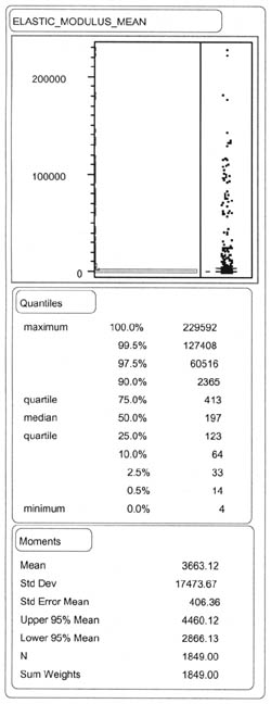
| AASHTO Soil Classification A-2-4 | 1,849 | 197 |
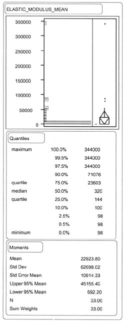
| AASHTO Soil Classification A-2-5 | 33 | 320 |
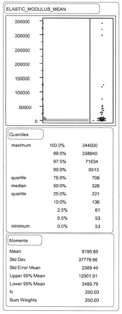
| AASHTO Soil Classification A-2-6 | 250 | 328 |
| AASHTO Soil Classification A-2-7 | 21 | 702 |
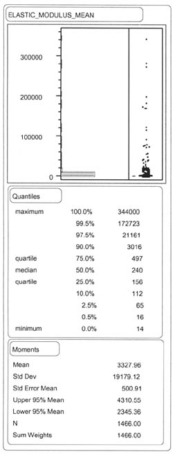
| AASHTO Soil Classification A-3 | 1,466 | 240 |
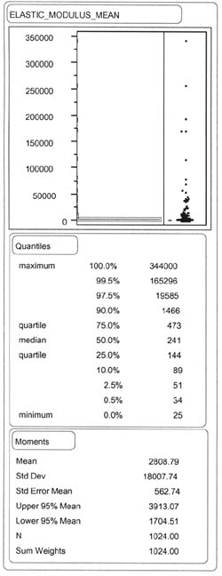
| AASHTO Soil Classification A-4 | 1,024 | 241 |
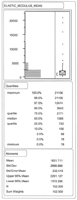
| AASHTO Soil Classification A-5 | 152 | 1,069 |
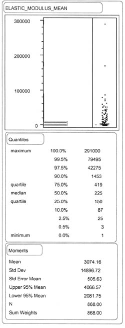
| AASHTO Soil Classification A-6 | 868 | 225 |
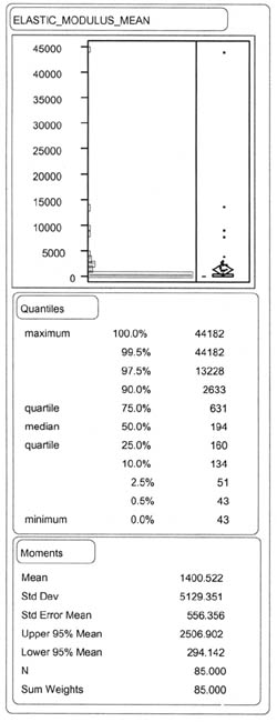
| AASHTO Soil Classification A-7-5 | 85 | 194 |
| AASHTO Soil Classification A-7-6 | 422 | 158 |
| Aggregate Base and Subbase Layers Granular Base Materials | 1,564 | 193 |
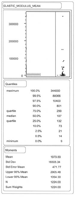
| Aggregate Base and Subbase Layers Granular Materials, Undefined | 1,224 | 187 |
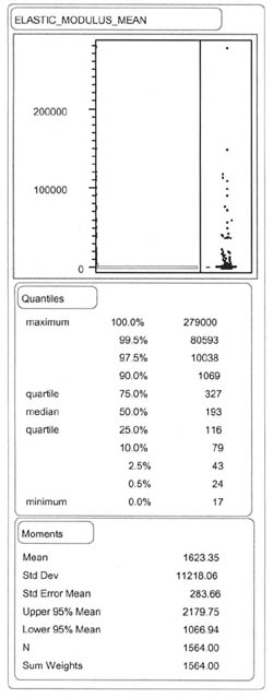
| Aggregate Base and Subbase Layers Granular Subbase Materials | 710 | 152 |
| Asphalt-Treated Base Flexible pavements | 1,923 | |
| Asphalt-Treated Base Rigid pavements | 1,580 | |
| Asphalt-Treated Base Semirigid | 6,407 | |
| Cement-Treated Base Flexible pavements | 5,352 | |
| Cement-Treated Base Rigid pavements | 3,110 | |
| Cement-Treated Base Semi-rigid | 1,332 | |
| HMA, Flexible Pavements Temp. = Cold | 10,229 | |
| HMA, Flexible Pavements Temp. = Moderate | 8,102 | |
| HMA, Flexible Pavements Temp. = Hot | 4,902 | |
| HMA, Rigid Pavements Temp. = Cold | 5,940 | |
| HMA, Rigid Pavements Temp. = Moderate | 5,470 | |
| HMA, Rigid Pavements Temp. = Hot | 3,350 | |
| HMA, Semi-rigid Pavement Temp. = Cold | 15,899 | |
| HMA, Semi-rigid Pavement Temp. = Moderate | 9,557 | |
| HMA, Semi-rigid Pavement Temp. = Hot | 5,242 |
| Temperature Range, Degrees C | Number of Test Points | Average Temperature, Degrees C | HMA Young's Modulus, MPa |
|---|---|---|---|
| -20 to -15 | 9 | -17.5 | 70,372 |
| -15 to -10 | 19 | -13.3 | 71,927 |
| -10 to -5 | 35 | -7.1 | 49,250 |
| -5 to 0 | 141 | -1.6 | 28,802 |
| 0 to 5 | 315 | 2.9 | 15,063 |
| 5 to 10 | 683 | 7.9 | 12,745 |
| 10 to 15 | 1,047 | 12.8 | 11,354 |
| 15 to 20 | 1,135 | 17.4 | 11,639 |
| 20 to 25 | 1,178 | 22.5 | 9,518 |
| 25 to 30 | 1,010 | 27.3 | 7,484 |
| 30 to 35 | 710 | 32.4 | 5,815 |
| 35 to 40 | 392 | 37.1 | 7,473 |
| 40 to 45 | 112 | 42.0 | 6,229 |
| 45 to 50 | 21 | 47.5 | 2,316 |
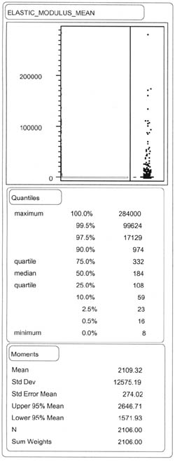
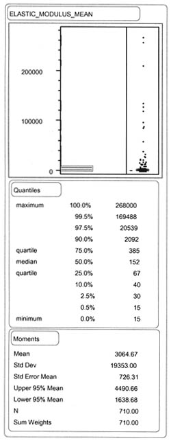
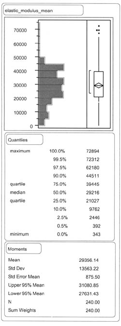
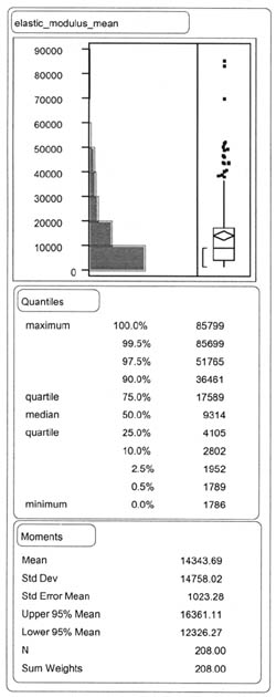
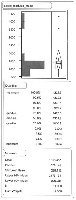
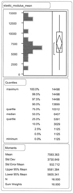
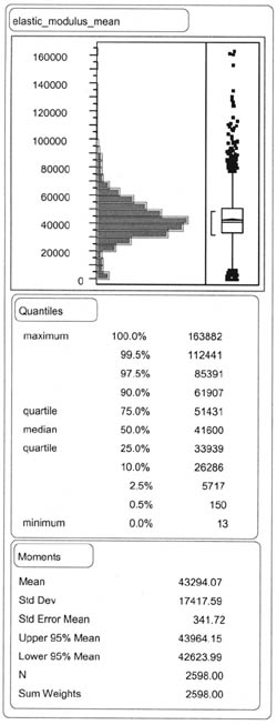
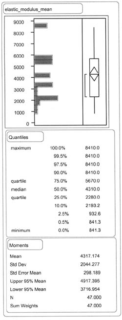
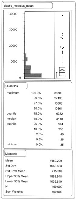
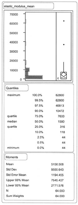
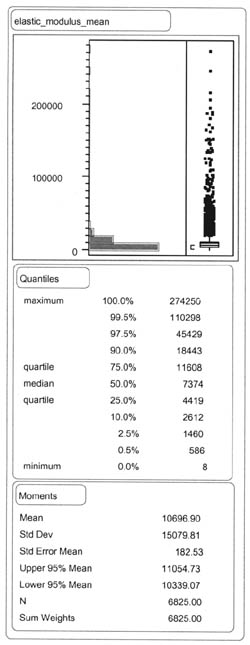
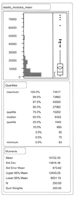
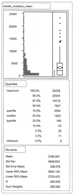
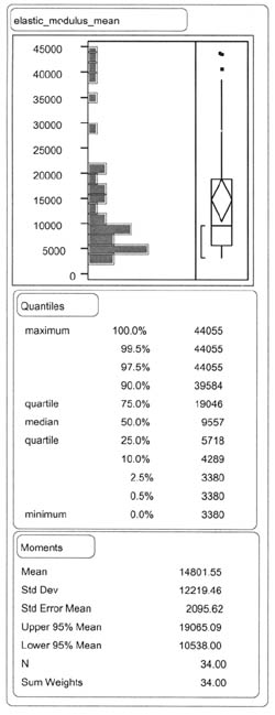
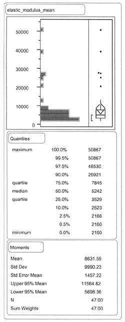
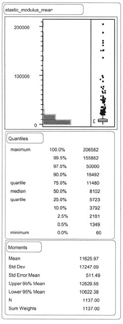
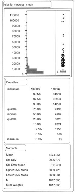
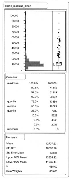
Histograms of Back-Calculated Young's Modulus of Flexible Pavements for Subgrade Soils Separated by the AASHTO Soil Classification System:
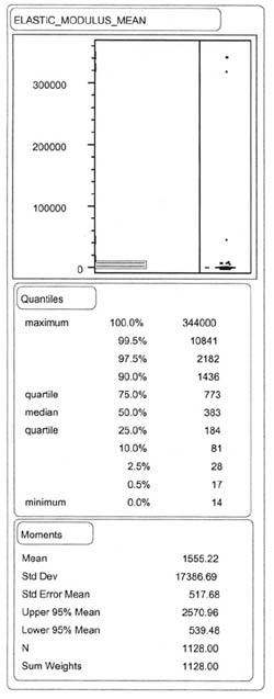

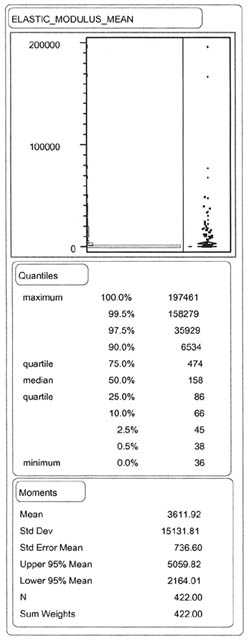
Histograms of Unbound Aggregate Base and Subbase Layers for Flexible Pavements


 D
D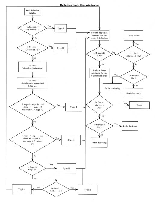 D
D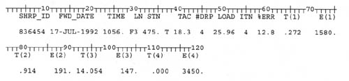 D
D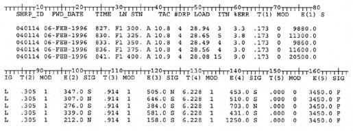 D
D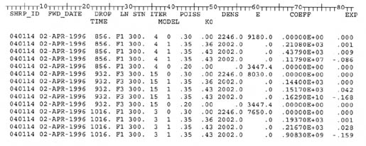 D
D