U.S. Department of Transportation
Federal Highway Administration
1200 New Jersey Avenue, SE
Washington, DC 20590
202-366-4000
Federal Highway Administration Research and Technology
Coordinating, Developing, and Delivering Highway Transportation Innovations
 |
| This report is an archived publication and may contain dated technical, contact, and link information |
|
Publication Number: FHWA-HRT-10-038
Date: October 2010 |
||||||||||||||||||||||||||||||||||||||||||||||||||||||||||||||||||||||||||||||||||||||||||||||||||||||||||||||||||||||||||||||||||||||||||||||||||||||||||||||||||||||||||||||||||||||||||||||||||||||||||||||||||||||||||||||||||||||||||||||||||||
Balancing Safety and Capacity in an Adaptive Signal Control System — Phase 16.0 PHASE 2 RESEARCH AND DEVELOPMENT6.1 OBJECTIVES FOR PHASE 2 RESEARCHThe objective of the second phase of this research is to develop a methodology to balance efficiency of traffic flow and traffic safety in the operation of adaptive traffic signal systems on arterials and grids. In phase 1, the relationships between traffic signal timing parameters and safety performance were explored. Fifteen test cases were constructed to identify isolated correlation effects between changes to one signal timing parameter and a relative change in safety performance. Safety performance in phase 1 was estimated using the FHWA SSAM tool and the VISSIM® traffic microsimulation model. Analysis results in phase 1 indicated that there are measurable and statistically significant differences in the generation of conflict events when modifying several of the signal timing parameters in the test cases. At the same time, changes to the signal timing parameters have appreciable and measurable effects on efficiency of traffic flow as reflected in performance measures such as stops and delay. The next step in the research is to develop a methodology and algorithms for balancing improvements in efficiency and safety that can be used to adjust signal controller timing parameters in a real-time adaptive manner. This section outlines the plan for the methodology and algorithm development in phase 2 of the research project. The first step of the methodology is to develop a multiattribute safety performance function. The safety performance function is used to predict and evaluate the relative changes to safety performance when modifying any or all of the traffic signal controller parameters that are considered as inputs. This function would then be used in conjunction with a performance function for traffic efficiency to balance the effects of safety and efficiency when making changes to the signal timing parameters. The first part of this section details the process for developing the multiattribute safety performance function. Subsequent parts describe how the safety performance function and traffic efficiency function can be combined to balance efficiency and safety in a real-time adaptive manner. 6.1.1 Extending the Conflict Analysis Approach to the Next Phase of Research In this project, a methodology is being developed to balance safety with efficiency in changing signal timing parameters. Whether these parameters are adjusted in real time or infrequently, the first task is to establish the relationships between the signal timing parameters and the change in safety performance. Similarly, a separate performance function for the change in the efficiency (stops and delay) based on the change to the signal timing parameters must be established. In either online or offline signal timing optimization, a traffic performance model is used to predict the performance of various signal settings. A performance model indicates that the efficiency of a given set of input parameters is X', where the current performance of the unchanged parameters is X. If X' is better than X, this direction of change is considered positive and further exploration of changes in that direction are considered. A search method is used to explore all possible, or all reasonable, signal settings until no significant performance improvement can be obtained by further tweaking the parameter values. Different search methods must be selected based on the format of the performance functions. For example, if the functions are all linear equations, very fast and efficient algorithms are readily available. Nonlinear equations require more sophisticated mathematical techniques. Simulations require iterative approaches that are typically time consuming. In any case, the next step is to identify the format of the safety performance function to be used in phase 2 of this research. The preliminary analysis done with SSAM has established that certain parameters have positive correlations with changes in safety, but this analysis cannot be used directly to determine the magnitude of effects. In addition, each parameter has been evaluated in isolation. In a real-world, real-time setting, changes to these parameters must be evaluated simultaneously and in an integrated fashion. There are primarily two ways to accomplish the incorporation of a safety performance function in the selection of signal timing parameters:
Either option presents a multiobjective optimization problem in which the goal is to identify signal timing settings that either are beneficial for both efficiency and safety or provide a trade off between improving one or the other according to some preference determination. 6.1.2 Choice of a Safety Performance Function As identified above, there are two primary choices for establishing a performance function engine for the multiobjective optimization problem. Simulation in-the-loop optimization analysis, using SSAM and a microscopic simulation tool such as VISSIM® in the loop with the optimization search methodology, is a high-fidelity approach. In this approach, SSAM would be used as an exact performance assessment tool that can be used to directly evaluate the changes to conflict rates when modifying one or more traffic signal timing parameters. This approach is very time consuming and has little chance of transferring to online, real-time operation due to the following obstacles:
The second, and preferred, methodology to establish a safety performance function is to develop a regression-equation relationship between signal timing parameters and safety performance. Such an approach is executable for both offline and online operation. This approach is similar to traditional crash prediction, except that the prediction domain is sufficiently higher fidelity than predicting the crashes that might occur over the next year. Using a regression-equation approach, the safety performance function would evaluate how the conflict occurrence rates would be perturbed over, for example, the next 15 min at the same input traffic demands. In this approach, the following function is established:(18,19) The safety performance index might be defined as the total number of conflicts at the intersection or as some combination of the different types of conflicts. This functional relationship is likely to require nonlinear terms and interactions between the inputs rather than simply a linear combination of the various input parameters. For example, one will likely need to compute a derived measure of traffic demand or degree of saturation for each phase, rather than directly input the traffic volumes. Before further discussing the methodology for developing the safety performance function, the type of adaptive operation to be developed in phase 2 must be identified. 6.1.3 Candidate Adaptive Control Signal Timing Optimization Strategies As identified above, there are two primary choices for establishing a performance function engine for the multiobjective optimization problem. Simulation in-the-loop optimization analysis, using SSAM and a microscopic simulation tool such as VISSIM® in the loop with the optimization search methodology, is a high-fidelity approach. In this approach, SSAM would be used as an exact performance assessment tool that can be used to directly evaluate the changes to conflict rates when modifying one or more traffic signal timing parameters. This approach is very time consuming and has little chance of transferring to online, real-time operation due to the following obstacles: The following are the three primary strategies employed by all adaptive control systems currently in use across the world:
For this project, only the second two methods are considered viable. The authors believe that real-time, second-by-second control of signal timing for evaluation of safety would only be possible with IntelliDriveSM technologies or simple if/then type approaches such as those employed by Zimmerman and Bonneson's DCS system to extend red or yellow clearances due to imminent crash situations.(1) Based on past experience with both RHODES and ACS Lite, it is presumed that real-time safety analysis could not be reliable enough or processed quickly enough to be integrated with a traffic efficiency calculation methodology such as that employed by RHODES or OPAC. Pattern matching is an approach that has been used in traffic control systems since the development of the minicomputer and the urban traffic control system over 35 years ago. This approach requires a sophisticated user to develop signatures and rules and requires extensive setup and testing. Most traffic responsive modules of ATMS systems are not used to their full potential due to the difficulty in determining what the signatures or thresholds should be, the lack of reliable input data (i.e., volumes) to drive the decision-making algorithms, and the effects of frequent signal controller transition (i.e., offset and cycle seeking) on traffic performance. A parameter-tuning approach is much more reasonable than either of these two alternatives based on the experience of the researchers in the FHWA ACS Lite development project.(20) Parameter tuning allows the local signal controller to continue to operate the intersection on a second-by-second basis while the external processor handles the more complex decision making to make small adjustments to the signal timing parameters to improve safety, efficiency, or both. A parameter-tuning approach avoids many pitfalls of traffic-responsive methods since it embeds much of the "intelligence" in the algorithms and thus requires less user setup. In addition, drastic transitions from one cycle/offset combination to another are avoided by limiting the parameter changes to only small adjustments from the current settings. Since a parameter-tuning approach only runs its optimization algorithms at minimum once every three or four cycles, the additional processing burden to evaluate safety performance and perform the trade-off analysis to balance efficiency and safety can probably be accommodated in the processing time available. The general methodology for the adaptive control algorithm that balances safety and efficiency will be as follows:
6.1.4 Candidate Signal Timing Parameters that Affect Efficiency and Safety Phase 2 will develop a traffic-adaptive strategy that tunes the following parameters to improve safety, efficiency, or both:
These parameters will be tuned every 5–15 min based on phase-timing data and detector data obtained from the signal controller. Similarly, these parameters are frequently tuned in an offline manner in tools such as TRANSYT and Synchro™. In addition to these tuned parameters, the adaptive control system will evaluate delaying or accelerating the change from one time-of-day (TOD) pattern to the next based on the perceived benefits to safety and efficiency. Experience operating traffic signal control systems and designing signal timing plans for grid and arterial systems has shown that these parameters all have an appreciable effect on efficiency. Performance measures and algorithms for tuning these parameters have been developed in the past, for example, in the FHWA ACS Lite project.(20) These measures will be presented in a later section, where the algorithm is described in more detail. The initial analysis using the SSAM tool in this research project also indicated that these parameters have an effect on the safety of an intersection, as represented by appreciable and statistically significant changes to the total conflicts that occur when the parameters were changed. Each of these effects on safety was tested and evaluated separately, so the next step will be to test and evaluate their effects in combinations. This is a necessary step in the development of the safety performance regression functions that will be used to predict the effects of changes to the parameters in the adaptive control algorithm. 6.2. EXPERIMENTAL DESIGN6.2.1 Design of Experiments for Identifying Safety Regression Parameters As identified previously in this research, the aforementioned input parameters (cycle time, phase sequence, etc.) were found to have individual effects on the safety performance of the signal system in the limited tests that were conducted. These data are not sufficient to identify a generalized prediction of the effect of changing these parameters, evaluated individually or in combinations. For example, one test showed that conflicts increased 25 percent when the cycle time was changed from 70 to 100 s. This result says little about the change in conflicts when the cycle time is changed from 100 to 130 s and at different traffic volumes. In the limited testing that was performed, nonlinear effects were observed in almost all of the parameters evaluated. So, the rate of change or gradient of conflict is not constant, and thus, a functional relationship must be calibrated. In statistical regression modeling, this combinatorial problem can be addressed by using a designed experiment. A designed experiment attempts to maximize the information gained on each run of the experiment by combining the input factors in special ways so that both the boundaries and the center of the design space are covered by evaluation runs and by performing a minimum number of runs without having to evaluate all possible combinations of the inputs. In the present problem, consider the following representative options for each input parameter for a typical eight-phase dual quad intersection with left-turn phases in all directions:
This yields 3 × 4 × 6,561 × 16 × 81 = 102,036,672 combinations without including variations in the approach demand volumes. Clearly, this many simulation scenarios do not need to be evaluated to obtain enough information to fit the regression models to the data. Symmetry in the input-parameter structure can be used to reduce the replicates immensely, particularly in the evaluation of the combinations of the split settings. For example, the difference between phase 1 and phase 5 having a certain level of saturation (all other inputs being equal) is the geometric location of the phase at the intersection. To an evaluation algorithm, the situational data appear identical, and—all things such as turning-bay lengths being equal—one would expect the recommended changes to the parameters out of an optimization algorithm to look the same as well. 6.2.2 Design of Experiments to Reduce the Number of Runs There are many approaches to design of experiments that could be applied. The most common approach for linear regression models is a 2k fractional factorial design. There are several variations of this approach, but in general, a fractional factorial design is used when single factors are hypothesized to have linear relationships with the output measure. There may be interactive effects between input variables, but no quadratic or other nonlinear terms are assumed to be included for an individual input in the underlying model form. This is not likely the case in the present situation, but more detail on the fractional factorial process is provided for the purpose of explanation. A fractional factorial designed experiment uses one of two levels of each input variable in each replicate run. Then, a smaller number than the total full factorial matrix of combinations is actually run, such as 2k-3 or 2k-5. This smaller number of replicates is based on assumptions about the lack of significance of higher-order combinatorial effects in the resultant model. A typical model format for 2k-n fractional designs is: In this model, all effects of the input parameters are either linear or cross-product terms of two of the inputs. The current design problem does not exactly match this format since engineering judgment indicates a need for more than two settings for each input parameter to fit an appropriate model. The runs are then expressed as a matrix of +1 and -1 indicator variables where +1 indicates the high value of a variable and -1 indicates the low value of a variable. For example, in this problem, a high value of a cycle time might be 150 s and a low value would be 60 s. Since the relationships between inputs and outputs are individually assumed to be linear functions in this type of model, it is not necessary to obtain data at 120 s, 90 s, etc. since these outputs can be estimated from the regression equation. The pattern of combinations used in this approach is shown in table 40. Table 40. Fractional factorial design approach using linear regression models.
Clever determination of the combination of +1 and -1 factors of all of the input variables allows maximum information to be gained from just a few iterations of the design space if higher-order interaction terms can be assumed to have negligible impact on the performance of the regression relationship. The use of dummy variables +1 and -1 avoids difficulties with the matrix inverse computations (necessary to solve for the regression coefficients) that arise when input variables have vastly different scales. However, that is not the case in this particular application since all of the potential input parameters are in seconds or can be encoded as integer values. For example, the variable for protected/permitted left turn could be coded as 3 for permitted only, 2 for protected/permitted, and 1 for protected only. To obtain meaningful regression coefficients, it is important to choose the coded values appropriately based on what one would expect to happen to the output variable when the coded value is changed. In this example, the highest value of the code being associated with permitted-only left turns would match earlier results that indicated that conflicts are more plentiful in this situation than in the other two situations. This is the basic concept of design of experiments: identify the meaningful input variables and potential interaction effects, and identify a matrix of combinations that provides enough data to solve for a set of regression coefficients. Goodness of fit is then typically tested by comparing the model against real results (in this case, the number of conflicts per hour) for a few situations that were not used in developing the model parameters. Engineering judgment indicates that the relationship between the input parameters and the conflict (safety index) output is nonlinear. Although other forms can be chosen, a typical nonlinear regression equation is expressed as: In the design of experiments literature, a more appropriate design for a nonlinear regression model is called the central composite design (CCD). This type of design allows the assessment of the curvature of the nonlinear terms by using five potential settings for the input parameters (+sqrt(2), +1, 0, -1, -sqrt(2)). A slightly larger number of runs results from use of CCD instead of fractional factorial design, but the combination of variable settings follows similar patterns, as can be seen in table 41. Table 41. CCD approach using nonlinear regression models.
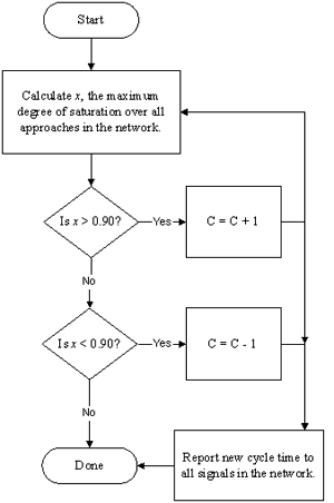
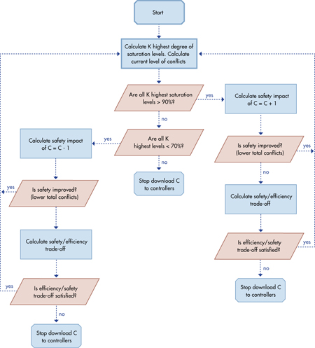
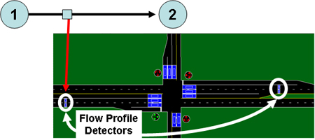
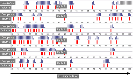
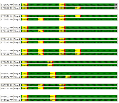
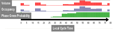
These values are chosen to maximize the statistical properties of the design of experiments process for quadratic equation. In the actual application, a similar process will be used to choose the run combinations and settings based on the single-variable relationships. After the experimental runs are determined, three VISSIM®/SSAM runs will be performed at each combination of settings, and the average total conflicts and the average of each type of conflict will be obtained. Based on the number of combinations that must be performed, no more than three iterations are sustainable within budgetary and schedule constraints. It is also likely that a single run at each combination could suffice. The regression coefficients can then be obtained from a statistical analysis package such as SPSS®, SAS®, or Microsoft Excel®. Another smaller set of input combinations is then typically used to test the goodness-of-fit of the resulting model by comparing the actual output from the simulation model with the prediction from the regression equation. These input combinations are not typically used in the development of the regression model. This functional—total conflicts or a cost-impact weighted combination of the conflict types—would then be used as the safety performance function in the search process that trades off or finds the balance between efficiency and safety for each of the control parameters (cycle time, splits, offsets, phase sequence, and protected/permitted left-turn settings) in determining the new signal settings at each iteration. 6.2.3 Multiobjective Optimization Approach The parameter-tuning approach for adaptive control is a middle ground between fully adaptive, second-by-second control of traffic signals and rule-based traffic-responsive systems. Fully adaptive real-time control systems require sophisticated simulation modeling to evaluate the effects of changes to the parameters on the performance criteria. For example, in RHODES, queues in each lane at each approach are modeled and traffic is tracked from upstream locations on a second-by-second basis. A dynamic programming algorithm is used to evaluate the resultant traffic delay based on assessment of several options for what the signal timing settings might be in the next 60 s or so. The signal timings that result in minimum delay are selected for implementation. A few seconds later, the entire process is repeated in a rolling-horizon fashion. RHODES is very sensitive to accurate determination of the queues and requires a multitude of parameters for queue discharge speeds and the like that must be calibrated to field conditions. Past experience leads to the belief that another RHODES- or OPAC-like algorithm is inappropriate for development until data from IntelliDriveSM systems are readily available. On the other hand, a traffic-responsive system can have relatively simple if/then rules that identify when to switch from one traffic-control strategy to another. In predictable situations, this type of operation can be very effective, such as when a certain demand level is tripled or quadrupled very quickly (for example, when a special event is concluded). In generalized situations, however, traffic-responsive systems become onerous to configure, requiring the consideration of every possible situation and the embedding of that information into the system of if/then rules or detector data signatures that are used to match the field conditions with the desired control strategy. The parameter-turning approach strikes a middle ground by allowing more robust solution of the signal timing settings than traffic-responsive operation but with more predictable behaviors than real-time systems because it starts from a given set of TOD pattern parameters and only tweaks those settings incrementally over time. These tweaks adjust the signal timing operations to react to the statistical fluctuations of traffic flows, correct any errors that have been made in determining the initial settings, and react to special events, incidents, and short-term changes to traffic flow patterns. By operating within a given set of boundaries, such as not changing the signal timings too dramatically from their initial values, the parameter-tuning approach is safer and more reliable than real-time approaches that override the signal controller. In addition, since a parameter-tuning system is not predicated on running a detailed traffic model to evaluate performance, it has fewer challenges with calibration and is less reliant on perfect detection accuracy. As was done with ACS Lite, this project will develop algorithms that select new signal timing settings from simple models of changes to traffic efficiency and the regression-model approach for estimating the changes to safety. For this situation, there is not likely to be a single solution that simultaneously optimizes both objectives. In this case, the goal is a solution in which each objective has been optimized to the extent that if optimized any further, the other objective will suffer as a result. Finding such a solution and quantifying how much better it is compared to other such solutions—and there will generally be many other feasible options—is the goal when setting up and solving a multiobjective optimization problem. 6.3 Five Principle Algorithms of the Adaptive Control Approach to Balance Safety and EfficiencyThis section discusses the five principle algorithms included in the proposed adaptive system operation. Cycle time is most often selected on a section- or arterial-wide basis to facilitate progression and to provide adequate capacity to operate all of the signals in the subsystem under capacity. Most often, cycle times in adaptive control systems are chosen according to a heuristic rule, or in the case of real-time, second-by-second systems, the concept of cycle time is transient—the cycle length can change in each iteration as the system operates more like "free" intersections than in coordination. For example, SCATS® uses a heuristic that might be termed the "90 percent rule." The SCATS® cycle for a section is ratcheted up or down based on keeping the most saturated intersection in the section at a 90 percent degree of saturation. This is a reasonable strategy to follow and guarantees that the cycle selected will not artificially cause congestion in certain approaches. In a simplistic fashion, if the cycle time is increased by X seconds, then every phase on the controller gets a proportion of the additional time. For example, if 4 s are added to the cycle time and there are four phases per ring, one additional second is provided for each phase split. A simple approach for tuning cycle times is depicted in Figure 23. This strategy will tend towards longer cycles during peak periods as traffic demand builds, which is appropriate despite recent research indicating that when the conditions are extremely oversaturated, shorter cycles will provide more efficient throughput. At this point in this research project, the case of extreme oversaturation is ignored and the multiobjective adaptive system is designed for normal operating modes. The research team can return to the consideration of oversaturated conditions after the baseline system is developed and proven effective. Figure 23. Chart. Generic cycle time tuning algorithm to keep all intersections below 90 percent degree of saturation. This approach is too simplistic, however, for the following reasons: (1) the consideration of the safety performance of the candidate cycle time must be included, (2) the interaction between the recalculation of the splits must be taken into account before selecting a new cycle setting, and (3) allowing the maximum degree of saturation to be taken from all phases in the system also tends to overreact to minor movements that are at their capacity. A small improvement to this heuristic is to consider some k highest saturation levels—or some determination of critical approaches or movements—throughout the network and only increase the cycle time when a minimum number of those critical links are above the 90 percent level. Similarly, decreasing the system cycle when all approaches are less than 90 percent may not be desirable to maintain adequate progression. To combine the effects of both safety and efficiency, evaluation of the safety performance function is included in the algorithm for adjusting the cycle time as shown in Figure 24. Figure 24. Chart. Flow chart of cycle time tuning algorithm. In this manner, the possible improvements to both safety and efficiency are considered by first checking the efficiency metric for the cycle time. It must be determined if all of the k highest saturation levels are above or below 90 percent. If there are at least k movements with saturation levels above 90 percent, an increase to the cycle time is considered. If this change results in improvement to the safety metric, reducing the total predicted conflicts, this direction is followed until it begins to degrade safety performance or when one or more of the k highest saturation levels has fallen below 90 percent saturation (or whatever threshold is determined to be appropriate). When the safety performance does not continue to reduce the total number of conflicts, a safety efficiency trade-off metric is computed. Based on the current preferences, it is determined whether to continue to increase the cycle time at the expense of safety. If so, it is increased until the metric falls below the threshold, and then it is stopped. Similarly, in the opposite direction, reducing the cycle time is considered if there are more than k' (where it could be true that k is not the same as k', but there is currently no judgment to determine that this is the case) movements with saturation level below 70 percent (or whatever threshold is determined to be appropriate). If this is true, a reduction to the cycle time is considered and the system cycle time is reduced until the safety trade-off metric is violated or there are no longer k' movements with saturation level below 70 percent. Cycle time tuning affects all of the intersections in the network if they are all operating in a coordinated mode. Individual intersections that are run "free" can also have their cycle time tuned independently. Tuning offsets improves progression performance along primary routes for phases that are coordinated. Offset tuning algorithms are particularly straightforward. The methodology used in the ACS Lite project will be used in this project.(20) The concept of the data-driven offset adjustment algorithm is summarized in two simple statements: (1) use detectors several hundred feet upstream of the signal to construct cycle-based profiles of traffic flow arriving to the intersection, and (2) adjust the offset to maximize the number of vehicles arriving during the green phase. This simple concept is then expanded to consider and mitigate the effects of such modifications to the offset value for two-way traffic and the effects of changes at this intersection on adjacent intersections. Periodically, small, incremental adjustments are made to the offset to maximize the total proportion of cyclic flow arriving to a green light. It is assumed that an initial solution (plan data—cycle, splits, and offset) has already been developed and that the original offset may be less than optimal. A user-configurable maximum deviation from the original setting—either an increase or decrease to the offset value—is defined for each offset to restrict the algorithm from drifting too far away from the original solution. Figure 25 illustrates the detector locations used for offset tuning. There is one detector station for each coordinated approach. Intersection 1 is referred to as the upstream intersection, and intersection 2 is referred to as the downstream intersection. Traffic volume and occupancy are measured at some point between 1 and 2 by a detector in each lane. These detectors can be located where typical advance detectors are located, 200–300 ft from the intersection. Placing detectors further upstream can improve the quality of the flow rate measurements and reduces the possibility of vehicles queuing over the detectors when the light is red. It is also not necessary to have one detector per lane returned to the controller in a separate amplifier, but this practice will improve performance of the algorithm. Figure 25. Illustration. Typical flow profile detector locations on coordinated approaches. Assuming that the traffic signals at both intersections are using the same cycle length and that traffic volumes and turning proportions are reasonably steady over time, it is expected that the detector will measure approximately similar recurring patterns of flow during each cycle. These patterns of flow are referred to as cyclic flow profiles or just flow profiles. Figure 26 plots the flow profile data (volume and occupancy observations) as a function of the local cycle time of the controller (time is on the x-axis). The magnitude of the volume and occupancy is indicated by the height of the corresponding bars in each row of the chart. The height of the bars in each row is scaled by the maximum value observed in that row. Equal heights in different rows do not necessarily indicate the same volume or occupancy value. These profiles indicate that it is typical over the last few cycles for traffic to arrive near the beginning of the local cycle time for this approach. Secondary platoons and individual vehicles also show up randomly throughout the cycle, possibly due to turning flow on the cross-street phases of intersection 1 and/or early return to green due to side-street gap-outs. Figure 26. Illustration. Example of volume and occupancy data from a typical advance detector. Figure 27 illustrates an example of phase timing history observed over the last several cycles at an intersection (note that the data from Figure 26 and Figure 27 are not from the same location). Figure 27. Illustration. Example of phase timing for each of the last several cycles. The number and color of each column in the timeline corresponds to the active phase interval (green, yellow, and red) displayed by each ring at that time in the cycle. All subsequent cycles shown below the first row are actual data recorded from a field test controller with the most recent data at the top and progressing back in time down the display. Each cycle begins at the local zero time, which is labeled on the left. Note that the duration of non-sync, actuated phases (typically phases other than 2 and 6) are variable, and one or more of these phases may be skipped in any given cycle. Thus, the time at which the controller returns to the sync phases (typically phases 2 and 6) can and does vary from cycle to cycle. The cyclic flow profiles illustrated in Figure 26 are then averaged to generate a single, representative cyclic flow profile for the flow profile detector as shown in Figure 27. Each link, and thus each flow profile detector on that link, is associated (via user configuration) with a corresponding phase at the downstream intersection, referred to as the progression phase. Figure 28 shows a single cyclic representation of the percent of time that the progression phase was green during the several cycles since the last offset adjustment control decision. The height of the green bar in the display denotes a range of 0–100 percent. Note that in the case of an arterial, the progression phases generally correspond to the coordinated phases on the controller. In a grid network, all major through phases (coordinated and non-coordinated) might be configured as progression phases for their corresponding approaches. Figure 28 shows that during a portion of the cycle, the progression phase is green 100 percent of the time, starting at local time 50 and ending at local cycle time 0 (or 80). During each cycle, one or more non-sync phases typically gaps out early, and in such cases, the controller returns to the coordinated phase earlier than is required, typically termed "early return to green." Figure 28 illustrates this early return to green behavior with the tapering percent-green bars prior to the programmed start of main street green split (local time 50 s). As shown, this progression phase started as early as local cycle time 27 in at least one cycle during the last ~10 cycles. Figure 28. Illustration. Example of cyclic volume and occupancy profiles averaged over the last several cycles. Figure 28 also displays the detector data from the flow profile detector shifted to account for the unimpeded travel time from the upstream detector location to the theoretical "green point," where a driver would likely decide to stop if the light were yellow and continue if the light were green. This time is configurable by the user based on input of an average travel speed and distance from the detector to the stop line. Detectors that are thus located at the theoretical decision point are not shifted at all, and in cases where the detector is placed closer to the signal than the green point, this shift may be negative. Note that occupancy, rather than volume, is currently the preferred detector measurement used to generate flow profiles. Thus, the term flow profile is used to refer to shifted occupancy cyclic flow measurements rather than volume. The flow profile scenario shown in Figure 28 is an example of the performance of a good offset for one-directional travel. The arriving platoons are indicated by the cluster of relatively tall occupancy bars between local cycle time 40 and local cycle time 75, which corresponds to the green portion of the service phase. 6.3.2.1 Captured Flow The effectiveness of two offset settings or the relative difference between the two settings at upstream and downstream intersections is quantified by calculating the progressed flow or captured flow. This performance measure is a surrogate for stops and delay, which cannot be directly measured in the field from point detectors. Specifically, the captured or progressed flow is the amount of flow (in units of vehicle-seconds of occupancy) arriving to the stop line at a given point in the cycle multiplied by the percent of time the progression phase is green at that time during the cycle. The algorithm evaluates different offsets by calculating the captured flow on each approach and selecting the offset that maximizes the total amount of captured flow. 6.3.2.2 Distributed Offset Adjustment The methodology that will be used is a distributed offset adjustment method. This approach makes offset adjustments for each controller independently with consideration of the effects of each independent decision on adjacent signals. Each controller considers three offset settings: no change, adjust to 6.3.2.3 Including Safety in the Assessment of Offset Performance The approach to tuning offsets previously discussed will be modified to include the evaluation of the safety impact of the adjustment. Similar to the approach for tuning the cycle time, the algorithm will use the safety performance regression equation as the performance calculator. This approach is detailed in the flow chart in figure 29. An enhancement to the methodology used by ACS Lite will also be applied. This adjustment will allow continuous evaluation of offset adjustment options (i.e. ±1 second, ±2 seconds, ±3 seconds, …±10 seconds, etc.) instead of considering only three options for offset adjustments (i.e +2 seconds, -2 seconds, or zero). As identified by Gettman et al. this extension to the approach will provide more rapid response to offsets that are performing particularly poorly.(20) Figure 29. Chart. Offset adjustment algorithm flow chart. As shown in figure 29, the general approach is to identify the capture efficiency performance of options to move the offset forward or backward. If one or the other improves performance over the "no change" situation (note that it is not common or probable that both moves improve performance), the safety impact of the proposed change is checked. If this change is deemed to improve both safety and efficiency, the algorithm will continue exploring this direction of change for additional improvements. If the change is deleterious to safety, the algorithm checks if the trade-off value is satisfied, asking if the effect on safety is not significant enough to disallow exploration in this direction. The algorithm continues until the effect on safety is deleterious or no longer improves the capture efficiency. The approach used to tune splits is driven by collecting the same data used to tune offsets—phase timing information and second-by-second detector occupancy and volume—but the data are collected from detectors at the stop bar of the intersection. This methodology is also derived from the algorithms developed in the ACS Lite project. In general, this approach to tuning split times is derived from the concept used by SCATS® and SCOOT, which is to equalize the degree of saturation on all the phases at the intersection. In shorthand, this approach is termed "equisat." To be specific, the algorithm in ACS Lite minimizes the maximum degree of saturation on any phase rather than driving all of the saturation levels to the same value. This algorithm also allows coordinated phases to have biased splits, so that progression is protected when the saturation level of the coordinated phase is lower than that of side streets. Without such biasing, the performance is slanted toward providing adequate levels of service on side streets, which neglects the throughput issues. The approach works by balancing a measure of degree of saturation that is termed "phase utilization." 6.3.3.1 Split Constraints There are constraints on split adjustments which can be defined using a phase-barrier diagram. A typical phase-barrier sequence is illustrated, with barriers explicitly labeled, in figure 30. Figure 30. Diagram. Ring diagram with barriers denoted by bold vertical lines. In discussing the split adjustment algorithms, it is necessary to refer to certain groups of phases. The collection of phases on a particular ring, between two particular barriers, is referred to as a ring group. In figure 30, there are four ring groups: (1, 2), (3, 4), (5, 6), and (7, 8). A barrier group is the collection of all phases (or all ring groups) between two particular barriers. In figure 30, there are two barrier groups: (1, 2, 5, 6) and (3, 4, 7, 8). The algorithm uses these groups to swap split time from one phase to another in order to determine the set of split adjustments that satisfy the cycle time. It is necessary to determine the legal range of adjustments for each split before solving for the set of split values recommended for a given controller. This includes consideration of minimum times, maximum times, and pedestrian crossing restrictions. These constraints are also important to calculate for each ring and barrier group. While this may seem trivial, it is important to accurately calculate these values before searching the optimization space as consideration of these limits significantly improves the calculation efficiency. 6.3.3.2 Calculation of Duration Constraints The following algorithm identifies the necessary steps for calculation of the constraints to be considered when searching for the optimum splits at each intersection. 1. Compute the minimum, current, and (initial) maximum split durations for each phase p,
2. Compute the minimum, current, and (initial) maximum durations for each group g.
3. Calculate the revised maximum duration for each barrier group, its corresponding ring groups, and the maximum phase splits of their corresponding phases.
6.3.3.3 Estimating Phase Utilization The split adjustment algorithm that will be used in phase 2 is based on the notion of balancing the utilization of all phases of a signal controller. Prior to discussing the algorithm itself, it is necessary to define the following:
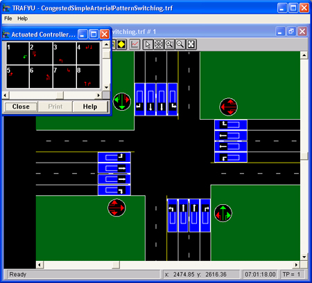
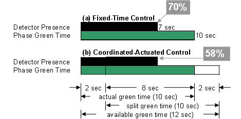
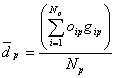
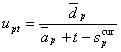
Phase utilization is the effectively utilized percentage of available split time. It is analogous to the degree of saturation concept, which is also referred to as the V/C ratio. Utilization is used instead of degree of saturation since the degree of saturation is calculated using volume and capacity counts or rates. Utilization is calculated using ratios of used green time to available green time. The used green time comes from occupancy of the detector. Figure 31 illustrates a typical detector layout for measuring phase utilization with a detector placed at the stop bar for each lane. Each detector is associated with the phase that serves traffic flowing through its corresponding lane. Detector dimensions do not have to be the theoretical "best possible length." Figure 31. Screenshot. A complete utilization-detector layout for ACS Lite. The methodology measures the demand for a phase by monitoring the occupancy of the phase during green. Demand is measured in terms of time, rather than volume. Utilization is given by the ratio of demand time to available green time. This is illustrated in figure 32. Figure 32. Illustration. Measuring phase utilization for coordinated-actuated controllers. The system to be developed in phase 2 will poll controllers for phase timing and detector data once per minute and aggregate the data over time, combining several consecutive once-a-minute poll responses to construct estimates of occupancy during green, green phase duration, and utilization. Figure 32 illustrates an example where 10 s of green is served, during 7 s of which the detector is occupied. For a fixed-time controller, this corresponds to 70 percent utilization. However, in the context of a coordinated, actuated controller, the capacity of the phase is measured as the amount of available green time. In this case, the phase started timing green 2 s early due to a prior phase gapping out early. It could serve up to 12 s of green until it is forced off, but it gaps out after 10 s of green. The notion of available green includes the remaining time to the force-off or maximum green, whichever comes first. It is also important to consider when phases have been skipped due to lack of demand. Similar to the offset adjustment algorithm, the splits will not be tuned without collection of at least three recent observations of each phase while the controller is in coordination (i.e., when the controller is in transition or preemption, the algorithm will not use these data in tuning splits). Having satisfied this condition, the algorithm then calculates the utilization of alternate split durations for each phase using the following variables and equations, where: Np = Number of observations of phase p. oip = Occupancy of phase p green time during observation i (0–100 percent). gip = Green time served by phase p during observation i (seconds). aip = Available green time for phase p during observation i (seconds). dp = Average demand (seconds occupied green) per cycle for phase p. ap = Average available green time (seconds) per cycle for phase p. cp = Clearance time (seconds of yellow and all-red) associated with phase p. upt = Utilization estimate for phase p with split of duration t seconds. 6.3.3.4 Estimation of Split Utilization The calculation of the split utilization is the primary prediction of how well or how poorly an alternative split allocation will perform when implemented. This prediction model is rather simplistic, but it presents a reasonable approximation when traffic is not rapidly increasing or rapidly decreasing in demand. The mathematical process to determine this function is as follows: 1. If Np < 3, then stop—there is not enough data for split adjustment. 2. Compute average demand, 3. Compute average available green time, 4. For each feasible split duration t, between
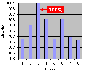
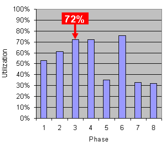
After calculating the estimated utilization levels for all alternate split durations, an iterative algorithm is executed to select the combination of split values that satisfies the constraints on each phase and phase group (i.e., ring and barrier groups) and minimizes the maximum utilization of any phase on the controller. This procedure is discussed in the next section. 6.3.3.5 Balancing Utilization Levels Each phase is assigned a utilization measure that approximates the degree of saturation of that phase, which ranges from 0 to 100 percent or higher, if oversaturated. Utilization is estimated for each phase for the full range of possible split durations, as discussed in preceding sections. Figure 33 is an example of utilization estimates for a dual-ring, eight-phase controller where the utilization of phase 3 is very high. Figure 34 is a chart of the estimated utilization of phases after the algorithm has adjusted the splits to minimize the maximum utilization of any phase on the controller. Figure 33. Graph. Utilization of phases before split adjustment. Figure 34. Graph. Utilization of phases after split adjustment. The changes in split times are listed in table 42. The bold text in table 42 highlights the change of the most utilized phase from 100 percent to 72 percent. Also note that the new maximum phase utilization is now on phase 6, which has increased from 72 percent utilization to an estimated 76 percent utilization. Note that the result of the adjustment is not the exact same utilization level on each phase. Table 42. Example utilization of phases before and after split adjustment.
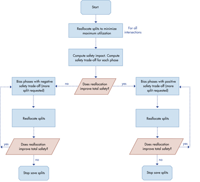
As indicated previously, the primary objective of the split adjustment algorithm is to minimize the maximum degree of utilization across all phases. These objectives achieve the general effect of balancing the degree of utilization across phases. Webster suggested as early as 1958 that allocation of splits to equalize the degree of utilization across all phases will have the effect of minimizing delay.(21) In the ACS Lite project, it was found that less than a dozen iterations of the balancing algorithm will typically result in a reallocation that minimizes the maximum phase utilization of the intersection. This does not consume an appreciable amount of CPU time, and thus, the addition of safety analysis should not impact the ability of the system to complete processing in a reasonable time frame. 6.3.3.6 Incorporating Safety Assessment in the Optimization of Splits Similar to the approach used for cycle time and offset tuning, the algorithm for splits will incorporate evaluation of safety into the optimization by utilizing the safety performance functions developed at the beginning of phase 2. This process is illustrated in the flow chart in figure 35. First, the reallocation algorithm is run to identify the set of splits that optimizes only efficiency. This set of splits is then input into the safety performance function and evaluated. The safety/efficiency trade-off is also calculated for each split. If the reallocated splits improve total safety, then the splits that have positive safety trade-off are identified for biasing. This means that their utilization values will be artificially increased to force the reallocation algorithm to dedicate more split time to those phases. Since those phases were found to have a positive correlation with improving safety (more time is less conflicts), additional time would be considered to improve safety further. The reallocation algorithm is then re-run with the biased utilization values. If this solution further improves total safety—the negative impacts from shortening the other phases is not enough to cancel out the positive returns—the process is repeated until additional biasing does not result in further safety improvements. Similarly, if the initial reallocation decreases total safety, the phases that have the highest negative trade-off impacts are identified. This process identifies the phases that were shortened in the initial reallocation and boosts their utilization values so that a subsequent reallocation will provide additional split for that phase. That reallocation is then tested again for an improvement to the total safety. If the result is positive, the algorithm stops. If the result is a further detriment, the most negatively impacted phases are biased and the process is repeated. Figure 35. Chart. Flow chart of the split optimization process including safety analysis.
Phase sequence affects both progression and delay at an intersection with respect to measures of efficiency. In this study, the sequence was found to also affect the safety of the intersection, particularly when an intersection operates in coordination in a signal system. In the parameter tuning approach, improvements to both safety and efficiency can be made by analyzing the phase utilization measures for each signal phase and the total capture efficiency of the coordinated phases. In illustrating the concept of the algorithm, only one barrier group (e.g., phases 1, 2, 5, 6 in a standard dual-ring quad intersection) is considered. The equivalent rules apply to phases 3, 4, 7, 8 in the other barrier group. In lieu of a flow chart, table 43 presents the concept as a table of decision rules. Table 43. Rules to evaluate to consider changing phase sequence.
In the left column, the current operating phase sequence is listed: lead-lead, lead-lag, lag-lead, and lag-lag. The top row lists the phase sequence to evaluate for a potential change. The cells of the table indicate the rules that would justify a change from one sequence to another. For example, a change from lead-lead to lag-lead would be predicated if:
The third element of the table lists when a significant offset change would occur if changing from one sequence to another. In this example case, phase 1 would change to a lagging phase, which moves the offset to coincide with the end of phase 2 (most controllers reference the offset to the yellow time of the first coordinated phase) instead of the end of both phases 2 and 6. At this intersection, of course, the offset value does not have to change. However, the change in when phase 2 will occur during the cycle will change the time that the traffic arrives at the intersection downstream from phase 2 and also the capture efficiency of the traffic that arrives to phase 6 from the intersection upstream of that phase. For example, if phase 2 services northbound traffic and phase 6 services southbound traffic, the intersection to the north will experience traffic arriving earlier in its cycle and the intersection to the south will have the traffic arriving later in its cycle. Thus, modifications to the phase sequence for the boxes that indicate "adjacent offset changes" will require a reevaluation of the offset selection algorithm. Similar to the evaluation algorithms for cycle, splits, and offsets, after evaluating the efficiency impact of a potential change to the phase sequence, the effect on safety is checked by evaluating the regression equation. If safety is improved, the change is made. If safety is reduced, the efficiency-safety trade-off level is checked. If this level is acceptable, the change is still made. If it is not, the current sequence is retained. 6.3.5 Protected/Permitted Left-Turn Mode Changes This study has shown that the mode of left-turn operations has a significant effect on the safety of an intersection, with permitted left turns creating the most conflicts and, not surprisingly, protected left turns creating the fewest conflicts. Efficiency is affected in a slightly different order with permitted being the least efficient, protected being next, and protected/permitted having the highest level of service for the same service volume (assuming the service volume is high enough to require protected/permitted operation). Similar to the algorithm for selecting phase sequence, the algorithm for modifying left-turn accommodation is presented in the form of a table. In table 44, the leftmost column lists the current left-turn treatment for a given left turn. The top row lists the left-turn treatment being considered. The cells of the table list the conditions that would justify a change from one left-turn treatment to the other. Table 44. Rules to evaluate when considering changing left-turn treatment.
Similar to the other algorithms, efficiency measure is evaluated first and then any potential detrimental effects on safety are compared by evaluating the trade-off value. If the trade-off value of changes detrimental to safety is acceptable, the change to left-turn operational mode is made. Otherwise the current operating mode is retained. 6.4 ADAPTIVE CONTROL SYSTEM SUMMARYThe approach that will be pursued in phase 2 of this research is to develop a parameter-tuning adaptive control system. Safety and efficiency will be balanced by evaluating potential changes to splits, offsets, cycle time, phase sequence, and protected/permitted left-turn modes and implementing those changes that improve efficiency, improve safety, or do both. These five parameters were found to have an appreciable correlation to safety in the phase 1 research using analysis of simulated traffic conflicts. The authors believe that a parameter-tuning approach can be both effective and implementable, as evidenced by the recent development of ACS Lite for FHWA. In this project, a similar approach to ACS Lite will be followed to derive the adaptive decisions at each level of control directly from the field data. This approach uses reasonable surrogate performance measures of both efficiency and safety in lieu of an extensive simulation model that would derive total delay and stops and analyze conflicts. The following four principle surrogate measures of performance are to be used in the adaptive control system:
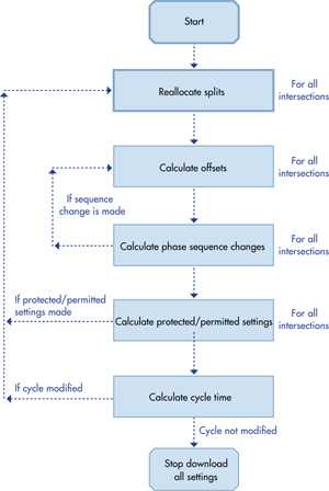
Each of these measures is used in the adaptive control algorithms as detailed in the previous sections. The five optimization stages are executed independently but in sequence and with the feedback steps as shown in figure 36. Figure 36. Chart. Flow chart of algorithms execution sequence. In step 1, the split reallocation algorithm is executed for each intersection in the system. This step identifies if any slack green time can be shifted from one or more phases to another within the current cycle time to minimize the maximum phase utilization at the intersection. Safety is evaluated by checking that the reallocation either provides a safety benefit by reducing total conflicts or that the reallocation does not exceed a prescribed threshold for the safety/efficiency trade-off value. After this reallocation, the offset adjustment algorithm is executed in step 2 to identify any modifications to the offsets to improve progression. The total capture efficiency of the offset to capture occupancy on the coordinated phases at the subject intersection and its neighbors is calculated to represent the efficiency of the proposed change. Similar to the split calculation, safety is evaluated by checking that the new offset either provides a safety benefit by reducing total conflicts or that the proposed change does not exceed a prescribed threshold for the safety/efficiency trade-off value. If either of these continues to be true, the algorithm will continue changing the offset in that direction until efficiency is degraded, safety is degraded, or a preset threshold is reached. For example, to minimize transition effects, the changes to offsets at any adjustment interval may be limited to a small value such as 5 s (or X percent of cycle). After the splits and offsets are calculated, modifications to the phase sequence (step 3) are evaluated with the new split values calculated in step 1. If any phase sequence modifications are identified that adjust the offset (the departure platoons to adjacent intersections), the offset calculation must be reexecuted to determine if this change is of further benefit and can be retained or if the change is detrimental to efficiency or safety performance. If the change is detrimental, the safety/efficiency trade-off can be used to determine if the phase sequence change should be dropped or if it is worth reexecuting the offset search algorithm to find a slightly better solution. Next, potential changes to the protected/permitted settings for left-turns are evaluated (step 4) using the phase sequence selected in the previous step. If any left-turn settings are deemed beneficial to both efficiency and safety or deemed beneficial to efficiency and within the safety/efficiency trade-off value, the split reallocation algorithm may have to be recalculated, particularly if the left-turn mode is changed from protected to permitted-only. This change, in effect, omits the left-turn phase, setting its split to zero, which frees up additional time in the cycle for other phases. It may not be the best policy to simply provide all of that split for its corresponding companion through phase (e.g., phase 6 if the left turn is phase 1). In turn, if the splits are reallocated at this step, the offsets, phase sequence, and protected/permitted settings are reevaluated as well. Finally, the cycle time adjustment algorithm is evaluated (step 5). Since cycle time affects all of the intersections in the system, it is important that this adjustment is calculated last, after all of the improvements to individual locations are calculated. As with the phase sequence and protected/permitted settings, if it is deemed beneficial to modify the cycle time, the other algorithms must be reevaluated within the new value for the cycle. 6.5 PHASE 2 RESEARCH APPROACHThe plan for research in phase 2 of the project is as follows:
Validation of the approach with long-term crash studies will be done in phase 3 after the proof-of-concept demonstration. 6.5.1 Task 1: Develop the Safety Performance Function In this task, the designed experiment will be specified in more detail than provided in this initial plan, and the simulations of the designed experiment will be run to collect the necessary traffic conflict data on the impact of interactions between the input parameters. Approximately 10 percent of the runs will then be set aside for the theoretical validation process in task 2. The remaining runs will be used to calculate the regression coefficients of the safety performance function. Several functional forms of the regression equation will be tested according to the results of the regression process. It is typical in regression modeling that some variables that were hypothesized to have significant impact turn out, in fact, to have very weak influence on the performance. These variables are then removed from the model, and the coefficients are recalculated. 6.5.2 Task 2: Validate the Safety Performance Function In task 2, the predictive performance of the safety function will be tested with the ~10 percent of the simulation runs that were held out of the regression process. This step is important to identify the ability of the safety performance model to closely replicate the data obtained directly from running a particular simulation case. If the performance of the model is insufficient, it may be necessary to revisit the variable selection and regression form steps completed in task 1. 6.5.3 Task 3: Develop the Multiobjective Adaptive Algorithms In task 3, the adaptive control algorithms specified in sections 6.3 and 6.4 will be implemented in software. These algorithms require both detector and phase-timing data as described in each section. This data will be obtained from a microscopic simulation model. The data-processing and evaluation concepts from ACS Lite for split tuning and offset tuning (and cycle time tuning, if it is available when the phase 2 project begins) and the evaluation of the safety performance function and additional tuning steps as outlined in sections 6.3 and 6.4 will be added. The other algorithms, for phase sequence selection and protected/permitted operation, will be new developments, and a new communications processing component will be developed to avoid any proprietary issues with Siemens ITS, the developers of ACS Lite for FHWA. 6.5.4 Task 4: Evaluate the Performance in Offline Scenarios In this task, microsimulation data will be obtained for several test cases and will be output to files. These data files will be input to the adaptive control calculation engine to verify that the compromise algorithm process executes as expected. Since there is no feedback loop to the simulation process, the results of the changes to the traffic signal parameters cannot be assessed for the real performance, so this task will simply demonstrate that the algorithms are functioning. 6.5.5 Task 5: Implement the Algorithms in a Real-Time Processing System In this task, the algorithms will be implemented in an online manner with a traffic simulation model in the loop. To streamline the process of moving the algorithms to real-world testing, the algorithms will be interfaced to a virtual traffic controller that is identical to the version of the controller that runs in the field. There are two such controllers available in the market today: D4 from 4th Dimension Traffic and the Econolite ASC/3. Both are able to interface to the VISSIM® microsimulation model environment. Currently, the research team has more experience with the D4 virtual controller, but it will consider both as part of the project. In either case, the interface between the optimization component and the field controller will be an open standard such as the National Transportation Communications for Intelligent Transportation Systems Protocol. This implementation will allow evaluation of the performance of the algorithms before deployment in the street. A similar architecture is envisioned for the system when deployed in the real world. The adaptive control algorithms will reside as part of a central system, similar to the architecture of ACS Lite, by polling detector data and phase timing information from the controllers and downloading new timing parameters on a periodic basis (every 3–5 cycles). This adaptive control component will be part of a central system, unlike ACS Lite, which operates as a master controller. 6.5.6 Task 6: Test the Algorithms' Performance in Simulation Scenarios In this task, the algorithms will be tested in simulation scenarios. A combination of scenarios for single intersections, small arterial, long arterial, and small networks will be tested. The test cases will replicate field locations that will be candidates for field testing in task 7. The simulation test results will be tabulated and used both to determine if it is worthwhile to deploy the system in the real world and to evaluate its online performance. 6.5.7 Task 7: Show Proof of Concept in a Limited Field Deployment Assuming acceptable performance of the system in task 6, task 7 will deploy the algorithms to the field to assess their performance in the real world. Since the development of the system in task 5 uses the virtual controller software, there should only be minor modifications necessary to deploy the approach at real intersections. A possible test includes perhaps three to five intersections being controlled by the adaptive system. Before- and after-travel time runs and traffic conflict analysis studies would be executed to evaluate the system performance. The site could then be used for long-term data collection and performance analysis in phase 3. |
||||||||||||||||||||||||||||||||||||||||||||||||||||||||||||||||||||||||||||||||||||||||||||||||||||||||||||||||||||||||||||||||||||||||||||||||||||||||||||||||||||||||||||||||||||||||||||||||||||||||||||||||||||||||||||||||||||||||||||||||||||


 s earlier, or adjust to
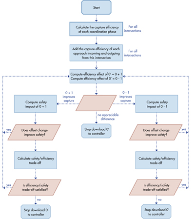
 .
.
 .
.