
6/1/2018
Also available as Adobe PDF (1.8 MB)

Notice
This document is disseminated under the sponsorship of the U.S. Department of Transportation (USDOT) in the interest of information exchange. The U.S. Government assumes no liability for the use of the information contained in this document.
The U.S. Government does not endorse products or manufacturers. Trademarks or manufacturers’ names appear in this report only because they are considered essential to the objective of the document.
Quality Assurance Statement
The Federal Highway Administration (FHWA) provides high-quality information to serve Government, industry, and the public in a manner that promotes public understanding. Standards and policies are used to ensure and maximize the quality, objectivity, utility, and integrity of its information. FHWA periodically reviews quality issues and adjusts its programs and processes to ensure continuous quality improvement.
1. Report No. FHWA-HEP-18-065 |
2. Government Accession No. |
3. Recipient’s Catalog No. |
|||
|---|---|---|---|---|---|
4. Title and Subtitle Noise Measurement Handbook |
5. Report Date September 15, 2017 |
||||
6. Performing Organization Code |
|||||
7. Author(s) RSG |
8. Performing Organization Report No. |
||||
9. Performing Organization Name and Address RSG 55 Railroad Row White River Junction VT 05001 |
10. Work Unit No. (TRAIS) |
||||
11. Contract or Grant No. |
|||||
12. Sponsoring Agency Name and Address U.S. Department of Transportation 1200 New Jersey Ave. SE Washington, D.C. |
13. Type of Report and Period Covered |
||||
14. Sponsoring Agency Code |
|||||
15. Supplementary Notes Other authors: Bowlby & Associates, Inc.; ATS Consulting; Environmental Acoustics; Illingworth & Rodkin |
|||||
16. Abstract This handbook provides best-practice guidance on recognizing which measurement methodologies apply to which project type (Section 1.0), how to plan a noise measurement program (Section 2.0), descriptions of measurement methodologies and related considerations (Sections 3.0-15.0), terminology (Section 16.0, Appendix A) and measurement instrumentation (Section 17.0, Appendix B) related to highway traffic noise, example report documentation for measurements (Section 18.0, Appendix C), and supporting material for various methodologies (Sections 19.0-21.0, Appendices D-F). Sections 3.0 and 4.0 are directly applicable to the conduct of traffic noise studies required by the Federal Highway Administration (FHWA) noise regulation in 23 CFR 772. Section 22 is a bibliography. The information provided in this handbook is based on the 1996 FHWA Measurement of Highway-Related Noise, and is based upon current national and international standards and practice updates. This handbook should be viewed as best-practice guidance and not direction as to how the work must be done. Some project sponsors have established and use their own procedures, which typically would be followed in the event of a conflict. |
|||||
17. Key Words Highway traffic noise, Noise measurement methodologies; traffic noise studies, noise regulations, best practices |
18. Distribution Statement |
||||
19. Security Classif. (of this report) Unclassified |
20. Security Classif. (of this page) Unclassified |
21. No. of Pages 188 |
22. Price |
||
Form DOT F 1700.7 (8-72) Reproduction of completed page authorized |
|||||
Noise is an important environmental consideration for highway planners and designers. Transportation agencies measure different aspects of highway noise to determine or predict community impacts during urban planning or to conduct research that support their programs. Precise, uniform, field measurement practice allows for valid comparison of results from similar studies performed by a variety of transportation practitioners and researchers.
This handbook provides best-practice guidance on recognizing which measurement methodologies apply to which project type (Section 1.0), how to plan a noise measurement program (Section 2.0), descriptions of measurement methodologies and related considerations (Sections 3.0-15.0), terminology (Section 16.0, Appendix A) and measurement instrumentation (Section 17.0, Appendix B) related to highway traffic noise, example report documentation for measurements (Section 18.0, Appendix C), and supporting material for various methodologies (Sections 19.0-21.0, Appendices D-F). Sections 3.0 and 4.0 are directly applicable to the conduct of traffic noise studies required by the Federal Highway Administration (FHWA) noise regulation in 23 CFR 772.[1] Section 22 is a bibliography.
The information provided in this handbook is based on the 1996 FHWA Measurement of Highway-Related Noise,[2] and is based upon current national and international standards and practice updates. This handbook should be viewed as best-practice guidance and not direction as to how the work must be done. Some project sponsors have established and use their own procedures, which typically would be followed in the event of a conflict.

Typical highway noise evaluation projects range from Type I highway construction or reconstruction projects[3] to research supporting state highway agency (SHA) and Federal programs. Noise evaluations comprise the application of several noise measurements, and there are several measurement methodologies related to highway traffic noise. Methodology application depends on the type of highway project. This section of the guidance document lists example projects and applicable measurement methodologies and includes a brief explanation of potential applications. Some of the measurement methods are essential to the project and some are not required but benefit the project, as described below.
Table 1-1 shows the measurement methods applicable to determining operational noise impacts for Type I highway construction or reconstruction projects. Existing noise measurements should be conducted for these types of projects for two primary reasons: 1) to establish existing noise levels; and 2) to validate the FHWA Traffic Noise Model (FHWA TNM). Measurement of noise sources other than roadways/highways may be necessary for noise-sensitive areas that are exposed to multimodal noise sources such as trains and aircraft; screening estimates or prediction methods may suffice for consideration of these noise sources. Measurement of the influence of pavement on noise in areas adjacent to roadways/highways may be helpful for validating the noise model and for understanding pavement’s influence on the project. Measurement of existing vibration at highly vibration-sensitive properties, such as recording studios, concert halls, or medical or research facilities with vibration-sensitive equipment, may be warranted if a highway project results in train tracks moving within Federal Transit Administration (FTA) vibration screening distances for these types of receptors.[4] Highway traffic is typically not a vibration issue due to operational vibration source strengths and distances to structures, however, vibration measurements could be applicable if a highway has planned road irregularities (e.g., bridge joints) close to sensitive structures.
Table 1-2 shows the measurement methods applicable to noise abatement design for Type I projects. Part of abatement design includes understanding noise sources other than those from the project highway. These other sources could include nearby arterial roads, industrial noise, or train or aircraft noise sources. Establishing existing sound levels with general information about where the noise sources originate can help determine the effectiveness of a project’s mitigation design. Existing noise barriers can influence noise abatement design; validating FHWA TNM with existing noise barriers will help with noise abatement design for the project. Application of the building noise reduction measurement method is recommended for cases where building insulation is being considered for reducing indoor noise levels. Noise barrier insertion loss measurements are likely not needed for a Type I project, but there may be circumstances that require understanding the effect of existing barriers or that help establish future barrier effectiveness. Existing vibration measurements may be needed for cases where vibration mitigation is being considered.
Table 1-3 shows the measurement methods applicable to highway construction, whether it is new construction or reconstruction. If needed, construction equipment noise and vibration levels can be measured to help predict construction operational impacts, where the levels would be implemented in construction noise or vibration prediction models or methods. Also, existing noise and vibration levels can be established prior to construction; this may help to establish reasonable limits and expectations during the construction phase, particularly for receivers that may be highly noise sensitive or vibration sensitive. Construction noise mitigation might involve use of temporary noise barriers or building sound insulation. In the former case, determining noise barrier insertion loss may be desired. In the latter case, pre-insulation or post-insulation measurements could help establish interior noise levels or the effectiveness of the insulation.
Table 1-4 shows applicable measurement methods for projects that require evaluation of the need for a noise barrier on an existing highway (Type II projects[5]) or for investigation of noise or vibration complaints. Measuring the existing noise or vibration may be necessary to determine the levels in relation to project sponsor or Federal limits or recommendations. It may also be necessary to apply traffic noise modeling as part of the project, which would require model validation. In addition, to determine if an existing barrier is functioning as intended, the noise barrier insertion loss method applies.
Table 1-5 shows the measurement methods applicable to creating vehicle noise emission levels for input to the FHWA TNM. The intended application of the method is for vehicle types that differ substantially from the five standard vehicle types contained in FHWA TNM (e.g., recreational vehicles or electric vehicles). The method should not be used to input state-specific emission levels for the five standard vehicle types. Understanding the influence of the ground type at the emission-level measurement site(s) may be helpful since ground type can affect measured emission levels; this can be accomplished by applying a method that measures the ground’s influence.
Table 1-6 shows the measurement methods applicable to determining the effectiveness of highway noise barriers. The insertion loss can be measured/calculated for both an existing noise barrier or for a project where a barrier will be installed (methods would be applied to pre- and post-installation). An element of insertion loss is the loss of soft-ground effects: sound-absorbing ground surfaces that reduced highway noise prior to barrier installation may no longer contribute after installation due to the sound propagation path being raised well above the ground and over the top of the barrier. Apply these methods to measure the effect of soft ground. Part of determining a barrier’s effectiveness may include examination of other noise sources and their influence on the received noise level.
Table 1-7 shows the measurement methods applicable to determining the influence of pavement on highway noise. Several methods are available, and the chosen method may depend on the volume of traffic on a highway, measurement site quality, or study goal. A combination of methods would provide the most comprehensive information. A method that measures tire-pavement noise is relatively inexpensive in terms of data collection and analysis costs. These methods allow mapping of sound levels on highways or highway systems or on single project areas or can be applied to evaluate consistency in pavement construction. These methods can also supplement the vehicle noise or traffic noise measurement methods (wayside methods, measured on the side of the road). The wayside methods focus on single points along a road; these methods account for propagation effects (to various degrees) and are intended to capture noise that would be experienced by sensitive receptors. Measurements can also help determine the influence of pavement or ground on sound propagation; these can help in understanding or predicting wayside noise levels (when combined with tire-pavement noise measurements). All these methods can help with pavement ranking and longevity research. Conducting vehicle interior noise measurements could help evaluate interior noise produced by different pavements and by pavement surface modifications such as rumble strips.
Table 1-8 shows the measurement methods applicable to evaluating the validity or accuracy of a highway traffic noise model (such as FHWA TNM). Of primary importance is to conduct existing noise measurements specifically for model validation. In addition, pavement or ground adjacent to a highway may influence received sound levels; various measurement methodologies can evaluate these effects. Lastly, noise from other transportation sources and their influence on existing noise measurements needs to be established; existing noise measurements that include such sources would not be predicted by FHWA TNM and may lead to existing noise levels exceeding predicted levels when comparing for accuracy.
Table 1-9 shows the measurement methods applicable to US Department of Housing and Urban Development (HUD) projects. HUD noise assessments are required when using Federal funds or loan guarantees for building projects near transportation facilities.[6] For these projects, predictions are made for the combined noise levels for highway, rail, and aircraft noise sources. For cases where there is insufficient traffic data or not-easily-modeled noise sources, HUD gives some consideration to the use of measured sound level, although HUD guidance should be sought before presuming that measurements will be allowed to be used.[7] Associated noise levels can be acquired through methods outlined in this guidance document for highway traffic noise and other transportation noise sources.
Noise study success is predicated on proper planning. Many of the planning steps are similar regardless of the type of measurements being taken, but some types of measurements require unique planning. For consultants, planning for required measurements is often done at the proposal stage, where coordination with the project sponsor is recommended for developing a well-defined scope and realistic schedule. The number of sites or types of requirements can change (such as having to abort and reschedule measurements due to unacceptable weather conditions). Importantly, planning a measurement study requires consideration of a project sponsor’s requirements, the number of sites and measurement durations, travel time to and from the project area, time on site and between sites, and staffing to estimate study duration and the associated labor and travel. The steps outlined in this handbook represent best-practice guidance; however, this guidance is not meant to override a project sponsor’s procedures.
It is important that the person planning the study articulates the purpose of the measurements, including the sound source of interest and the needed measurement procedure, in order to: 1) plan properly for the measurements; and 2) help ensure that there is agreement and understanding with the person approving the study and the persons conducting the measurements. For example, for a Type I noise study (per 23 CFR 772), is the project on new alignment (Section 3.0)? If so, it may be difficult to establish a worst noise hour for the existing situation because there may be no existing roads near the area to be measured. The FHWA noise regulation says that the noise study should be done for the worst noise hour in the future design year for the “build” condition. However, for a new-alignment project, do not assume that the worst hour in the existing condition correlates to the worst hour in the build condition. Or, is the project a widening of an existing road, in which case measurements for model validation do not need to be done during the worst hour and are best not done under congested traffic conditions (Section 4.0)? Is the source the overall ambient sound (Section 3.0) or only the traffic on the road to be widened (Section 4.0)? What are the spatial and temporal natures of the source(s) of interest and the other sources that may be a part of the measurement or that may interfere with the measurement? How will those natures affect the decisions of when to measure and how long to measure? The measurement procedures in this handbook address these and other questions.
Properly identify the study area to ensure that all receptors of interest are considered in the selection of noise measurement sites. Identification begins with reading and understanding the Scope of Work, the Purpose and Need Statement, and, if applicable, the identified logical termini of the overall project. Per 23 CFR 772.5, “If a project is determined to be a Type I project under this definition then the entire project area as defined in the environmental document is a Type I project.” In the case of a Type I project, the study area may encompass many miles of existing and proposed highway and may include several alternative alignments through the study corridor. A study area may be divided into several areas with similar noise characteristics; often by community, neighborhood, or other receptors of interest that are in close proximity to each other. Alternatively, the study area may be limited to a single land use—such as a school—that requires building noise reduction measurements. A study “area” could also comprise multiple locations along different highways in different parts of the region, state, or country. Examples of this situation include regional or statewide Type II noise barrier needs studies or national noise barrier insertion loss or vehicle noise emission levels research studies.
In many cases, highway plans and local mapping are helpful for understanding the project limits and for determining whether certain possible receptors of interest have been identified for acquisition by a project sponsor for project right-of-way (ROW). Project plans and mapping may be obtained from the planning and design offices of the project sponsor or the environmental or design consultants responsible for the study area or project of interest. County geographic information systems (GIS)—where available—are excellent sources of mapping, and often include a 5-ft or 2-ft (1.5-m or 0.6-m) ground elevation contour data layer. More information on geospatial and elevation data useful for noise modeling (and possibly for noise measurements) is available in FHWA’s Recommended Best Practices for the Use of the FHWA Traffic Noise Model (TNM).[8]
For existing noise studies for Type I highway projects, land-use mapping will help identify the activity category of the adjacent or nearby land uses, which in turn identifies how or if those land uses need to be studied. In some cases, such as noise barrier insertion loss measurements, highway plans and off-ROW ground elevation contour mapping are critical for finding an “equivalent” No-Barrier site (“BEFORE”) for simultaneous measurements at the Barrier site (“AFTER”).
The type of measurement, as described in the various sections of this handbook, and the extent of the project area are factors that will determine the number of required noise measurement sites. Online mapping websites or programs utilizing online maps and aerial photography are essential tools in the preliminary identification of measurement sites before going into the field. These tools, including street-level photography, are useful for identifying land uses and possible areas of frequent human use that may affect or determine microphone location once on site. These tools are also useful for identifying important sources of noise that may establish the existing sound levels at a site in the case of a Type I new-alignment project. In addition, these tools can help identify undesirable noise sources that interfere with a needed measurement of traffic noise only, such as for FHWA TNM model validation or noise barrier insertion loss determination. Assess the presence and potential impact of these sources during a field review.
Online resources, as useful as they are, are not always kept current and should not be relied upon as sole sources of site information when planning a study. A field review is important as the final step for deciding on the suitability of a measurement site and for determination of the best location to place the microphone. However, especially for smaller Type I studies, it may not be practical in terms of travel, labor and cost to undertake an advance field review. Make final determinations in consultation with the project sponsor.
Some project sponsors require consultants to conduct a field review for site identification and to submit a report or letter requesting approval of proposed measurement sites before mobilization for measurements. Some project sponsors have their own staff conduct the field review with the study consultant and approve the locations in the field. Others rely on information from a desk review for site approval. Still other project sponsors do not require any advanced approval of the sites, relying instead on the judgment of the consultant or measurement team for site selection during the planning stage, with confirmation during the noise measurement trip.
Identifying set-up problems when the field crew arrives on site to do the measurements is the least desirable situation. Field reviews are critical before mobilizing for measurements on major research studies with more complex measurement set-ups requiring greater attention given to the details during project planning—in advance of, during, and after the field review. Wait until after considering all details to make a final selection of sites and rule out sites that are no longer suitable. Early identification of set-up problems makes it easier to find solutions, alternative sites or alternative microphone locations.
Access to the microphone location(s) is critical. Some questions to consider when selecting measurement sites are: Where can gear be dropped off safely for deployment? How difficult is the path between the drop-off point and the microphone locations? Must brush or tall weeds be cut to clear a path? Are fences impeding access, requiring ladders or other means to cross? Are there gates that are locked and, if so, is a key available or is there another way around? Where will vehicles be parked during the measurements?
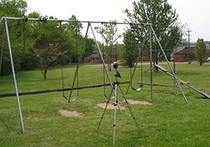
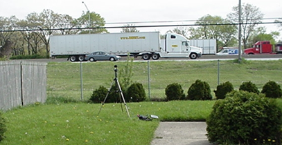
Microphone heights need to be determined (such as atop a noise barrier for insertion loss measurements); it is also important to determine the support method(s) for elevating and holding the microphones at desired heights. Methods for stabilizing and securing the microphone support (such as weighing down the base or using guy wires) need to be addressed. Considering where the analyzer and operator will be located can help determine microphone extension cable lengths If a meteorological station is being used, then similar considerations need to be given to transducer support, cabling, and instrumentation placement. Finding acceptable and safe sites can be a challenge for projects requiring traffic counts or speed measurements.
Developing site layout and set-up sketches ahead of the field review—and then finalizing them during the field review—is a good practice. Likewise, creating site evaluation data sheets that can be completed during the field review helps with thinking through issues that are critical to successful measurements. On a complicated set up, determining the exact points to place tripods and marking them for easy identification during the measurement trip can expedite the set-up time and mitigate uncertainty and errors. Taking photographs from several directions and narrated videos of potential microphone locations, the surrounding terrain, noise sources, and the roadway pavement may be valuable for the field crew and in developing final plans.
Some projects require access to private property (residential or otherwise) to conduct noise measurements (and to plan research-oriented studies). Field crews may also need access to public properties such as school yards or buildings. There are varying requirements for obtaining access permission. For research-oriented studies, such as noise barrier insertion loss measurements, obtaining advance approval is critical because the success of the measurements may depend on accessing a specific piece of property.
Some project sponsors require notice to property owners requesting permission or providing notifications of intent to enter on sponsor letterhead. Other sponsors have less strict requirements and may not require notice, just a simple courtesy knock on the doors of residences or businesses requesting access upon arrival at a planned site. Some locations may require additional arrangements such as when there is a locked gate. If access permission is given, then carrying a name and phone number for the contact person on the property is a good practice in case entry is not successful.
Approval is often sought during the pre-measurement field review and could include leaving a letter with a phone number to call in case no one is on site at the time of the first visit to give permission. Having a letter of identification (during the field review and during the measurements) is helpful. The letter could briefly describe the need for access, what will be done (e.g., “setting up a camera tripod with a sound level measuring system in the backyard for a half-hour”), the expected date and time range (e.g., “daylight hours,” “between 10:00 p.m. and midnight”), and project sponsor contact information to confirm the legitimacy of the request or to obtain more details. The inability to obtain or be granted permission to enter private property usually requires choosing another site.
In some cases, setting up on private property can be avoided by staying on public property at a nearby location that will provide similar sound levels results, such as a local street’s cul-de-sac that ends at the ROW fence where the distance to the road in question is the same as the distance to the residential yard of interest. On the other hand, if there is a house at the end of that cul-de-sac and a backyard measurement is needed, then setting up in the cul-de-sac in front of the house would not give comparable results.
In other cases, measurements will need to be made on the highway ROW. Examples include vehicle noise emission levels at 50 ft (15.2 m) from the center of the near lane or the reference microphone atop a noise barrier in an insertion loss study. Project sponsor requirements to access these locations vary, possibly including approval for a roadside safety committee that might require formal input and approval at a regularly scheduled meeting. In other cases, a ROW access permit may be required from the responsible official. In still other cases, approval may be less formal. Regardless, seek permission in advance to avoid schedule delays and possible loss of a needed measurement location.
Each measurement procedure in this handbook will have different personnel needs and, in many cases, different equipment needs. Assess and address these needs during the planning process. Some measurements, such as existing sound levels for a new-alignment highway, can be done by one person (or more than one person, each with their own noise measurement equipment so that multiple sites can be measured at the same time).
Other measurements require more people. For example, model validation measurements may require additional people to count traffic and collect vehicle-speed data simultaneously with the sound level measurement; however, if traffic is being video-recorded for counting in an office later, then the field crew size can be reduced. Research-oriented measurements, including noise barrier insertion loss measurements with simultaneous measurements at the Barrier and equivalent No-Barrier sites, could require three or four people to deploy the sound level and meteorological instruments and attend the sound level instruments during the data collection, plus another crew to count or record traffic and collect speed data.
Also assess equipment needs. Each section of this handbook describes the needed equipment and Appendix B provides detailed information on instrumentation, accessories, and field supplies. Planning for contingencies by including back-up equipment can be important, especially if the measurements are complex, not easily replicated or far from the home base, and if replacements are not easily obtained in the field if something goes wrong.
Developing a detailed tentative field schedule will facilitate effective budgeting. Consult with the field crew if the person planning the study does not typically go into the field for measurements. Include the following in a field schedule:
The amount of time needed to download, label and store data depends on the type and complexity of the measurements. No special planning is needed for single-instrument set-ups; however, consider having a file labeling and storage protocol for consistency across jobs. Research measurements with multiple sound level instruments may require many files for each measurement period:
Use a logical file naming system—including site number and microphone or other transducer number, date, time, and type of file—for data reduction and analysis after the measurements.
Travel arrangements are part of the planning and budgeting process. Consider the following when making travel arrangements as part of the planning and budgeting process:
Pre-trip equipment gathering, testing, and settings: Check equipment functionality and settings (typically A-weighting and one-minute sampling interval duration) before starting travel. Verify functionality of accessories and that batteries are of the right type and are fresh or charged. Synchronize all personal watches or time devices and the time clocks in the instruments before the measurements begin; a useful online time reference is at www.time.gov. Verify packing of all supplies to be carried or shipped to the site.
Development of field data sheets: The FHWA Noise Measurement Field Guide includes sample field data sheets and logs.[9] Use these or similar sheets and logs. Templates of field logs or data sheets may also be customized for each job, perhaps with some common information, such as project name and location, pre-filled. Each section of this handbook contains field data documentation information.
Tracking weather forecasts: The ability to collect valid sound level data depends on weather conditions. High winds and precipitation are leading causes of delayed, interrupted, rescheduled, or cancelled sound level measurements. Online weather sites are good resources for monitoring forecasts. The field crew should monitor weather conditions until the time of departure before making the decision to travel.
Two final notes:
The main use of the procedures in this section is to determine existing noise levels for a proposed highway project on new alignment. They could also be used for other basic noise measurements such as:
The FHWA noise regulation in 23 CFR 772 requires the determination of existing noise levels for highway noise studies to establish a base case for comparison with future project noise levels. Comparison of existing and future noise levels is one of two means of determining the noise impacts of a proposed project, that is, by identifying whether there is a substantial increase in level due to the project.
Section 772.11(a) of 23 CFR 772 requires “determination” of existing noise levels[10] by:
This section of the handbook discusses field measurements for new alignment projects, and Section 4.0 discusses model validation noise measurements for the second approach.
For projects on new alignment, the noise analyst identifies project impacts by comparing existing noise levels to future worst-hour noise levels for the design-year “build” condition, which are predicted using FHWA TNM. (The analyst also compares those future levels to activity-based Noise Abatement Criteria (NAC) in 23 CFR 772.) In 23 CFR 772.5, the term “existing noise levels” is defined as “the worst noise hour resulting from the combination of natural and mechanical sources and human activity usually present in a particular area.” These sources could include traffic on nearby or distant roads that are not part of the project, as well as noise from other modes of transportation, and noise from non-vehicular sources. It may be difficult to establish a worst noise hour for the existing situation for a new-alignment project because there may be no existing roads near the area to be measured to create a repeatable noise environment. In any case, do not assume that the worst noise hour in the existing condition correlates to the worst noise hour in the build condition.
Site selection for measurements is driven by the study goals—in this case, establishing existing sound levels to assess impacts based on the future increase over those levels due to a highway project. Specifics may depend on a project sponsor’s noise policy or procedures.
There are two considerations regarding site selection:
Site selection is guided by the location of noise-sensitive receptors and major nearby noise sources. Land-use maps, aerial photos, including web-based mapping sites and field reconnaissance are helpful for initially identifying potential noise-sensitive areas. Budget and schedule restrictions preclude measuring at all receptors; even without these limitations, measurements at all—or even most—receptors are not necessary or expected.
Include residential areas in a noise measurement study. Consider the representativeness of each site during the selection process. In some instances, one residential site near a proposed highway can represent other similar sites—especially in the case of new alignments where there may not be a nearby major roadway. In any case, the representative site should exhibit similar background sound level conditions to the other sites. Consider measurements at other noise-sensitive land uses identified in the activity categories in 23 CFR 772.
Site selection is also guided by other noise sources that may raise the “typical” existing level at a site such that the increase in level due to the highway project would be less than otherwise; this increase in levels could affect a decision on the noise impact at a site. Address the frequency of occurrence and duration of noise from these other sources in the context of the hourly time period considered in highway noise studies. Examples of these other sources to be aware of include industrial or manufacturing sites, railroads, airports, even especially loud air conditioning or pool pumps in residential areas.
Usually, study objectives will dictate microphone locations. Measurements on residential property are usually taken in an area in the yard between the proposed ROW line and the building where frequent human activity occurs, such as a patio, porch, pool, deck or swing set. In general, choose measurement sites that are clear of obstructions and vertical sound-reflecting surfaces. However, an area of frequent human use often has nearby reflecting surfaces, such as the building wall, and a measurement may need to be made at that location. A reflecting surface can cause an increase in the measured sound level compared to the surface not being present, depending on the location of the major sound sources relative to the building and the microphone. In these cases, the reflected sound level increases due to reflections at these areas of frequent use represent reality.
Lacking easily identified areas of frequent human use, choose a point near the center of the yard for smaller lots. For larger lots, a location closer to the residence than the center of the yard may be more appropriate. Avoid extreme locations—either too close to the road or too far from it—to not understate or overstate noise levels and noise impacts. In choosing locations, be aware of localized noise sources that would affect or contaminate the measured levels, such as air conditioners, playing children, and dogs. Consistency in microphone locations is desirable, allowing for site conditions to dictate deviations. Also, it may be possible or necessary to choose a location on public ROW that is representative of the noise environment at the area of frequent human use if private property access is a problem. In such a case, be especially aware of localized noise sources such as street traffic.
In general, use a microphone height of 5 ft (1.5 m) above ground, being representative of ear height for a standing person. For multistory apartments with outdoor balconies or single-family homes with outdoor decks, then microphones at heights of 5 ft (1.5 m) above floor elevation may be needed.
Per 23 CFR 772 for an Activity Category C land use, if no exterior activity exists at a site or is far from or shielded from the project, there may be a need to study the interior environment as an Activity Category D land use. Section 6.0 provides a procedure for measuring an outdoor-to-indoor building noise reduction that could be applied to a future exterior sound level prediction to determine a future interior sound level. The guidance on interior microphone placement in Section 6.0 could also be used in conjunction with the procedures in this section for direct measurement of an existing interior sound level for comparison to a future interior predicted sound level for impact assessment per 23 CFR 772.
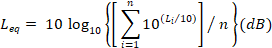
For determining existing noise levels per 23 CFR 772, the needed descriptor is the one-hour A-weighted equivalent sound level, Leq(h), or the A-weighted sound level exceeded 10% of the study hour, L10(h). While not required for a Federal-aid noise study being done with Leq(h), L10(h) is also a useful descriptor because the L10(h) - Leq(h) difference provides clues about the amount of variation in the levels during the sample period. For example, a small difference means little variation in the level over time. Typically, for many highway traffic situations, Leq(h) is 2–3 dB lower than L10(h), whereas Leq(h) being greater than L10(h) typically means a low traffic volume. Also of potential interest are: L50 (the A-weighted sound level exceeded 50% of the measurement period), an indicator of the median sound level; and L90 (the A-weighted sound level exceeded 90% of the measurement period), an indicator of the background sound level. The maximum A-weighted sound level (LAFmx) is the loudest sample in the measurement period, and can be an indicator of possible measurement anomalies, such as unrepresentative loud events or equipment problems.
For existing noise measurements, the key instrumentation and accessories include the following:
Appendix B provides information and a discussion on instrumentation and other useful accessories and field supplies.
For this section—determination of existing noise levels by field measurements for projects on new alignment—traffic-counting and speed detection devices are typically not needed because there is usually not a road present for which traffic data are needed for model validation. However, traffic classification counts on nearby local roads can provide insight into the measured sound level and important nearby noise sources.
Consider three factors when selecting a sampling period:
In general, per 23 CFR 772, the goal of this part of a noise study is to determine existing noise levels in terms of Leq(h) (or L10(h)). As noted above, existing levels are to represent the worst noise hour, yet for new-alignment projects that hour may not be easily identified. The worst noise hour is generally the loudest hour. If the measurement site is near a congested highway, peak travel hours may not be the loudest hours. Near a highway, the loudest conditions are usually caused by the highest traffic volume at the highest average speed, which could easily be outside the rush hour periods—when traffic is free-flowing and when heavy truck volumes tend to be higher.
If the congested road is the subject of the proposed project (i.e., it is to be widened), then follow the guidance in Section 4.0 (model validation measurements) instead of the guidance presented in this section. However, if that road is not part of the project, but it is influencing the sound levels at a receptor under study, then use the guidance provided in this section.
In many cases, both with and without a major road nearby, the worst noise hour will occur between 6:00 a.m. and 7:00 p.m. It is often useful to have at least one site where the sound level instrument can be left out throughout those hours to help identify the worst noise hour. A 24-hour measurement at one of the project’s noise study sites could be made to understand better the diurnal variation in the sound level; however, 24-hour sampling is not required for determining existing noise levels for the purposes of 23 CFR 772. A 12-hour to 14-hour measurement at one representative location could be useful in identifying the worst noise hour at that location, but be aware that, depending on local noise sources, the worst noise hour at that location may not represent the worst noise hour at other locations along the corridor for a new-alignment project. In any case, do not assume that the worst noise hour for existing condition is the same as that for the future “build” condition.
A second aspect of the “when to measure” question pertains to meteorological conditions, which can substantially affect measured sound levels. First, do not make sound level measurements during precipitation or when the pavement is wet. Aside from being bad for equipment, rain drops can generate noise on leaves, metal roofs, and plastic bags that have been placed over microphone windscreens and instruments. Tire noise increases on wet pavements, especially in the higher frequencies that most affect an A-weighted sound level. Second, wind affects measured sound levels in two ways:
Ideally, make sound level measurements when winds are as calm as possible when determining the existing noise environment. In any case, document wind speed and direction.
Third, the changing of temperature with height above the ground (“temperature lapse rate”) can have a major effect on measured sound levels by refraction, especially at larger distances from a source.[13] When traffic noise is part of the existing noise being measured, sound levels from that traffic will be lower during bright, sunny days (temperature profile decreasing sharply with height above ground) compared to a cloudy day or neutral atmosphere (no change in temperature with height, a condition usually only seen briefly around sunrise and sunset) for the same traffic volume, speed, and vehicle mix. While nighttime measurements are typically not made for the purposes of this section, those same traffic sound levels would be higher on clear, calm nights during inversions (temperature profile increasing with height above ground) compared to daytime levels.
Cloud cover observations may be useful in assessing the potential for temperature refraction effects. Table 3-1 shows cloud cover classes. Class 1 has the least likelihood of temperature refraction, being closer to neutral temperature profile than other conditions. Class 4 has the greatest chance of refraction that could cause the largest decreases in level compared to neutral conditions, while Class 5 has the greatest chance of refraction that could cause the largest increases in level compared to neutral conditions. Avoiding measurements before sunrise or after sunset will typically bypass inversion periods. Measurement of temperature at two heights above ground, such as 5 ft and 15 ft (1.5 m and 4.6 m), is a precise way to determine lapse rate and the likelihood of refraction, but this is not required for the determination of the existing noise levels called for in 23 CFR 772.
| Class | Description |
|---|---|
| 1 | Heavily overcast |
| 2 | Lightly overcast: either with continuous sun or the sun obscured intermittently by clouds 20% to 80% of the time |
| 3 | Sunny: sun essentially unobscured by clouds at least 80% of the time |
| 4 | Clear night: less than 50% cloud cover |
| 5 | Overcast night: 50% or more cloud cover |
Section 4.1.1 provides more information on meteorological effects on sound levels.
In choosing a measurement duration, a key consideration is the ability to represent the one-hour Leq with a shorter-term measurement to reduce time and cost for the measurement study without sacrificing accuracy. How long to measure depends on how much the sound level fluctuates.
As background for both this section (new alignment projects) and Section 4.0 (widening projects), ANSI/ASA S1.13-2005 (R2010)[15] provides useful guidance on classifying the temporal characteristics of environmental sound. It notes that sounds can be broadly classified as “continuous” or “intermittent,” and each class can be further defined as “steady, fluctuating or impulsive.” It notes that “ambient sound itself is always taken to be continuous.”[16] The differentiation between “steady” and “fluctuating” is whether “the A-weighted sound level measured with the slow exponential time weighting varies by more than ±3 dB about its mean value over the observation period.” It defines “intermittent sound” as “a sound whose sound pressure level (SPL) equals or drops below that of the ambient sound at least two times during the observation period.”
For sites where there are no roads nearby, sound levels can be relatively constant, but can fluctuate over the day, falling into “steady continuous” or “fluctuating continuous” classes. For most highway traffic noise situations (e.g., a nearby road that is not part of the project or a road that is to be widened as part of the project), the sound would be characterized as “fluctuating continuous sound.” For sites close to a highway, levels can fluctuate a great deal, depending on the traffic flow and distance from the road. The fluctuation can be small (under 10 dB) for a busy highway, especially beyond 200 ft (61 m) from the road; in closer, the fluctuation for that same road could be greater (10 dB to 30 dB), especially due to the noise from heavy truck pass-bys.
The fluctuations can exceed 30 dB close to a lightly traveled, low-volume road where there are gaps in the passing traffic that allow the sound level to drop down toward the ambient level, in which case the sound would be classified by ANSI/ASA S1.13-2005 (R2010) as “fluctuating intermittent” sound. In such a situation, ANSI/ASA S1.13-2005 (R2010) defines the “signal between the start and end of the intermittent sound” as “a sound event or simply an event.” Examples would be individual vehicle pass-bys or aircraft flyovers.
Separately, especially in low-volume situations, a key question to try to answer while in the field is whether the traffic passing during the measurement is representative of the hourly flow (e.g., one heavy truck passing by during the measurement on a road where few pass in the entire day could skew a measurement). In such a case, consider extending the sampling period.
Similarly, several unusually loud vehicles during a measurement near a lightly traveled road can skew the results of a shorter-duration measurement. On the other hand, along busier roads, loud vehicles should not, in general, be viewed as unrepresentative; they are part of the overall vehicle population, which includes a wide range of vehicle noise emission levels.
One guide for choosing duration is the greatest anticipated or observed range in the minimum and maximum sound levels occurring at the measurement site during the worst noise hour:
Additionally, most integrating sound level meters allow observation of the cumulative Leq during a measurement, even if the data are being accumulated in 1-minute intervals. If the cumulative Leq fluctuations do not settle down after measuring for the above durations, consider extending the sample period.
Consider the following when determining measurement frequency:
A single sound level measurement, regardless of its duration, only offers a slice or snapshot of the time-varying sound level at a site. Changes in traffic on nearby roads and changes in meteorological conditions, especially wind direction and temperature lapse rate around sunrise and sunset can change sound levels—sometimes substantially—as described earlier. In many cases for new-alignment projects, there may be no clear indication of noise sources that would establish an identifiable, repeatable worst noise hour. As noted above, a longer-term measurement at one site may help identify the worst noise hour at that site, but it may not be applicable to other sites. One approach for dealing with the uncertainty of worst noise conditions is to measure at each site during two different times of the day (or on two different days). If the measured Leq for the two measurements are within 3 dB of each other, arithmetically average them and round off to a whole number. If the Leq differ by more than 3 dB, there is some cause of the variation. Measure a third time and then average the closest two of the three Leq values and round off to a whole decibel.
This section presents the measurement procedure. More specific details for the person going into the field are in the FHWA Noise Measurement Field Guide. Prior to traveling to conduct the sound level measurements, plan the measurement study as described in Section 2.0.
The steps below describe what needs to be done upon arrival at the site, on through the successful collection of data.
Documentation is an essential part of every measurement. There are two stages to documentation: 1) in the field; and 2) after data analysis. This section describes field documentation. Field data sheets and more specific guidance are in the FHWA Noise Measurement Field Guide. Complete data sheets in the field while at the site. Make documentation sufficient for another person to return to that same microphone location and repeat the measurement with the same equipment and settings and under the same conditions. Here are some parameters to document using data sheets:
Typical data analysis and reporting procedures include these steps:
As noted in Section 3.0 the “determination” of existing noise levels is required in 23 CFR 772 for a highway noise study to establish a base case for comparison with future project levels. Section 772.11(a) of 23 CFR 772 requires “determination” of existing noise levels[17] by
This section discusses the measurement of noise levels for use in validating an FHWA TNM model run of the existing condition. Validation is done by comparing the predicted existing levels to the measured noise levels. These measurements are only intended for validation of runs for particular highway project noise studies and not for use in an overall validation study of FHWA TNM.
Measurements made for model validation do not have to be made during the worst noise hour. The purpose of these measurements is not to define the existing noise levels for impact determination, but to allow validation of the existing model run so that FHWA TNM can then be used with some degree of confidence to predict the existing worst noise hour levels that will be used in impact determination.
Obviously, an existing highway needs to be present to validate the model. The validation process includes simultaneous collection of sound level data, traffic classification counts, and traffic speed data; it also includes details on the type of pavement, the ground type, terrain and other potential sound-attenuating features between the road and the microphone.
These data are all used to create a model run within FHWA TNM, with the counted traffic factored up to hourly volumes for each vehicle type. Each measurement will have its own FHWA TNM validation run with the counted traffic specific to the measurement period.
The predicted sound levels are then compared to the measured sound levels for the same periods. The FHWA Highway Traffic Noise: Analysis and Abatement Guidance[18] notes the following:
“If the measured and predicted highway traffic noise levels are within +/-3 dB(A) for measurements taken at an NSA [noise-sensitive area], then the model is considered valid and can be used to predict existing highway traffic noise levels for that NSA. If the model is not within +/- 3 dB(A) for all the measurements, then the model is not considered valid until additional measurements are made or until the analyst identifies the reason for the discrepancy and makes a correction within the model. In some circumstances, it is not possible to identify a specific reason for not validating a specific measurement location. In these circumstances, document the discrepancy in the noise analysis report. Do not make adjustments to the receiver to account for the difference in measured and modeled levels…Calibration of a noise model, where the user adjusts the noise level at a specific receiver to account for differences between measured and modeled noise levels, is not routinely advisable.”
Occasionally, the predicted noise level will not agree with the measured noise level because of the conditions during the measurements that cannot be considered within FHWA TNM, such as wind direction and speed, temperature lapse rate, pavement type or condition, or background noise. In some cases, a project’s owner may accept the fact that the model cannot be validated at a site or may require obtaining additional measurements. This handbook only discusses how to make the noise measurements; it does not discuss how to create or refine the model run.
Site selection for measurements is generally driven by study goals, namely the validation of the FHWA TNM modeling for the existing conditions at each measurement site. There are two considerations regarding site selection:
The FHWA Highway Traffic Noise: Analysis and Abatement Guidance also states that validation of the model “requires a series of noise measurements along a project, preferably taking noise measurements within each noise-sensitive area (NSA) or neighborhood.”[19]
Site selection is guided by the location of noise-sensitive receptors and major nearby noise sources. Use highway plans, land-use maps, aerial photos, web-based mapping sites, and field reconnaissance to identify potential validation areas. Budgets and time usually prohibit measuring and attempting to validate the model at all receptors. Even without these limitations, validation at all—or even most—receptors is not necessary.
Include residential areas in the validation process, focusing on areas of frequent outdoor human use. Consider the representativeness of each site. In some instances, one residential site near a proposed highway can represent other similar sites. The representative site should exhibit similar background sound level conditions to the other sites. Exterior activity areas for other noise-sensitive land uses could be included as validation sites.
For the purposes of model validation, understand that it may be difficult to validate FHWA TNM when a receptor has one or more rows of houses between it and the road of interest because its exposure to the traffic noise is limited. The reason is that FHWA TNM models a row of houses as a “building row” object, which behaves acoustically as a uniformly porous noise barrier. This building row object does not precisely account for the location of the gaps between the houses, which most likely would affect measured levels behind them, complicating an attempt at validation. To try to avoid this problem some analysts model each house as an individual noise “barrier” object in FHWA TNM. This method helps in locating the gaps, but it does not account for potential reflected noise off the sides of each house, which could also affect measured levels behind a house and thus complicate validation. While FHWA TNM 2.5 does not include a function to calculate reflections off building sides modeled as barrier objects, FHWA TNM 3.0 does include this function. Despite these concerns, there may be situations that warrant validation for receptors that are not fully exposed to the traffic noise. Approach such validations with caution.
Also, be cautious if trying to validate FHWA TNM for an elevated roadway on a structure (e.g., viaduct or bridge). FHWA TNM does not account for noise radiating out from the underside of the structure, such as the rolling noise of tires over pavement or the noise of tires hitting pavement or bridge expansion joints. As a result, it can greatly under-predict the Leq(h), depending on such factors as height of the structure, receiver height relative to the roadway surface and receiver distance from the edge of the structure. National Cooperative Highway Research Program (NCHRP) Report 791,[20] Supplemental Guidance on the Application of FHWA’s Traffic Noise Model (TNM), gives guidance on modeling such situations.
Site selection for model validation is guided by the absence of noise sources other than the roadway under study that may raise the total existing level at a site. Generally, avoid validation sites where other noise sources are audible unless those sources are intermittent—like trains and airplanes—and the validation measurements can be made when those sources are not present. If the source is intermittent, it may be good to do the measurement near that source, so that the source can be easily identified in the measured sound level data and eliminated during data analysis. It is difficult to determine if the noise from the other source is affecting the total measured Leq since the road in question cannot be shut down to get a clean measurement of the Leq of the other source. Unless the Leq of the other source is 10 dB or more below that of the roadway in question, the other source will raise the total Leq:
These effects are provided as information for troubleshooting validation problems; do not use them as adjustment factors to correct a lack of validation.
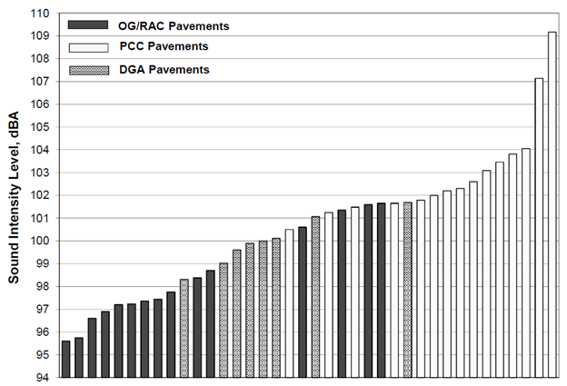
When selecting sites for model validation, consider the condition of the pavement for the road in question. In a validation model run, a pavement type is selected from FHWA TNM’s choices of dense-graded asphalt concrete (DGAC), open-graded asphalt concrete (OGAC), Portland cement concrete (PCC), or “Average” (derived from a combination of sound level data for dense-graded asphalt and Portland cement concrete). The vehicle reference energy emission levels in FHWA TNM were collected on several pavements that were neither new nor old or distressed. As such, choose model validation sites to avoid new or old pavements, which could lead to incorrect validation conclusions.
In any case, identify the pavement type at the validation site for use in the FHWA TNM model of the site. As shown in Figure 4-1, tire/pavement noise--based on on-board sound intensity (OBSI) measurements--varies considerably, even for the same type of pavement.[21] Note that FHWA requires the use of the “Average” pavement type in FHWA TNM for future sound level predictions unless express permission has been received from FHWA to use another pavement type. The OBSI level for TNM Average pavement would be approximately 102 dB to 103 dB.
Study objectives will often determine microphone locations. In choosing locations, be cognizant of localized noise sources that would affect or contaminate the measured levels, such as air conditioners, playing children, and dogs.
Model validation requires exercising care when taking measurements. While “existing level” noise measurements at residences are typically taken at an area of frequent human use that might be near a building like a house (e.g., a patio or the yard of a home), locate validation sites away from hard sound-reflecting surfaces such as building walls, retaining walls, solid fences, and signboards.[22]
ANSI/ASA S12.9-2013/Part 3[23] indicates that if the microphone is located within 25 ft (7.5 m) of a surface where reflections may influence the measured levels, then it should be positioned either flush against the reflecting surface or 3.3 ft to 6.6 ft (1 m to 2 m) away from the surface. In either case, an adjustment is then made to the measured sound level to approximate the level in the free field without the reflected noise contribution. ANSI/ASA S12.9-2013/Part 3 uses a -6 dB adjustment for the flush position and -3 dB for the 3.3 ft to 6.6 ft (1 m to 2 m) position.
American Society of Testing and Materials (ASTM) E966-10e1, which is the basis for the building noise reduction procedure in Section 6.0, relaxes these theoretical -6 dB and -3 dB adjustments to -5 dB and -2 dB respectively.[24] This handbook recommends these -5 dB and -2 dB adjustments for model validation measurements in the presence of reflected traffic noise.
In general, use a microphone height of 5 ft (1.5 m) above ground for validation measurements. However, receptors of interest may be at other heights above ground, such as outdoor balconies of multistory apartments or decks of single-family homes. If conditions are such that model validation measurements need to be made at these latter locations, then consider locating the microphone at the needed height on a tall mast 25 ft (7.5 m) or more away from vertical reflecting surfaces or at the above-noted close-in positions.
The one-hour A-weighted equivalent sound level [Leq(h)] descriptor is required when validating the FHWA TNM per 23 CFR 772.
For model validation measurements, the key instrumentation and accessories include the following:
Appendix B provides information and a discussion on instrumentation and other useful accessories and field supplies.
Consider three factors when selecting a sampling period:
The goal of these measurements is to validate the FHWA TNM model for the existing condition. Validation measurements do not need to be made during the worst noise hour and should not be done during the peak traffic hours if traffic flow is congested because FHWA TNM was not designed to predict sound levels for this condition.
However, knowing the existing worst hour is important for predicting the existing Leq(h) during that hour for comparison to the predicted future worst noise hour Leq(h) in the impact determination process, once the model has been validated. Consider making a 12-hour to 14-hour measurement at one or more representative locations along the project corridor to help identify the existing worst noise hour along the existing roadway. A typical time period could be 6 a.m. to 7 p.m. Collect the data in one-minute increments for easier identification of unrepresentative events for deletion from the data; then, combine the remaining minutes’ Leq to get the Leq(h) for each hour. Safely secure the sound level analyzer if it is being left unattended, perhaps by choosing a secure location in a fenced residential yard or by chaining the locked analyzer case to a tree, fence post or other fixed object.
An alternative technique for identifying the existing worst hour is to predict a series of daytime Leq(h) if hourly vehicle classification count data are available. In any case, do not assume that the worst noise hour for existing condition is the same as that for the future “build” condition.
Meteorological conditions can have a significant effect on measured sound levels and model validation. Avoid sound level measurements during precipitation or when the pavement is wet. Tire noise increases on wet pavements, especially in the higher frequencies that most affect an A-weighted sound level. In ideal circumstances take validation measurements under calm wind conditions on overcast days to minimize refraction effects that affect the measured sound level. The propagation algorithms in FHWA TNM assume a calm/neutral atmosphere (no wind and no change in temperature with height).
The change in wind speed with elevation above ground (“wind shear”) causes refraction of propagating sound waves: levels downwind from a source are higher than levels from the same source without wind, while levels upwind from a source are lower than levels without wind. These effects typically increase in magnitude with increasing distance from the source. Even close to the road, wind can flutter the microphone diaphragm and produce false noise readings (even through a proper windscreen). Do not make sound level measurements when winds exceed 11 mph (17 kmh or 5 m/s), regardless of direction (or delete any data collected during such periods during data analysis). If the A-weighted sound levels are lower than 40 dBA, even lower-speed winds can cause false noises.
The change in temperature with height above the ground (“temperature lapse rate”) can also have a major effect on measured sound levels by refraction. Except for briefly around sunrise and sunset, there will be a change in temperature with height, even on calm days. Compared to the neutral condition, levels for the same traffic volume, speed, and vehicle mix would be higher on clear nights during inversions (temperature increases with increasing height above ground) and lower during bright, sunny days (temperature decreases with increasing height above ground more rapidly than on calm, cloudy days).
Research presented in NCHRP Report 791[27] provides results for modeled meteorological conditions relative to calm and neutral atmospheric conditions. The research ran test scenarios with the SoundPLAN[28] computer program, using the Nord2000[29] sound propagation model, which accounts for detailed meteorological effects.[30]
Table 4-1 through Table 4-4 present some of the results from NCHRP Report 791. These tables detail differences in sound levels for: 1) upwind or downwind conditions for the neutral condition (no temperature gradient); and 2) temperature gradients for calm wind conditions. These data do not represent what might happen for combined non-calm and non-neutral conditions. The results are for a mix of automobiles and trucks for hard-ground and soft-ground sites with no noise barrier and for receiver heights above ground of 5 ft and 15 ft (1.5 m and 4.6 m) and receiver distances from the road of 50 ft to 1,600 ft (15.2 m to 488 m). Positive numbers in the tables indicate that sound levels are greater than the sounds levels with calm or neutral conditions, and negative numbers mean that sound levels are lower than those with calm or neutral conditions.
NCHRP Report 791 notes that “TNM users are encouraged to use the data in these tables to explain the difference in sound levels for validation purposes and for explanation of sound levels for agency and public purposes.” However, do not use the data in these tables or in the other tables in NCHRP Report 791 to adjust measured levels to validate or calibrate an FHWA TNM model run.
Table 4-1 note: 2.5 m/s = 5.6 mph; 5 m/s = 11.2 mph.
Table 4-2 note: 2.5 m/s = 5.6 mph; 5 m/s = 11.2 mph.
Cloud cover observations may be useful in assessing the potential for temperature refraction effects. Table 4-5 shows cloud cover classes. Class 1 has the least likelihood of temperature refraction, being closer to neutral temperature profile than other conditions. Class 4 has the greatest chance of refraction that could cause the largest decreases in level compared to neutral conditions, while Class 5 has the greatest chance of refraction that could cause the largest increases in level compared to neutral conditions. Avoiding measurements before sunrise or after sunset will typically bypass inversion periods. Measurement of temperature at two heights above ground, such as 5 ft and 15 ft (1.5 m and 4.6 m), is a precise way to determine lapse rate and the presence of refraction, but is not required for sound level measurements made for the purposes of the model validation called for in 23 CFR 772.
In choosing a measurement duration, a key consideration is to be able to represent the one-hour Leq with a shorter-term measurement to reduce time and cost for the measurement study, but without sacrificing accuracy. Measurement duration depends on how much the sound level fluctuates. Section 3.4.2 provides a discussion of guidance in ANSI/ASA S1.13-2005 (R2010) on classifying the temporal characteristics of environmental sound.
Please note that several unusually loud vehicles during a measurement near a lightly traveled road can skew the results of a shorter-duration measurement. On the other hand, along busier roads, loud vehicles should not, in general, be viewed as unrepresentative; they are part of the overall vehicle population, which includes a wide range of vehicle noise emission levels.
One guide for choosing duration is the greatest anticipated or observed range in the minimum and maximum sound levels occurring at the measurement site during the worst noise hour:
Additionally, most integrating sound level meters allow observation of the cumulative Leq during a measurement, even if the data are being accumulated in 1-minute intervals. If the cumulative Leq fluctuations do not settle down after measuring for the above durations, consider extending the sample period.
As noted in Section 3.0, a single sound level measurement at a site, regardless of its duration, only offers a slice or snapshot of the time-varying sound level at the site. Changes in traffic and in meteorological conditions, especially wind direction and temperature lapse rate around sunrise and sunset can change sound levels, sometimes substantially, as described earlier. However, for the purposes of model validation, a single sound level measurement at a site should be sufficient if concerns about other noise sources, meteorological conditions, traffic congestion, and unusually loud vehicles on low-volume roads have been addressed. Also consider:
This section presents the measurement procedure. More specific details for the person going into the field are in the FHWA Noise Measurement Field Guide. Prior to traveling to conduct the sound level measurements, plan the measurement study as described in Section 2.0.
The steps below describe what needs to be done upon arrival at the site, on through the successful collection of data.
For FHWA TNM, vehicles are grouped into five acoustically significant types (i.e., vehicles within each type exhibit statistically similar acoustical characteristics). These vehicle types are defined as follows:
Make classification counts (i.e., by vehicle type) by direction, ideally for the same interval duration as the sound level meter (e.g., one-minute), in case sound level data needs to be edited out.
Documentation is an essential part of every measurement. There are two stages to documentation: 1) in the field; and 2) after data analysis. This section describes field documentation. Field data sheets and more specific guidance are in the FHWA Noise Measurement Field Guide. Complete data sheets in the field while at the site. Make documentation sufficient for another person to return to that same microphone location and repeat the measurement with the same equipment and settings and under the same conditions. Here are some parameters to document using data sheets:
Typical data analysis and reporting procedures include these steps:
If the total measured level exceeds the background level by between 5 and 10 dB, then adjust the measured level for background noise to obtain the source-only level as follows:
![Ladj equals 10 times the log base 10 of [10 to the power of 0.1 times l sub c minus 10 to the power of 0.1 times l sub b] in dB.](image006.png)
 = 54.3 dB
Projects with multimodal noise sources (e.g., sources near a train line or airport) may require determination of train and aircraft noise levels to help establish the existing sound environment, predict the future sound environment, and evaluate noise abatement feasibility and mitigation design. Methods for undertaking this determination process are provided in this section, with additional information provided in Appendix E and Appendix F. Some of the information in this section is based on the 1982 FHWA document, Advanced Prediction and Abatement of Highway Traffic Noise.[31] This section updates the relevant and valuable procedures contained in the 1982 document. Updates include discussion of modern noise sources, methods, and available operational information.
Here are the types of projects to which the method applies:
The first few subsections discuss how to determine noise levels from other transportation noise sources. The remaining subsections discuss methods/applications for including these sources in highway traffic noise analyses. There are five methods/applications discussed:
The noise emanating from train and aircraft operations can contribute to the sound environment in a highway project area. The following subsections describe each of the noise sources and methods for determining the associated sound levels.
There are many similarities between train operations on railroad lines and highway operations. In both cases, operations occur on fixed paths, individual vehicles move past an observation point at a relatively constant speed, and there are a limited number of vehicle types with relatively similar spectral content for each type. Differences between train and highway operations relate primarily to the noise emission levels of individual vehicles and the time pattern of the operations. For train operations, there are fewer vehicles in each time period. Operations for light rail and commuter rail have set schedules for weekdays and weekends that are mostly consistent monthly. Freight rail operations can vary on a daily, monthly, and annual basis. Noise from train operations involves many parameters, including: type of train (light rail, commuter rail, freight); travel speed; number of locomotives and cars per train; number of trains per day; use of horns; use of train warning bells/chimes; use of crossing bells; and effects of special trackwork (e.g., turnouts and crossovers). Determining train noise levels to incorporate into highway analyses can be accomplished using screening estimates, measurements, or predictions, as described below.
Train noise can contribute to overall noise levels in a highway project area if associated noise levels are within 10 dB of highway noise levels. Practitioners can apply a quick-screening method to determine if this condition is the case, and if so, further evaluate train noise using measurements and/or predictions.
Applying the General Assessment Method in the Federal Transit Administration Transit Noise and Vibration Impact Assessment guidance manual[32] (section on estimating existing noise exposure) helps practitioners roughly estimate existing train noise in a project area. Table 5-1 shows estimates for train noise based on an average train traffic volume of 5 to 10 trains per day at 30 to 40 mph (48 to 64 kmh) for main line railroad corridors (does not include light rail). Noise levels are provided in terms of Day-Night Average Sound Level only (DNL, Ldn; 24-hour average level with nighttime penalty, see Appendix A for definition) and are listed for ranges of distances from the train noise source to a receiver. Distances are referenced from the track centerline, or in the case of multiple tracks, to the centerline of the rail corridor.
Table 5-1 notes: 1 ft = 0.3048 m. Sound levels do not include shielding from intervening rows of buildings. General rule for estimating shielding attenuation in populated areas: Assume one row of buildings every 100 ft (0.2 m); -4.5 dB for the first row, -1.5 dB for every subsequent row up to a maximum of -10 dB attenuation. (Extracted from Table 5-7 in the 2006 FTA guidance)
It is possible to measure existing train noise as part of highway noise project measurements near noise receptors of interest. If long-term measurements are being made to establish diurnal highway traffic noise patterns, then choose a measurement location such that the measured noise also captures train operations. Conduct these measurements similarly to those described in Section 3.0, following guidance to measure existing noise levels. Capturing at least 24 hours of data, establish existing noise that includes the train noise for where receptors in the highway project area are exposed to both sources. This would likely not apply to freight trains, since their operations can be highly variable. Consider the following when conducting such measurements:
If predictions will be made for existing or future conditions, then train source sound levels could be measured and used as input to the calculations (this could apply to any train type, including freight). Measure the maximum train noise level or sound exposure level (see definitions in Appendix A) and document the distance to the near tracks. Ideally, 10 pass-by events for each train type are used to calculate a representative average level. This is not a requirement for predictions; typical train noise levels are provided in FTA’s Transit Noise and Vibration Impact Assessment guidance manual.[33] FTA guidance also provides measurement guidance specific to trains. Using FTA or Federal Railroad Administration (FRA) methods, calculate the DNL or the worst hour sound level using either measured or listed train noise levels.
To predict train noise levels, use a simplified manual method, FTA’s General Assessment Method (also in FRA CREATE prediction spreadsheet), FTA Detailed Analysis Method, or the HUD quick method (described in Section 5.1.1.3.3). There are also commercial software packages to predict train noise, but these are not discussed in this document.
A simplified manual method can be used to calculate rail noise. This method is based on FTA and FRA general assessment techniques and is shown in Appendix E. The calculation method requires input about the trains, tracks, and operations. The simplified method includes freight, commuter, and light rail. The resulting rail noise predictions are provided for both the peak hour Leq and the DNL.
FTA’s guidance document provides both general assessment and detailed analysis techniques for predicting rail noise. The simplified manual method described previously is based on the General Assessment Method; the simplified method can be further refined using the additional noise sources found in FTA’s guidance document and executed in the FRA CREATE model.[34] In addition, the Detailed Analysis Method in FTA’s guidance document can be applied for a more comprehensive assessment of rail noise. This method requires additional input parameters such as terrain geometry, ground type, additional track parameters, specific stationary source parameters, and noise barrier parameters. FTA’s Detailed Analysis Method permits the most accurate prediction of train noise compared to other methods described in this document.
The HUD quick method (DNL Calculator[35]) permits online calculation of train noise. This method requires knowledge of train types and operations; however, assumptions are provided in the HUD Noise Guidebook[36] for when some of the parameters are not known. Listed below are assumptions that can be made for an estimate:
There are major differences between aircraft and highway operations. For aircraft, there are relatively few noise events, but those that do occur can have high noise levels. The pattern of operations is irregular throughout the day and can vary on a daily or monthly basis. Noise from aircraft operations in flight and at an airport involves many parameters, including: type and weight of aircraft; number of arrivals and departures, and types of procedures; flight paths; and aircraft run-ups and other ground operations. To determine aircraft noise levels to incorporate into highway analyses, use published noise contours, measurements (likely could not capture representative noise during highway noise measurements), or predictions, as described in the following sections.
Find estimates of aircraft noise in a highway project area in published airport noise contours. For many civil, military, and general aviation airports, noise exposure contours are already available from local government or airport authorities. These are often generated as part of an airport master plan, airport expansion, or environmental assessment study. An internet search can provide a noise practitioner with such contours. Noise levels can be extracted by locating a highway project area on the contour map and extracting the appropriate DNL. Airport contours usually show levels down to a DNL of 65 dBA, and there could be lower levels that contribute to the noise in a highway project area. Further investigation may reveal lower-level contours (various reports for airport noise studies), and lower-level values can be extracted from those. An alternative is to apply prediction methodologies to reveal levels/contours below a DNL of 65 dBA.
It is possible to measure existing aircraft noise as part of highway noise project measurements near noise receptors of interest. If long-term measurements are being made to establish diurnal highway traffic noise patterns, then choose a measurement location such that the measured noise also captures aircraft operations. Conduct these measurements similarly to those described in Section 3.0, following guidance to measure existing noise levels. Capturing at least 24 hours of data, measure existing noise that includes the aircraft noise for where receptors in the highway project area are exposed to both sources. However, these data would likely not be representative of average aircraft noise, since their operations and the weather can be highly variable. Consider the following when conducting such measurements:
Aircraft noise levels can be predicted using the Federal Aviation Administration (FAA) method. There are also commercial software packages to predict aircraft noise; these are not discussed in this document. Simplified manual methods for predicting aircraft noise were previously documented by FHWA, the Environmental Protection Agency (EPA), and HUD; however, while the methods are valid, the published source sound levels are outdated. Current aircraft source sound levels are included in the FAA aircraft noise prediction software in the required metric but are not easily translatable for use in a simplified manual method. Practitioners can use FAA’s model, Aviation Environmental Design Tool (AEDT) to develop predictions.[39] Input to the model includes operations by aircraft type and time of day. Some operational information is available on FAA’s website, and practitioners can contact local FAA or airports to supplement the information.[40]
The following subsections describe circumstances for considering train and aircraft noise. As a first step, screen for possible contributions from train or aircraft noise using the train noise screening method in Section 5.1.1.1 and aircraft contours (Section 5.1.2.1). If existing or future noise levels (alone or combined, per Equation 5-1 in Section 5.2.1) are within 10 dB of anticipated highway noise levels, then consider train or aircraft noise sources further as described in the following subsections.
For Type I highway construction projects, one criterion for assessing impacts is if there will be a substantial increase in traffic sound levels because of the project. To evaluate substantial increase, the predicted future sound levels need to be compared to existing noise. Consider transportation noise sources to determine existing noise near train or aircraft operations. Existing traffic noise levels can be measured at representative locations on a highway project, as described in Section 3.0. Train and aircraft noise can be measured as part of the existing noise measurements in the project area. However, the measurement period may not represent typical train or aircraft operations; please refer to Section 5.1.1.2 (trains) and Section 5.1.2.2 (aircraft) for more information. Also, the traffic noise measurement location may have been purposefully chosen to avoid these sources, although there may be receptors exposed to these sources. If it is not possible to measure all noise sources together, or if it is determined that the train or aircraft noise during the measurement period is not representative, then consider three steps:
For the combining noise sources, three primary metrics are considered: the worst noise hour [Leq(h)], the DNL (Ldn), and the Community Noise Equivalent Level (CNEL, Lden; DNL with an additional noise penalty for evening hours—see definition in Appendix A). Equation 5-1 represents combining levels for all three of the listed metrics, assuming the metrics are the same for the three modes of transportation (if only two modes are being considered, then eliminate the term for the third mode).
Equation 5-1: Calculation of Combined Sound Levels

where:
Lcombined is the combined noise level [applying the Leq(h), Ldn, or Lden metric];
Lhighway is the highway noise level;
Ltrain is the train noise level; and
Lair is the aircraft noise level.
Depending on how train noise is determined, the resulting metric is either Leq(h) or DNL. For the Leq(h) metric, the highway noise and train noise can be directly combined. For the DNL metric, highway noise will first need to be converted to DNL before combining with the train noise [please refer to Appendix F on how to convert highway Leq(h) to DNL].
Aircraft noise is usually presented using the DNL metric. To combine with highway noise, highway noise will first need to be converted to DNL before combining with aircraft noise [please refer to Appendix F on how to convert highway Leq(h) to DNL].
Highway projects require determination of the worst noise hour for existing conditions. This is accomplished via measurements or modeling (the latter applicable only to an existing highway with use of a validated model). For measurements, identify worst hour by conducting long-term measurements. Train and aircraft noise could influence determination of the worst noise hour, particularly when microphones are placed near freight rail or other loud operations that can increase hourly noise levels. Consider train and aircraft operations in determining the worst hour. Refer to FHWA policy on when to include and exclude noise from other transportation sources for worst highway traffic noise hour determinations.
To include other transportation noise sources, ensure the train and/or aircraft operations are representative during the measurement period; refer to Section 5.1.1.2 for more guidance on this. To exclude other transportation noise sources, they would need to be eliminated before identifying the worst hour. If long-term measurements are attended or if audio is being recorded, then eliminate train and aircraft events from the time histories by identifying the events by logged time and time signature. If long-term measurements are unattended and if audio is not being recorded, then the events would need to be identified by time signature, which is not always reliable. Long-term measurements attended during suspected worst highway traffic noise hours (an hour before through an hour after peak commuting times, assuming no congestion) can facilitate positive event identification.
Measured existing highway traffic noise is compared to predicted existing highway traffic noise—using traffic classification counts and speed measurements made during the sound level measurement, as described in Section 4.0—to validate a FHWA TNM case constructed for a highway traffic noise project. Since FHWA TNM accounts only for highway traffic noise sources, it is necessary to eliminate other noise sources from the measured levels that would interfere with the validation. These include neighborhood noise sources (e.g., lawn mower, generator) and other transportation noise sources. When existing noise measurements are conducted, isolate and eliminate train and aircraft and other intrusive noise sources from the measured data before finalizing the representative noise level. This could be accomplished by pausing measurements during a contaminating noise event or logging the contamination time for later elimination. As an example, if a one-minute data block includes a train pass-by event, then eliminate that minute, and recalculate the short-term measurement Leq without that minute. Section 4.0 provides details.
If other noise sources need to be considered for future noise impact determinations, then add train and aircraft noise sources to the predicted highway traffic noise levels via the following method:
To determine highway noise impacts, assume DNL = Leq(h) + 2, described further in Appendix F. FHWA may provide further guidance on this assumption in the future.
Consider the type of impact analysis required. An FTA or FRA analysis may be required for a highway project that moves train tracks closer to a sensitive receptor. If this is the case, then existing noise—including the train—would need to be established at sensitive receptors; for residential receivers, this requires use of the DNL metric. Also, due to FTA/FRA requirements, consider using additional receptors. Concerning data collection, the LAFmx for trains may need to be measured for use in FTA or FRA models, or apply the published levels in FTA and FRA guidance, as described in Section 5.1.
It is necessary to consider all noise sources as part of noise abatement reasonableness for highway projects. Failure to account for other environmental noise may result in ineffective noise abatement. It is important to understand the sound level and source locations for each source, and whether abatement designed for the highway reduces the noise, when considering other transportation sources in the reasonableness analysis.
The following method considers other transportation noise sources in abatement analysis:
Highway noise abatement may be effective for train noise, depending on the location of the train tracks. In this case, both the highway and train noise would be reduced with a noise barrier, and the overall sound level combining the two noise sources would be reduced. If the barrier reduces only the highway noise, then the overall noise may not be reduced, depending on whether highway noise is the dominant source. Please refer to Table 5-2 for examples. The first example shows the predicted highway noise is 70 dBA without a barrier, the train noise is 70 dBA without a barrier, and the total noise is 73 dBA (please refer to Equation 5-1). If both highway noise and train noise are reduced 10 dB with the barrier, then each noise source becomes 60 dBA, and the combined noise is 63 dBA. However, if the train noise is not reduced by the barrier, then the total noise would be 70 dBA, as shown in the second example. The third example shows a train noise level lower than the highway noise level, but with the barrier having no effect, the total noise with the barrier in place is dominated by the train noise.
For aircraft noise, highway abatement barriers would likely not be effective to reduce in-flight aircraft noise. However, highway noise barriers may reduce noise from airport ground operations. The last example in Table 5-2 shows aircraft noise being unaffected by a highway noise barrier and how it becomes the dominant noise source with the noise barrier in place.
Note: Sound levels are in Leq(h) or DNL
Since highway noise is a mostly continuous noise source, focusing abatement on highway noise would help to reduce noise in communities most of the time. However, during train or aircraft events, the highway noise abatement may or may not have an effect.
One additional consideration is that highway noise barriers may reflect other noise sources back toward a receptor, increasing the noise from the other source. Consider a more appropriate barrier placement that may avoid such reflections.
This section describes recommended procedures for the measurement of:
The main use of this measurement procedure is on Type I highway project noise studies where a building-specific OINR or an interior noise level is needed for impact assessment. Also consider using this procedure in unusual specialized situations such as:
This section may be used for interior microphone placement if the goal is only to determine existing interior sound levels for the purposes of impact assessment per 23 CFR 772. Then follow the procedures in Section 3.0 for the rest of the measurement.
The following procedures are in accordance with ASTM E966-10e1.[41] The ASTM Standard Guide for Field Measurements of Airborne Sound Insulation of Building Facades and Facade Elements defines OINR as “the difference in sound pressure level between the free-field level outdoors in the absence of the structure and the resulting sound pressure level in a room.” In this procedure, measurements of the existing traffic noise are made simultaneously outside and inside the building. If traffic is not present as a noise source (e.g., a new alignment project), then a fixed loudspeaker system may be used as an artificial noise source. ASTM E966-10e1 further notes that if “the A-weighted noise reduction due to the actual source is reported, the result is called noise level reduction.” Acknowledging that note, the term OINR will be used in this handbook to distinguish it from other types of noise level reduction.
The OINR would typically be applied to an exterior sound level as predicted by FHWA TNM to determine an interior level for an Activity Category D land use. As described in the FHWA noise regulation in 23 CFR 772, Activity Category D includes certain land-use facilities (listed in Activity Category C) that may have interior uses, specifically: “auditoriums, day care centers, hospitals, libraries, medical facilities, places of worship, public meeting rooms, public or nonprofit institutional structures, radio studios, recording studios, schools, and television studios.” Interior Noise Abatement Criteria (NAC) are not included in 23 CFR 772 for residential land uses (Activity Category B), and hotels, motels, offices and restaurants/bars, and other developed lands. However, these procedures could also be used for these types of buildings if needed for some other purpose.
Further, 23 CFR 772.11(c)(2)(iv) states the following:
“A highway agency shall conduct an indoor analysis after a determination is made that exterior abatement measures will not be feasible and reasonable. An indoor analysis shall only be done after exhausting all outdoor analysis options. In situations where no exterior activities are to be affected by the traffic noise, or where the exterior activities are far from or physically shielded from the roadway in a manner that prevents an impact on exterior activities, the highway agency shall use Activity Category D as the basis of determining noise impacts.”
In addition, the FHWA Highway Traffic Noise: Analysis and Abatement Guidance states the following:
“In the absence of calculations or field measurements, compute interior noise level predictions by subtracting noise reduction factors from the predicted exterior levels for the building in question, using the information in Table 6 [of that document]. Noise analysts should take interior noise measurements for the final noise analysis and abatement design for locations where highway agencies consider noise insulation as an abatement measure.”[42]
Table 6-1 presents typical OINR from the Guidance document, which lists them as building noise reduction factors.
Table 6-1 notes: This table was derived from Table 6 of the Guidance document. Consider windows open unless there is firm knowledge that the windows are in fact kept closed almost every day of the year.
This table provides conservative results. The actual OINR depends on wall construction, façade surface area, percent of façade surface area for windows and doors, window opening area, roof and ceiling construction, window construction, etc. If some or all of these parameters are known or can be estimated, OINR calculations can be made using ISO 12354-3:2017, “Building acoustics - Estimation of acoustic performance of buildings from the performance of elements - Part 3: Airborne sound insulation against outdoor sound.” Follow-up with measurements should be made, where practical, to verify interior impacts if modeling predicts them.
Site selection for measurements is generally driven by study goals. In this case, the goal either is to determine an OINR or to determine interior noise levels (or both). Specifics may depend on the project sponsor’s noise policy or procedures.
There are two aspects to consider regarding site selection:
For the purposes of 23 CFR 772, the site should be one of the Activity Category D land uses listed above. Specifically, the site should be one where: 1) an exterior impact has been identified and exterior abatement measures (such as a noise barrier) will not be feasible and reasonable or 2) no exterior activities are to be affected by the traffic noise or where the exterior activities are far from or physically shielded from the roadway in a manner that prevents an impact on exterior activity areas.
Choose as the interior location(s) one or more rooms or spaces of interest such as school classrooms, worship spaces, medical examining rooms, and patient rooms that face the existing or proposed highway. Choose a room or space that is completely enclosed and stop all noise-generating activities in the room during the measurements. The interior background sound level needs to be at least 10 dB below the lowest anticipated maximum A-weighted sound pressure level (LAFmx) of vehicle pass-bys. If not, then the full measure of the OINR cannot be determined; instead only a lower bound to the OINR can be determined.
Look for an exterior measurement site with the following geometric characteristics, which may be difficult to find because a specific building in its unique surroundings is typically being tested:
A room volume less than 5,300 ft3 (150 m3)[43] necessitates only a single microphone position. Place the microphone at 5 ft (1.5 m) above the floor of the interior location and at least 3 ft (1 m) from any walls (Figure 6-1).
If the room volume is 5,300 ft3 (150 m3) or greater, use multiple fixed microphone positions. The largest dimension of the interior test wall facing the road should be divided by 10 (by 3 if in meters) and rounded to the next highest integer to determine the number of microphone positions.[44] These microphone positions should be 3.3 ft to 6.5 ft (1 m to 2 m) from the test wall and at least 3.3 ft (1 m) from all other walls, at a height of 4 ft to 5 ft (1.2 m to 1.5 m) above the floor.
There are four possible locations for the placement of the exterior microphone. Positions 1a, 2 and 3 are shown in Figure 6-1:
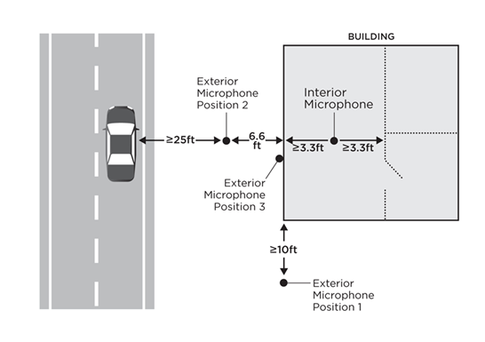
If a loudspeaker is used as the source, locate it at a distance from the building façade such that the ratio of the distances from the loudspeaker to the farthest (D1) and nearest (D2) parts of the façade covering the room to be tested (not the entire façade) is no greater than two (i.e., D1/D2 is less than or equal to 2). Calculate this distance beforehand to ensure that the measurement will be feasible. Also calculate this distance if the remote, calibrated loudspeaker approach (Position 1b) is going to be used. Angle the loudspeaker toward the façade at a preferred incidence angle of 45°[46] as shown in Figure 6-2. This angle, θ, is determined by the perpendicular to the façade at the midpoint of the room to be tested and the line joining the loudspeaker to the midpoint.
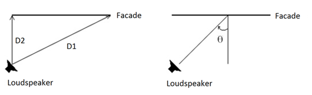
Use the equivalent sound level (Leq) for determining the OINR.
Since measurements are to be done simultaneously, two sets of equipment are needed.
Note that traffic data collection, while possibly of interest, is not required for this procedure because the goal is to determine the difference in the indoor and outdoor levels and the indoor and outdoor measurements are being done simultaneously.
Appendix B provides specifications for loudspeakers under the heading of “artificial noise source.” The signal needs may require a pre-study field review to conduct a measurement of the background one-third octave band sound pressure levels in the interior space to be tested (with interior noise sources quieted), followed by an estimation of the needed one-third octave band sound pressure levels at the exterior façade. This calculation could assume that the A-weighted OINR will be 10 dB for an open-window test and from 20–35 dB for a closed-window test, using Table 6-1 for guidance. See step six in Section 6.6 on how to use the measured one-third octave band sound pressure levels to compute an A-weighted OINR.
Consider three factors when selecting a sampling period:
The goal of these measurements is to determine the OINR for test rooms or chosen interior spaces. For traffic as the noise source, these measurements do not need to be made during the worst noise hour and should not be done when traffic flow is congested because the traffic noise level will be lowered, making it more difficult to determine the full amount of the OINR. Ideally, conduct measurements under a steady or fluctuating—yet continuous—flow of traffic. If traffic is intermittent (as discussed in Section 3.4.2), ASTM E966-10e1 recommends measurements of the Sound Exposure Level (SEL) of individual vehicle pass-bys instead of the time-averaged Leq because periods of no traffic would lower the Leq, making it more difficult to determine the full amount of the OINR. This handbook suggests another approach: measure Leq, but pause sampling during lulls in traffic. This alternative is much easier than trying to measure SELs by vehicle type and then constructing an OINR that is weighted by vehicle type.
For the loudspeaker as the noise source, measurements may be made at any time when the background sound level from other noise sources is 10 dB or more below the loudspeaker level outside the façade of the room being tested. Background noise is unlikely to be an issue because the loudspeaker level will have to be quite high to determine the full OINR.
Meteorological conditions are less important for these measurements than for other types of measurements because a noise reduction is being determined, not a level that will be used for impact determination or other purposes. However, do not conduct sound level measurements during precipitation or when the pavement is wet. Tire noise increases on wet pavements, especially in the higher frequencies that most affect an A-weighted sound level and therefore an A-weighted noise level reduction. Also, wind can flutter the microphone diaphragm (even through a proper windscreen), producing false noise reading. Do not make sound level measurements when winds exceed 11 mph (17 kmh or 5 m/s), regardless of direction (or delete any data collected during such periods during data analysis). If the A-weighted sound levels are lower than 40 dBA, even lower-speed winds can cause false noises.
Unlike some of the other measurement procedures in this handbook, the goal of these measurements is not to represent the one-hour Leq with a shorter-term measurement. A key consideration in choosing a measurement duration is the need to properly represent the spectrum of the traffic noise and accurately determine the A-weighted noise level reduction:
Also, for all the methods, use multiple fixed microphone positions if the room volume is 5,300 ft3 (150 m3) or greater, as described in Section 6.1.2.1. Simultaneously using more than one interior sound level measurement system could expedite the data collection process.
Repeating the measurement more than once can help address any variability in the result. As noted, the goal of this procedure is to determine a difference in levels—the OINR—not to determine a representative Leq(h) and thus there should be less variation in the result.
For continuous traffic and the loudspeaker method, perform a quick field calculation of the OINR after the first measurement by subtracting the interior Leq from the exterior Leq. If multiple interior measurement positions are used, then calculate and average each OINR. Then, repeat the measurement and calculate this second measurement’s OINR or average OINR.
Make a third measurement if the OINR for the two measurements differs by more than 3 dB. If none of the three measured OINR are within 3 dB of each other, then identify the cause of the variation, and repeat the measurement after the cause has been identified and rectified. For intermittent traffic, it may not be feasible to repeat the measurement if the traffic volume is low.
This section presents the measurement procedure. More specific details for the persons going into the field are in the FHWA Noise Measurement Field Guide. Prior to traveling to conduct the sound level measurements, plan the measurement study as described in Section 2.0. Choose the noise source (traffic or loudspeaker), including how to power the loudspeaker system, if used. Also, determine the microphone positions. Having at least one person outside and one person inside the test room is important for assuring validity of the collected data. Coordinate with the building owner or manager and the occupants during a pre-measurement field review and at the time of the measurement.
Perform the following steps for any of the exterior microphone positions. For Position 1a (the calibrated loudspeaker approach), perform the relevant steps at the remote site first, prior to the set up and measurements at the study site.
If traffic flow is continuous, then the background level cannot be determined and the operator must judge if any background noise sources that are present are causing an increase in the total measured level. Audibility of the background noise source is an important evaluation factor. If not audible, then the background noise is likely not affecting the total level and no background adjustment is needed. If audible, then determine an upper limit to the background level by measuring the L90 statistical descriptor. Report such upper-limit background levels as “assumed.” (Most integrating sound level analyzers have the built-in capability to measure statistical descriptors and can be set to measure L90.)
Documentation is an essential part of every measurement. There are two stages to documentation: 1) in the field; and 2) after data analysis. This section describes field documentation. Field data sheets and more specific guidance are in the FHWA Noise Measurement Field Guide. Complete data sheets in the field while at the site. Make documentation sufficient for another person to return to that same microphone location and repeat the measurement with the same equipment and settings and under the same conditions. Here are some parameters to document using data sheets:
Typical data analysis and reporting procedures include the following steps:
If the total measured level exceeds the background level by between 5 and 10 dB, then adjust the measured level for background noise to get the source-only level as follows:
Equation 6-2: Formula for Adjusting Leq for Background
where: Ladj is the background-adjusted measured level;
Lc is the total measured level with source and background combined; and
Lb is the background level alone.
For example, if:
Lc = 55.0 dB
Lb = 47.0 dB
Then:
Equation 6-3: Example of Background Adjustment
 = 54.3 dB
Lexterior is the exterior level, adjusted as needed; and
Linterior is the exterior level, adjusted as needed.
For exterior microphone at Position 1a or 1b:
OINR = Lexterior - Linterior (dB).
For exterior microphone at Position 2 located near the facade, account for the sound pressure increase with a -2 dB adjustment:
OINR = Lexterior - Linterior - 2 (dB).
For example, if:
Lexterior= 77.0 dB
Linterior= 50.0 dB
Then:
OINR = 77.0 – 50.0 - 2 = 25 dB
For exterior microphone at Position 3 flush with the facade, account for the sound pressure increase with a -5 dB adjustment:
OINR = Lexterior - Linterior - 5 (dB)
For example, if:
Lexterior = 80.0 dB
Linterior = 50.0 dB
Then:
OINR = 80.0 – 50.0 - 5 = 25 dB
This section describes recommended procedures for performing existing groundborne vibration measurements near highways. There are no Federal requirements regarding traffic-induced vibration. Vibration measurements may be conducted for two reasons:
Vibration data may be collected for:
Knowing the existing level of vibration may be important for multimodal projects, particularly those where nearby railroad tracks are relocated. Additional analysis may be required by FRA or FTA when tracks are relocated or train schedules are significantly changed.
Groundborne vibration is measured by transducers that measure the vertical motion of the ground or surface to which they are attached. There are two commonly used types of transducers used for measuring groundborne vibration. Geophones, which measure vibration velocity, and accelerometers, which measure vibration acceleration. Both types of device are acceptable for use in measuring, though accelerometers must have their signal converted to vibration velocity, either through an electrical integrator in the data recording system, or in post processing. “Transducer” will be used here to refer to either a geophone or an accelerometer. Further information about transducers is included in Appendix B.
In addition to vibration, groundborne noise may be of concern. Groundborne noise is the sound produced from floors and walls shaking due to groundborne vibration. This noise typically has a low frequency rumbling characteristic. Groundborne noise may occur in conjunction with airborne noise; however, at most receptors airborne noise will be the dominant source. Some exceptions include buildings with no windows or doors facing traffic, or receptors behind existing noise barriers. In these cases, groundborne noise may be the dominant noise source.
Groundborne noise is difficult to measure directly. Sound may be measured in an interior space, but it is often difficult to distinguish between the airborne contribution and the groundborne contribution. It may be possible to measure noise in an interior space and derive the groundborne noise in buildings where the reduction from outdoor-to-indoor noise is known (Section 6.0). Similarly, it can be assumed that direct measurement of sound levels will correlate with groundborne noise in interior spaces where the penetration of noise from the exterior is low.
Typically, groundborne noise is indirectly calculated from the measured groundborne vibration. To derive groundborne noise, an assumed radiation factor (Krad) is added to the measured vibration. Section 7.2 suggests Krad assumptions. Groundborne noise is also predicted using an A-weighting adjustment. Therefore, it is necessary to collect vibration data in one-third octave bands so that the A-weighting may be applied during post processing.
Consider conducting background noise measurements in special cases where ambient noise inside a receiver is low, such as a recording studio or concert hall. This would require a low-noise microphone and recorder system. Knowing the existing noise levels inside these spaces can be useful for comparison to any predicted groundborne noise levels. This section only discusses vibration measurements and does not address low-noise interior measurements.
Site selection is guided by the location of vibration-sensitive receptors. Vibration-sensitive receptors include residences, offices, schools, and churches. Additionally, receptors such as hospitals or research laboratories may house equipment that is sensitive to vibration. Please refer to FTA’s guidance in Transit Noise and Vibration Impact Assessment for additional examples of groundborne vibration-sensitive uses.[48]
Site selection is guided by the location of vibration-sensitive receptors and major nearby vibration sources. Vibration-sensitive receptors will mostly mirror noise-sensitive receptors. The same techniques used to identify potential NSAs can be used to identify vibration-sensitive areas (Section 3.1.1). Potential vibration-sensitive areas can be identified using land-use maps, aerial photos (including web-based mapping sites), and field reconnaissance. The vibration measurement study should include residential areas. When selecting sites, consider the representativeness of the site.
For groundborne noise, consider the topography and building construction. Consider conducting measurements at receptors where groundborne noise is expected to dominate airborne noise. This includes receptors where the airborne sound path is blocked, such as areas behind noise barriers. Additionally, there may be land uses that are sensitive to vibration, but not to noise. These types of land use typically house vibration-sensitive equipment, and may include vibration-sensitive manufacturing, hospitals, and university research operations. High-power electron microscopes can be sensitive to vibration, and even optical microscopes may be difficult to use when vibration is below human annoyance levels. Highway operations do not usually affect vibration-sensitive equipment, but it is possible for highway construction to interfere with use of such equipment.
Site selection should also consider roadway irregularities. Discontinuities in paving—including potholes, changes in pavement type, and bridge expansion joints—can add significantly to the vibration levels. Some discontinuities, such as joints, should be considered permanent features in the roadway, while features like potholes are not. Whether to measure near discontinuities is dependent on the type of project, and it can be left to the practitioner’s judgment.
Study objectives will usually dictate transducer locations. Measurements at residences are usually taken at or near the building. Avoid extreme locations—either too close to the road or too far from it—in order to accurately capture vibration impacts. In choosing locations, be aware of localized vibration sources that would affect or contaminate the measured levels, such as air conditioners, children, and dogs. Consistency in sensor locations is desirable, with site conditions possibly dictating deviations.
FTA offers guidance about placement of transducers indoors or outdoors: “Although groundborne vibration is almost exclusively a problem inside buildings, measurements of existing ambient vibration should generally be performed outdoors.”[49] Some exceptions to this guidance are suggested such as when “equipment and activities inside the building …cause greater vibration than that due to external sources.”
Firmly affix the transducer to the ground. If the chosen site has smoothly paved surfaces, then epoxy, museum wax, or earthquake gel may be used to mount the transducer. Attach sensors in soil to a spike or stake inserted into the ground. The geological conditions near the site should be considered, including large visible rocks, bodies of water, and any significant changes in the ground level. The type of surface to which the transducer will be fixed should be reasonably representative of the nearby geology. The transducer should be firmly attached to the ground below it. Soft top-layers should be avoided, such as loose gardening soil, mulch or leaves, or gravel.
Interior vibration may also be measured in cases such as when sensitive equipment is located within the receptor, or when it is necessary to document already high vibration levels from internal operations. A vibration transducer should be placed at the center of the floor span where the amplitudes are highest. The transducer should be firmly affixed to the floor. On floors with hard surfaces, transducers may be adhered similarly to exterior positions. Removeable adherents such as museum wax or earthquake gel are preferred for indoor positions. For carpeted areas, the transducer should be affixed to the hard floor below the carpet. The transducer should be mounted on a plate or block with three leveling nails or spikes. The spikes must penetrate the pile of the carpet and the carpet pad and contact the hard surface below. The system must have sufficient weight to hold the transducer in good contact with the floor through the spikes. This may be achieved either by using a heavy metal plate or by adding weight with sand bags or similar weights. For thin carpeting mat, the use of nails or spikes can be eliminated, but weight should still be added to the plate or block.
Groundborne vibration and noise use similar descriptors to airborne noise. Additionally, the groundborne vibration is directly related to the groundborne noise.
Groundborne vibration is characterized by the vertical vibration velocity. It is typically sufficient to measure only the vertical component. According to FTA, “Although transverse components can submit significant vibration energy into a building, the vertical component usually has greater amplitudes than transverse vibration.”
The root-mean-square (RMS) levels of groundborne vibration characterize human response, while peak particle velocity (PPV) levels of groundborne vibration characterize the potential for building damage. Vibration is reported in decibels, referenced to 1x10⁻⁶ in/sec, and designated VdB. Groundborne vibration does not include any weighting. The RMS averaging time or time constant should be one second.
The ambient vibration is characterized by the Leq for some desired period. Unlike for noise (Section 3.2) it is not required to specifically identify the 1-hour Leq. The appropriate measurement duration is discussed in Section 7.4, and will depend on the project. Statistical descriptors (e.g., L90) may also be used to further understand the vibration environment.
The RMS level for the duration of the event is typically used when characterizing a single event, such as a vehicle pass-by. The maximum RMS level (Lmax) may also be used, as it may be easier to obtain than the average level for an event. Groundborne vibration RMS levels may be collected in one-third octave bands. FTA defines its detailed vibration criteria levels in terms of one-third octave bands. Recording spectral data is necessary for conversion to groundborne noise, discussed in Section 7.2.2.
The same descriptors used for groundborne vibration may be used for groundborne noise. However, the groundborne noise must be presented in terms of sound pressure level and include A-weighting. Therefore, groundborne noise is reported in dBA. The A-weighted equivalent sound level (Leq) for the measurement period should be used to characterize ambient noise level. Statistical descriptors (e.g., L90) may also be used to further understand the groundborne noise environment. Single events may be characterized by the average RMS level for an event or by Lmax level for an event. Groundborne vibration and groundborne noise are intrinsically connected, so the same descriptor should be used for both.
Predicted groundborne noise is often derived from the measurement of groundborne vibration. The noise is calculated by
Equation 7-1: Derivation of Groundborne Noise
LA = LV + Kawt + Krad (dB)
where: LA is the A-weighted groundborne noise level, in dBA;
LV is the measured groundborne vibration level, in VdB;
Kawt is the A-weighting (Table 17-1 shows A-weight values by one-third octave band); and
Krad is the radiation factor.
The current FTA-recommended Krad is +0 dB[50] and the FRA-recommended Krad is -5 dB. These values for Krad are suggestions for typical buildings. Spaces that have large, flexible surfaces may have much higher groundborne noise levels, as high as +10 dB. These spaces can include halls, performance spaces, or gymnasiums. FTA’s Transit Noise and Vibration Impact Assessment[51] and the FRA High-Speed Ground Transportation Noise and Vibration Impact Assessment[52] include further discussion of Krad. Groundborne noise is similarly calculated, whether LV represents an ambient level (Leq) or an event maximum RMS level (Lmax).
See Appendix B for discussion of and information on instrumentation. Two types of transducers are recommended—accelerometers and geophones. Only one type needs be deployed for a measurement. Geophones measure ground velocity directly, while accelerometers measure ground acceleration. If an accelerometer is used, then the data will need to be integrated to obtain vibration velocity. This may be done at the recorder level or completed in postprocessing.
Needed instrumentation for vibration measurements include the following:
Some sound level meters can record input from transducers other than microphones, including accelerometers or geophones. Take care to ensure that vibration velocity is measured with a flat weighting if using a sound level meter. No A-weighting should be applied to vibration measurements, and the signal should be integrated to velocity if using an accelerometer. The frequency bandwidth for vibration should include frequencies as low as 1 Hertz (Hz). Meteorological data is not generally required for groundborne vibration measurements.
As noted, consider interior noise measurements in some specialized cases. These measurements require a low-noise microphone and data recording system. No additional discussion of low-noise measurements is included here.
The sampling periods for groundborne vibration mostly carry the same considerations as for airborne noise (Section 3.4). For vibration, weather is not generally considered, though measurements should be avoided if there is heavy rainfall. Consider three factors when selecting a sampling period:
Exterior vibration measurements may be made for two reasons:
The ambient vibration is characterized in terms of Leq for some continuous period. The duration of this period is discussed in Section 7.4.2, and may range from 10 to 30 minutes. Specific events, such as vehicle pass-bys, are characterized using the maximum RMS level (Lmax) during the time that the vehicle passes by. The RMS should be averaged using a time constant of one second.
The appropriate time to conduct exterior existing vibration measurements will depend on the information sought. If ambient vibration is sought, then the measurement can be conducted as is for measuring existing noise (Section 3.4.1 and Section 4.4.1). The highest period of groundborne vibration does not necessarily correlate with the highest hour of noise. The highest vibration can depend on traffic volume, speed, vehicle makeup, and the presence of irregularities in the road. The vehicle makeup should be documented when traffic is a major contributor to the measured vibration levels.
If characterization of specific events is desired, then the period to measure should coincide with when those events are likely to occur. Measurement of bridge joints or other roadway irregularities should take place when traffic is moving at maximum flow and when there are a variety of vehicle types. Railway schedules should be consulted and measurements conducted when nearby trains are operating.
Although not common, there are some cases where measurements of indoor vibration are important. Possible reasons to conduct vibration measurements at a building interior include the following:
At these locations, the use of the space will inform the optimal period for measurement. For example, at a radio or television recording studio, there may be operations early or late at night. There could be little traffic, rail, or other activities while the studios are in use. Background vibration inside the studio should be measured during a period that reflects these low ambient conditions. Interior measurements documenting low ambient conditions should be made in unoccupied spaces.
Groundborne vibration is not highly sensitive to meteorological conditions. However, vibration is sensitive to the conditions of the ground. Falling rain or hard precipitation can cause excess vibration at the sensor and mask the typical ambient or traffic vibration. Frozen ground and unusually saturated or dry ground can also affect the propagation of vibration. Vibration measurements should be made during typical conditions for the local area.
Two considerations should be balanced when choosing a measurement duration. The first consideration is the ability of the measurement period to represent a one-hour vibration Leq. The second consideration is the ability of the measurement period to capture any relevant high-vibration events. Section 3.4.2 provides a discussion of guidance in ANSI/ASA S1.13-2005 (R2010) on classifying the temporal characteristics of environmental sound.
When measuring existing vibration at an exterior location, the suggested measurement duration is the same as presented in Section 3.4.2 for measuring existing noise. A range of 10 to 30 minutes is appropriate depending on the temporal characteristics of the existing vibration:
When measuring existing noise or vibration levels inside a sensitive receptor, “steady continuous” levels are expected. In this case, the preceding guidance suggests using a 10-minute measurement period. If the conditions outside the sensitive receptor are “fluctuating,” then the measurement period should be long enough to capture the fluctuations, if the measurement were conducted at the exterior.
Depending on the nearby conditions, additional effort may be required to capture a high-vibration event, regardless of the temporal variation of the environmental sound. If there are potholes or other irregularities in the nearby road, then an event of a vehicle driving over the irregularity should be measured. Commuter rail may only operate a few times per day. If there is a commuter rail line nearby, then the measurement should be scheduled to include at least one rail event.
A single vibration level measurement, regardless of its duration, only offers a slice (or snapshot) of the site’s time-varying vibration level. Changes in traffic on nearby roads can change vibration levels, sometimes substantially, as described previously.
However, for the purposes of this section of the report, a single measurement may be sufficient for establishing the existing level at a site for noise impact determination. The following merits consideration:
Prior to traveling to conduct the sound level measurements, plan the measurement study as described in Section 2.0. The vibration measurement procedure mirrors the noise measurement procedure (Section 3.5). Weather data are not required for vibration measurements. If noise and vibration data are collected for the same receptor, then the microphone and vibration transducer should be positioned near one another.
The steps below describe what needs to be done upon arrival at the site, on through the successful collection of data.
Documentation is an essential part of every measurement. There are two stages to documentation: 1) in the field; and 2) after data analysis. This section describes field documentation. Field data sheets and more specific guidance are in the FHWA Noise Measurement Field Guide. Complete data sheets in the field while at the site. Documentation should be sufficient for another person to return to that same transducer location and repeat the measurement with the same equipment and settings and under the same conditions. Here are some parameters to document using data sheets:
Vibration data are not A-weighted, and the A-weighting should neither be applied in the data collection nor the data analysis phase.
This section describes recommended procedures for the measurement of highway construction equipment noise and vibration. The results of these measurements are used to assess the potential noise impact of a construction site associated with a highway-related project.
The measurement procedures described in this section apply to any highway project that requires use of construction equipment. The measurements result in reference construction noise and vibration levels, which are used to make predictions for levels around active construction sites. Another type of measurement related to construction is monitoring noise and vibration levels during project construction. Although similar methods apply, monitoring requirements involve some modification. For example, sensor placement may change depending on nearby sensitive receptors (e.g., recording studios for noise or fragile buildings for vibration). Also, monitoring may be necessary to meet Occupational Safety and Health Administration (OSHA) requirements to protect construction workers or other workers nearby, and OSHA guidance would apply.
Highway construction site activity consists of several generic phases, including mobilization, clearing and grading, earthwork, foundations, bridge construction, base preparation, paving, and cleanup. Thus, any noise impact due to a construction site comprises contributions from each of these phases. The noise level associated with each construction phase is first determined by measuring the levels of individual equipment and then summing the individual contributions over time. The type and number of construction machines, and equipment operation duration, are a direct function of the construction phase.
The procedures described herein characterize each construction equipment type by up to four modes of operation: 1) the equipment is stationary in a passive operation mode [“stationary-passive,” (e.g., a bulldozer at idle)]; 2) the equipment is stationary in an active operation mode [“stationary-active,” (e.g., a loader lifting earth, debris)]; 3) the equipment is moving to another area within a site but is not actively performing project-related activities [“mobile-passive,” (e.g., a bulldozer moving but not pushing earth, debris)]; and 4) the equipment is mobile in an active operation mode [“mobile-active,” (e.g., a bulldozer moving while pushing earth, debris)].
Site selection is guided by measurement of equipment noise emission levels and vibration levels. Site selection includes two considerations:
Determining overall noise and vibration levels associated with a particular construction site first requires establishing reference emission levels for each type of construction equipment operating in each of the four modes of operation. As such, the general site characteristics for determining reference noise emission levels for construction equipment are somewhat similar to those presented in Section 10.0 for determining noise emissions for highway vehicles. These characteristics are as follows:
Assess the representativeness of the area for vibration. This may include making assumptions about the underground structure such as the presence of underground vaults, utilities, or other structures, as well as the geological sublayers.
Position microphones at a height of 5 ft (1.5 m) above ground level and at a distance of 15 m (50 ft) perpendicular to the equipment’s typical operating location (for “stationary-passive” and “stationary-active” operating modes) and typical operating path (for “mobile-passive” and “mobile-active” operating modes). For stationary noise sources, conduct measurements at each of four positions around each piece of construction equipment, with each position representing azimuth angles separated by 90° (Figure 8-1).[53] For mobile noise sources, measurements should be made with each piece of equipment passing by in left-to-right and a right-to-left directions (Figure 8-1).[54] Undertake at least three measurement repetitions—preferably six—for all measurements.
Place vibration transducers at the same positions as microphones to measure vibration. Firmly affix vibration transducers on the ground. Attach sensors in soil to a spike or stake inserted into the ground. Affix sensors placed on hard surfaces, such as pavement, to the ground using epoxy, museum wax, or earthquake gel. Record RMS levels for both passive and active operation of the construction equipment. Only collect PPV levels during the highest vibration periods—usually only during active operation. For stationary-type equipment, it may not be necessary to measure vibration at all four positions shown in Figure 8-1. Groundborne vibration does not have the bodily shielding that airborne noise does.
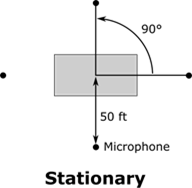

For stationary noise sources, measure a 30-second LAeq at each of the four azimuth angles. Use shorter durations if the sound level is relatively steady as a function of time and if a 30-second measurement is not possible. For mobile noise sources, measure the maximum A-weighted sound pressure level with fast exponential time averaging (LAFmx). The individual reference levels and the number and type of each piece of construction equipment are then, ultimately, used to compute the total equivalent sound level, LAeq,total, for a typical work day during a particular construction phase. Other descriptors can be computed using the mathematical relationships presented in Appendix A. The LAeq descriptor may be more useful in assessing potential noise impact due to construction-related activity.
Vibration from construction equipment is characterized for two different purposes: human response and building response. Use construction noise descriptors—but with a flat weighting—to characterize human response. Measure the 30-second Leq for stationary sources. Consider longer measurement periods if low-frequency vibration (below 5 Hz) is a concern. Measure the maximum vibration velocity level LFmx for mobile sources.
High levels of groundborne vibration caused by construction equipment may cause building damage and necessitate assessment. Levels for building damage are compared to PPV. PPV can be measured using the same transducers at the same positions as noise and vibration Leq. Both Leq and PPV can be calculated from the recorded waveform data. If the recording device does not record the signal directly (e.g., sound level meter), then the device should be set to log both Leq and PPV simultaneously.
The FHWA Roadway Construction Noise Model (RCNM) currently uses broadband noise levels; however, a future version is expected to include one-third octave band noise data. It is possible that the model could be extended to include one-third octave band vibration data and predictions. For these reasons, measuring construction noise and vibration one-third octave band emission levels could help with modeling. Evaluate applicable metrics for the RCNM input capabilities to determine additional measurement metrics requirements.
The instrumentation for measuring construction equipment noise and vibration is the same as for measuring existing or traffic noise and vibration. See Section 3.3, Section 4.3, and Section 7.3 for additional information.
Some sound level meters can use geophones or accelerometers as inputs. These meters will usually have options to convert acceleration inputs to velocity and to directly record unweighted level descriptors and PPV. If these options are unavailable, then a different device should be used to record the measurement. Similarly, for seismographs, the device must record the appropriate level descriptors or the recorded waveform must undergo postprocessing.
A multichannel recording system should be used when measuring noise and vibration for the same equipment in the same operating mode. This will aid in identifying and correlating noise and vibration data from different events.
Meteorological data are generally not needed for vibration measurements. However, avoid vibration measurements if it is raining, if soil is atypically saturated with water, or if the ground is frozen.
The sampling period varies for each type of construction equipment depending on the operating mode (“stationary-passive,” “stationary-active,” “mobile-passive,” and “mobile-active”). During the measurement, appropriate personnel should operate the equipment in a manner that is considered typical for the work period and operating mode. Due to construction site activity, the sampling period may be based entirely on good engineering judgment; the person performing the measurements is responsible for obtaining representative, high-quality data.
The steps below describe what needs to be done upon arrival at the site, on through the successful collection of data.
Exact data analysis and reporting requirements will vary by project sponsor. However, typical data analysis and reporting procedures are shown below for the noise data analysis and, as applicable, the vibration data analysis.
where Li is the ith good second’s Leq and n is the total number of good seconds.
CAL adjustment = Reference level - [(CALINITIAL + CALFINAL) / 2]
For example, if:
Reference level (manufacturer’s calibration level) = 114.0 dB
Initial calibration level = 114.0 dB
Final calibration level = 114.4 dB
Then:
CAL adjustment = 114.0 - [(114.0 + 114.4)/2] = -0.2 dB
In this example, adjust the measured Leq downward by 0.2 dB, with a note that it has been adjusted.
If the total measured level exceeds the background level by between 5 and 10 dB, then the measured level should be adjusted for background noise to get the source-only level as follows:
Equation 8-2: Formula for Adjusting Leq for Background
where: Ladj is the background-adjusted measured level;
Lc is the total measured level with source and background combined; and
Lb is the background level alone.
For example, if:
Lc = 55.0 dB
Lb = 47.0 dB
Then:
Equation 8-3: Example of Background Adjustment
 = 54.3 dB
The total equivalent sound level for a typical work day during a particular construction phase is computed as follows:
Equation 8-4: Formula for LAeq Over Time
![LAeq, total equals 10 times the log base 10 of sum from i equals 1 to K [10 raised to the power of LAeq, i divided by 10].](image015.png)
where: LAeq,total is the total equivalent sound level for a typical work day during a particular construction period;
k is the number of different types of equipment; and
LAeq,i is the equivalent sound level for equipment type i.
For example, given:
LAeq,1 = 89.0 dB
LAeq,2 = 81.7 dB
LAeq,3 = 79.0 dB
LAeq,4 = 80.5 dB
Therefore:
Equation 8-5: Example of Leq Addition

This section describes recommended procedures for the measurement of highway noise barrier insertion loss (IL). IL is the difference in sound level at a receptor location with and without the presence of a noise barrier, assuming no change in the sound level of the source.
The following project types could use highway noise barrier IL measurement procedures:
The procedures described in this section are in accordance with ANSI/ASA S12.8-1998 (R2013),[58] which provides three methods to determine the field insertion loss of noise barriers:
Direct Measured: The direct measured BEFORE/AFTER method requires making site measurements before the barrier has been constructed to determine BEFORE levels; it also requires another set of measurements at the same site after construction to determine AFTER levels. This method ensures identical site geometric characteristics if there have not been any changes to the roadway’s cross-sectional geometry, such as a widening of the roadway. However, this method also requires equivalent BEFORE and AFTER meteorological and traffic conditions that may be difficult to reproduce.
Indirect Measured: The indirect measured method requires performing measurements at a site with a barrier to determine AFTER levels; it also requires another set of measurements at an “equivalent” site without a barrier to determine equivalent BEFORE levels.
Judge a site as equivalent if geometric, meteorological, and traffic conditions are essentially identical for the BEFORE case as compared with the AFTER case. Geometric equivalence refers to the terrain characteristics and ground impedance at the site, including pavement type and condition. Meteorological equivalence refers to temperature lapse rate (the change in temperature with increasing height above ground), wind speed and direction, and—to a lesser degree—temperature and humidity (see Section 9.1.1.2). Traffic equivalence refers to vehicle volumes (by type of vehicle) and speed.
For the indirect measured method, the BEFORE and AFTER measurements are best made simultaneously at adjacent sites to ensure essentially the same meteorological and traffic conditions for both sets of measurements. However, finding an adjacent equivalent site may be difficult. If the selected site is not adjacent or the measurements ae not simultaneous, then: 1) adjustments will likely be needed for equivalence of traffic, with the possible introduction of some error if vehicle mix or speed is different; and 2) meteorological conditions may not be equivalent, including wind direction if the roadways at each site are not oriented the same relative to north.
Indirect Predicted: The indirect predicted method uses measurements at a site with a barrier to determine AFTER levels. It also uses a highway traffic noise prediction model such as FHWA TNM to predict BEFORE sound levels at the same site without the barrier. The first disadvantage of this method is that it presumes the accuracy of a model for this particular site instead of using actual measurements for the BEFORE condition. The second disadvantage of this method, at least in the case of FHWA TNM, is that it can only be used when AFTER levels have been measured under neutral meteorological conditions (no wind and no change in temperature with height above ground), since FHWA TNM only models for neutral conditions.
Site selection for all three measurement methods is guided by site geometry and the location of receptors of interest. Site selection is also driven by the goals of the study—in this case, to determine the IL of a noise barrier at receptors of interest. There are two aspects to consider regarding site selection:
The location of a planned or existing noise barrier of interest and, for the indirect measured method, an equivalent No-Barrier BEFORE site determine site selection. Establish equivalence in site geometry, meteorological conditions, and traffic conditions for valid comparison of BEFORE and AFTER sound levels. Use highway plans, land-use maps, aerial photos, including web-based mapping sites, and field reconnaissance to identify candidate sites.
Equivalence in site geometry entails similar terrain characteristics and ground type within an angular sector of at least 120° and preferably 140° from all measurement points looking toward the noise source. Important terrain characteristics include the following:
Identify the presence of paved areas or water, which affect measured levels. For research purposes, equivalence in ground impedance may be determined by performing measurements in accordance with the ANSI/ASA S1.18-2010,[59] which, among other methods, is discussed in Section 9.1.2.1.
For more empirical studies, or if ground impedance measurements are not feasible, then judge the ground for BEFORE and AFTER measurements as equivalent if general ground surface type and conditions (e.g., surface water content) are similar. Ground surface guidance is found in Ground and Pavement Effects using FHWA’s Traffic Noise Model 2.5,[60] which is repeated in NCHRP Report 791.[61]
Additionally, the presence of noise sources other than the roadway of interest, including other roads, rail lines, airports, industrial or commercial operations, and temporary construction, repair, and maintenance activities could make the direct or indirect BEFORE site not equivalent to the AFTER site. An exception would be if the measurements can be done when these sources are not operating.
Equivalence in meteorological conditions includes the following:
Wind: Wind affects measured sound levels in two ways:
Judge wind conditions equivalent for BEFORE and AFTER measurements if
VWS is computed as:
VWS = (Wind Speed) x cos(Wind Direction)
It is possible to calculate a VWS under 2.2 mph (1.0 m/s) when strong winds are nearly parallel to the roadway. However, this condition is not truly a “calm” case. In other words, avoid BEFORE/AFTER measurements in such instances.[63] A negative VWS indicates the wind is blowing from the sound level measurement point to the source (the upwind class).
| Wind Class | Vector Wind Speed (mph) |
|---|---|
| Upwind | -11 to -2.2 |
| Calm | -2.2 to +2.2 |
| Downwind | +2.2 to +11 |
Table 9-1 note: 1 mph = 0.45 m/s.
Temperature lapse rate: The changing of temperature with height above the ground (“temperature lapse rate”) can have a major effect on measured sound levels and IL by refraction, especially at greater distances from the source.[64] For the same traffic volume, speed and vehicle mix, levels would be higher on clear nights during inversions (temperature increasing with height above ground). The levels would be lower during bright, sunny days (temperature decreasing sharply with height above ground) compared to a neutral atmosphere (no change in temperature with height). Neutral conditions are usually only seen briefly around sunrise and sunset).
For research studies, measure temperature lapse rate during the sound level measurements. Measurement of temperature at two heights above ground—such as 5 ft and 15 ft (1.5 m and 4.6 m)—is a precise way to determine lapse rate and the likelihood of refraction. Section 4.4.1 presented characterizations or classes of the lapse rate per guidance in NCHRP Report 791:[65] 1) strong lapse; 2) weak lapse; 3) neutral; 4) weak inversion; and 5) strong inversion. For this measurement procedure, it is sufficient to characterize lapse rate by one of three conditions:
For more empirical studies, as an alternative to measuring and using the lapse rate to help determine equivalence, make the BEFORE and AFTER acoustical measurements under the same class of cloud cover. Table 9-2 describes these classes.
Temperature and humidity: Judge average temperatures during BEFORE and AFTER measurements equivalent if they are within 25° F (14° C) of each other. Also, in certain conditions, dry air produces substantial changes in sound attenuation at high frequencies. Therefore, for a predominantly high-frequency source (most sound energy over 3,000 Hz, which would not be traffic noise), ensure that the absolute humidity for BEFORE and AFTER measurements are similar.
Equivalence in traffic conditions includes the following:
To a certain degree, nonequivalence in traffic conditions can be factored out through the use of a reference microphone (Section 9.1.2.1). There may be some differences for BEFORE and AFTER measurements in spectral content, directivity, and spatial and temporal patterns of the individual vehicles, but this is usually not an issue in most traffic situations. However, discard data that include unrepresentative or unusual vehicle sounds.
If possible, use a reference microphone for all barrier insertion loss measurements at both the Barrier and No-Barrier sites. Using reference microphones allows for a calibration of measured levels, which helps to account for variations in the characteristics of the noise source (e.g., traffic speeds, volumes, and mixes).
Place the reference microphone in the same position as in the AFTER case for the BEFORE measurements for the direct measured method and for the equivalent BEFORE measurements for the indirect measured method. If the barrier is located 50 ft (15.2 m) or more from the center of the near travel lane, then place the AFTER reference microphone at a height of 5 ft (1.5 m) directly above the top of the barrier. (Figure 9-1).
If the barrier is located less than 50 ft (15.2 m) from the center of the near travel lane, then place the reference microphone at 50 ft (15.2 m) from the center of the near travel lane, at a height such that the line of sight angle between the microphone and barrier top, as measured from the center of the near travel lane is at least 10° (Figure 9-2). It may not be practical to use this latter position because of the microphone height that might be required, especially for tall noise barriers at the roadway shoulder. In such a case, the measurement may be performed without the reference microphone at the Barrier site if the equivalent No-Barrier (BEFORE) site is adjacent to the Barrier site, because the traffic will be the same at the two sites.
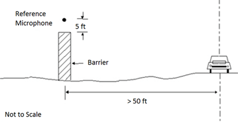
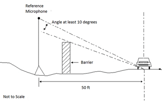
When determining barrier insertion loss, the receiver microphone locations should be identical in the BEFORE and AFTER cases in terms of distance from the road and height above the road. In most situations, study objectives will dictate microphone locations. As such, this section presents a generic discussion of microphone locations, and assumes no specific study objectives have been identified. However, the same locations where existing noise measurements might be made as part of a traffic noise study could be places of interest for measuring barrier insertion loss.
The preferred microphone height is 5 ft (1.5 m) above the ground. It may be helpful to include microphones at representative heights of balconies [plus 5 ft (1.5 m)] or at window height if multistory structures are of interest. Lacking specific points of interest, it may be helpful to position receiver microphones at offset distances from the barrier that correspond to incremental doublings of distances [e.g., 50 ft, 100 ft, and 200 ft (15 m, 30 m, and 60 m)] and at multiple heights at each offset distance. For receiver distances greater than 300 ft (100 m) from the source, atmospheric effects have a much greater influence on measured sound levels than at closer distances.[66] Obtain precise meteorological data in such instances to ensure BEFORE and AFTER equivalence of the meteorological conditions.
Use the equivalent sound level (Leq) for determining the noise barrier insertion loss for traffic. Use the SEL (LAE), or the maximum A-weighted sound level with fast time response characteristics (LAFmx), if the goal is to describe the sound of single events, such as individual vehicle pass-bys.
The DNL (Ldn) and the CNEL (Lden) may be used to describe long-term noise environments (typically greater than 24 hours), particularly for land-use planning. However, given the requirements of source and meteorological equivalence for the BEFORE and AFTER measurements, it would extremely difficult to measure a barrier’s IL for DNL or CNEL. An exception could be for the indirect measured method if the BEFORE and AFTER sites were adjacent to each other, with the roadway oriented in the same direction relative to north at each site. Even then the IL would almost certainly be for a mixed set of meteorological conditions. DNL and CNEL can be computed using the mathematical relationships presented in Appendix A once the Leq and LAE noise descriptors are established.
Appendix B provides information and a discussion on instrumentation, as well as other useful accessories and field supplies.
Consider three factors when selecting a sampling period:
The goal of these measurements is to determine the IL of traffic noise provided by an in-place noise barrier of choice and possibly under meteorological conditions of choice. These measurements do not need to be made during the worst noise hour. Avoid measurement when traffic flow is congested because the traffic noise level will be lowered, making it more difficult to determine the full amount of the IL.
A key aspect of the “when to measure” question relates to meteorological conditions of interest, which can substantially affect both measured sound levels and noise barrier IL, as discussed in Section 9.1.1.2. Conduct BEFORE and AFTER measurements under equivalent meteorological conditions for comparability. Essentially, with the key factors being wind shear and temperature lapse rate, nine meteorological “classes” can be described: upwind (with negative, neutral, or positive lapse rate); calm (with negative, neutral, or positive lapse rate); and downwind (with negative, neutral, or positive lapse rate). Using lapse rate categories of strong and weak results in further classification division.
The meteorological class can change several times over one day, especially with changes in wind direction. The class that will occur during measurements cannot reliably be determined in advance.
In addition to the effects of wind direction on equivalence, wind can flutter the microphone diaphragm and produce false noise readings (even through a proper windscreen). Do not make sound level measurements when winds exceed 11 mph (17 kmh or 5 m/s), regardless of direction (or delete any data collected during such periods during data analysis). If the A-weighted sound levels are lower than 40 dBA, even lower-speed winds can cause false noises.
Finally, avoid sound level measurements during precipitation or when the pavement is wet. Aside from being bad for equipment, rain drops can generate noise on leaves, metal roofs, and plastic bags that have been placed over microphone windscreens and instruments. Tire noise increases on wet pavements, especially in the higher frequencies that most affect an A-weighted sound level.
Unlike some of the other measurement procedures, the goal is not to represent the one-hour LAeq with a shorter-term measurement, but rather to determine a level difference, the IL. A key consideration in choosing a measurement duration is the proper representation of the spectrum of the traffic noise, so that the A-weighted IL is accurately determined.
Because it is largely impossible to determine the meteorological class(es) in advance, one technique is to measure sound levels, wind speed and direction and temperature lapse rate for a four-hour block of time in one-minute increments.[68] This block of time could be extended beyond four hours depending on the study requirements and time and budget permitting. Then, the data are broken down into five-minute periods and the Leq and meteorological class are determined for each five-minute period.
Additionally, traffic data varies over time. Assign each of the five-minute time periods to a traffic class based on similarities in traffic volume, mix, and speed. Assign some of the five-minute periods into groups of equivalent periods by jointly examining traffic and meteorological classes.
If traffic is intermittent, then the difference in traffic parameters from one five-minute period to the next may be too large to characterize any of the periods as equivalent. In such a case, extend the period duration to 10-minutes or longer, which is possible if the data have been collected in one-minute intervals.
Repeating a measurement more than once will help address result variability concerns. As noted, this procedure determines the noise barrier IL, not a representative one-hour Leq; thus, there should be less variation in the result. Collect and average at least three periods of equivalent data—in terms of traffic and meteorological class—to determine the IL for a set of conditions. If measuring four or more hours of data (as discussed previously), then it may be possible to describe the IL of the noise barrier for multiple sets of equivalent traffic and meteorological conditions.
This section presents the measurement procedure. More specific details for the persons going into the field are in the FHWA Noise Measurement Field Guide. Prior to traveling to conduct the sound level measurements, plan the measurement study as described in Section 2.0, preferably with a thorough field review. Careful advanced planning of microphone locations, heights, and the needed microphone support mechanisms (tripods, tall tripods or masts with guy-wire systems) is crucial, as are suitable and safe locations for counting of traffic and sampling of speeds. The following steps apply for all methods except the BEFORE predictions for the indirect predicted method, which is discussed separately in Section 9.6.
The steps below describe what needs to be done upon arrival at the site, on through the successful collection of data.
Intermittent traffic flow: It may be possible to measure the background sound level in the absence of traffic. Sampling duration depends on the temporal nature of the background noise:
Continuous traffic flow: The background level cannot be determined. Judge whether any background noise sources cause an increase in the total measured level. Audibility of background noise source is one important factor. If inaudible, then it is likely that background noise is not affecting the total level. If background noise is audible, then do not use the one-minute intervals in which it is audible in the data analysis.
Appendix B provides details on different types of equipment and techniques for measuring speed.
Documentation is an essential part of every measurement. There are two stages to documentation: 1) in the field; and 2) after data analysis. This section describes field documentation. Field data sheets and more specific guidance are in the FHWA Noise Measurement Field Guide. Complete data sheets in the field while at the site. Make documentation sufficient for another person to return to that same microphone location and repeat the measurement with the same equipment and settings and under the same conditions. Here are some parameters to document using data sheets:
Modeled levels at the reference position may differ substantially in the predicted BEFORE case from the measured AFTER case. In such instances, consider using the Continuous-Flow Traffic Time-Integrated Method (CTIM) procedure described in Section 13.0 to normalize for different traffic conditions.
Establish the equivalence of meteorological conditions (i.e., wind, temperature, humidity, and cloud cover) for valid comparisons of BEFORE and AFTER measured levels (see Section 9.1.1.2). This section assumes that equivalence of site parameters, such as terrain characteristics and ground impedance, was established prior to performing measurements. Exclude from subsequent analysis sampling periods without established equivalence.
where Li is the ith good minute’s Leq and n is the total number of good minutes.
CAL adjustment = Reference level - [(CALINITIAL + CALFINAL) / 2]
For example, if:
Reference level (manufacturer’s calibration level) = 114.0 dB
Initial calibration level = 114.0 dB
Final calibration level = 114.4 dB
Then:
CAL adjustment = 114.0 - [(114.0 + 114.4)/2] = -0.2 dB
In this example, adjust the measured Leq by 0.2 dB, with a note that it has been adjusted.
As an alternative, if collecting a long block of data (e.g., the four hours described in this section) and dividing those data into discrete short-term periods, consider adjusting the data assuming a linear drift in the calibration over the duration of the data collection. To do this, calculate time-based adjustments and apply them to each short-term period. In the example above, the assumption would be to adjust data collected in the first hour less than data collected in the last hour, instead of all data being adjusted by -0.2 dB.
For these reasons, consider applying a -0.5 dB bias adjustment to the Position 1 reference microphone sound levels in the AFTER case.[69] Use good engineering judgment—based on repeatability through measurements—to determine the magnitude and necessity of this adjustment. This is particularly relevant to the indirect measured method where the equivalent BEFORE site is adjacent to the AFTER site and the traffic passing both sites is the same at both sites. For example, if for several measurement periods, a consistent repeatable difference at the reference microphone position in the equivalent BEFORE and AFTER case occurs, and it can be shown that the traffic during both cases were equivalent, then the difference can be attributed to reflection or edge-diffraction effects.
Larger corrections may be necessary for situations with parallel barriers on both sides of the road, if evidenced in repeated measurements of the equivalent BEFORE and AFTER cases where traffic is equivalent. Alternatively, consider using FHWA TNM’s Parallel Barriers module to determine a multiple-reflections increase due to the parallel barriers that would be in addition to the -0.5 dB source reflections/edge-diffraction bias.
ILi = (LAref + Ledge - LArec) - (LBref - LBrec) (dB)
where:
ILi is the IL at the ith receiver;
LBref and LAref are, respectively, the BEFORE and AFTER adjusted reference levels;
Ledge is the reflections/edge-diffraction bias adjustment, if used; and
LBrec and LArec are, respectively, the BEFORE and AFTER adjusted source levels at the ith receiver.
For example, if:
LAref = 78.2 dB
Ledge = -0.5 dB
LArec at Receiver 1= 56.3 dB
LBref = 77.7 dB
LBrec at Receiver 1= 65.0 dB
Then:
IL1 = (78.2 - 0.5 - 56.2) - (77.7 - 65.0) = 21.5 - 12.7 = 8.8 dB
This section describes recommended procedures for the measurement of vehicle noise emission levels. Do not use these procedures for determining existing sound levels or validating FHWA TNM as part of a traffic noise study done under 23 CFR 772. Instead, use these specialized procedures to accomplish the following:
The procedures described in this section are consistent with the methodology used during the development of the Reference Energy Mean Emission Levels (REMEL) database for FHWA TNM.[71] Section 10.6.1 discusses the methodology for developing the REMEL equations.
FHWA TNM groups vehicles into five acoustically significant types (i.e., vehicles within each type exhibit statistically similar acoustical characteristics). These vehicle types, defined in Section 4.5.1, are automobiles, medium trucks, heavy trucks, buses, and motorcycles. The FHWA TNM User Guide states the following policy: “TNM allows the user to input data and calculate noise levels utilizing user-defined vehicle types. This feature should only be used for unique vehicle types which differ substantially from the five standard vehicle types contained in TNM, e.g., recreational vehicles or electric vehicles. It should not be used to input State-specific emission levels for the five standard vehicle types.”
After determining the REMEL equation parameters for input into TNM, the noise analyst must choose one of the five standard vehicle types as being most similar to the user-defined vehicle type. FHWA TNM then assigns the spectral and source height characteristics of that standard type to the user-defined vehicle type. Be aware that, in reality, the spectral and source height characteristics of the new vehicle type may differ from those of the five standard types. For example, is the spectrum for an electric vehicle similar to those of the gasoline- or diesel-powered vehicles that comprise TNM’s automobile vehicle type, especially at low speeds?
Before conducting a study to develop REMEL equations, review Appendix B of FHWA Traffic Noise Model (TNM) Pavement Effects Implementation Study: Progress Report 1[72] and consult with FHWA. The report’s Appendix B addresses a number of important problems regarding the sufficiency and validity of the collected database and resulting emission level equations:
Site selection is driven by the goals of the study—in this case, to measure vehicle noise emission levels. There are two aspects to consider regarding site selection:
Use highway plans, land-use maps, aerial photos, including web-based mapping sites, and field reconnaissance to identify candidate sites. Select 5 to 10 unique sites to minimize site-specific effects associated with vehicle noise emission level measurements. Also choose a site for measuring idling vehicles.
These sites should possess the following characteristics:
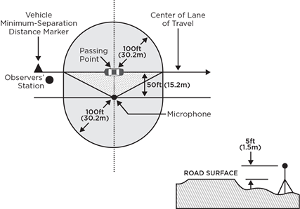
Place the microphone 50 ft (15.2 m) from the center of the near travel lane, with the microphone diaphragm positioned for grazing incidence at a height of 5 ft (1.5 m) above the plane of the roadway surface (Figure 10-1). If the ground slopes up from the roadway to this location, then maintain a minimum height of 5 ft (1.5 m) above the ground, even if it results in the height of the microphone being greater than 5 ft (1.5 m) above the plane of the roadway surface. Note the microphone height above the roadway plane. Position additional microphone systems at other offset distances [e.g., 100 ft and 200 ft (30 m and 60 m)] if characterizing the sound level drop-off rate at the site is a goal of the measurement study.
The maximum A-weighted sound pressure level with fast exponential time averaging (LAFmx) is used for the development of vehicle noise emission level relationships. Additionally, one-third octave band spectral data from 25 Hz to 10,000 Hz will be useful during analysis. While spectral data are not required for creating a user-defined vehicle type in FHWA TNM, the program’s computations are performed in one-third octave bands. Since the FHWA TNM user must assign the spectral characteristics of one of the five standard vehicle types to the user-defined type, it is important to verify consistency with the spectral data currently in the model.[73] Spectral data are also essential if data are being collected as part of a research project to characterize REMELs on different pavement types.
Measuring vehicle noise emission levels is different from measuring the Leq of a stream of traffic. Measuring vehicle noise emission levels requires “clean” pass-bys of individual vehicles, unaffected by noise from other vehicles traveling in the same direction or in the opposite direction. Specifically, the ideal difference between the lowest anticipated LAFmx for a vehicle pass-by and the A-weighted background level, as measured at the 50-ft (15.2-m) microphone, is at least 10 dB. The sampling period for each vehicle pass-by varies, but the period should encompass a minimum rise and fall in the sound level time-history trace of 6 dB, with 10 dB being preferred (Section 10.4.1 and Appendix D). Rise and fall are defined, respectively, as the difference between LAFmx and the minimum measured level associated with either the start or end of a given pass-by (whichever difference is smaller). This criterion ensures the quality of the pass-by event, and may be determined by: 1) observing the display of the sound level meter; or 2) examining the time history (instantaneous LAFmx as a function of time) if the sound level instrument has the capability of displaying and storing that time history.
The event quality for each pass-by can be affected by the presence of background noise or nearby vehicles, which can affect the measured maximum level during the subject vehicle pass-by and the rise and fall of the level during the pass-by. Determine event quality during data measurement and prior to data analysis using three type designations (Type 2, 1, or 0):
In special situations where it is difficult to find ideal sites, the analysis can include lower-quality events, such as events in which the background is less than 10 dB below the LAFmx.
Type 1 events in which the background is less than 10 dB below the LAFmx: There may be situations where it is necessary to relax the 10-dB background requirement to 6-dB. Examples are during the measurement of low-speed automobiles or during the measurement of infrequent vehicle types, such as buses. Correct the LAFmx for these events for background via energy-subtraction before data analysis as follows:
Equation 10-1: Formula for Adjusting Leq for Background
where:
Ladj is the background-adjusted measured level;
Lc is the measured level with vehicle and background combined; and
Lb is the background level alone.
For example, if:
Lc = 55.0 dB
Lb = 47.0 dB
Then:
Equation 10-2: Example of Background Adjustment
= 54.3 dB
Use a minimum separation distance between vehicles during event selection in the field. This will ensure negligible contamination from vehicles other than the subject vehicle (either leading or following the subject vehicle traveling in the same direction or traveling in the opposite direction). Appendix D presents a procedure for determining and using this minimum separation distance. Minimum separations differ by vehicle type. If trying to measure an automobile with a leading or following heavy truck, the separation should be at least twice as much than as if the other vehicle was a car (assuming heavy trucks are approximately 10 dB louder than automobiles). If trying to measure a heavy truck with a leading or following automobile, then the separation should be much less than if the other vehicle was a heavy truck. If microphones are also to be positioned farther from the road, then the separation distances should be greater to avoid contamination from nearby vehicles.
Table 10-1 provides, as a function of speed, the recommended minimum number of samples.[75] While the number of samples is somewhat arbitrary and often a function of budgetary constraints, a larger number of samples will result in higher precision and a greater degree of statistical confidence in the final emission levels. Report 1 for discussion on sample sizes and distribution over the speed range of interest.[76]
Note that collecting the minimum number for frequent vehicles like automobiles and heavy trucks may be easy, it could difficult and impractical for less frequent vehicles like medium trucks, buses, and motorcycles. As a point of relative comparison, 2,825 automobiles, 765 medium trucks, 2,986 heavy trucks, 355 buses, and 39 motorcycles were sampled on a total of three different general pavement types in the development of FHWA TNM. Do not exclude samples that appear to be outliers (e.g., extremely loud vehicles) in the dataset; the data collected should be representative of a random sample because the field measurement procedure uses the minimum separation-distance criteria.
This section presents the measurement procedure. More specific details for the person going into the field are in the FHWA Noise Measurement Field Guide. Prior to traveling to conduct the sound level measurements, plan the measurement study, as described in Section 2.0. In the case of vehicle emission-level measurements, the project sponsor SHA should coordinate with FHWA during the study conception and planning should be done.
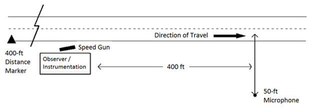
Documentation is an essential part of every measurement. There are two stages to documentation: 1) in the field; and 2) after data analysis. This section describes field documentation. Data sheets and more specific guidance for the person going into the field are in the FHWA Noise Measurement Field Guide. Complete data sheets in the field while at the site. Make documentation sufficient for another person to return to that same microphone location and repeat the measurement with the same equipment and settings and under the same conditions. Here are some parameters to document using data sheets:
CAL adjustment = Reference level - [(CALINITIAL + CALFINAL) / 2]
For example, if:
Reference level (manufacturer’s calibration level) = 114.0 dB
Initial calibration level = 114.0 dB
Final calibration level = 114.4 dB
Then:
CAL adjustment = 114.0 - [(114.0 + 114.4)/2] = -0.2 dB
In this example, adjust the measured Leq downward by 0.2 dB, with a note that it has been adjusted.
As an alternative if a long block of data has been collected (e.g., over several hours) and those data are being divided into discrete short-term periods, consider adjusting the data assuming a linear drift in the calibration over the duration of the data collection. To do this, calculate time-based adjustments and apply them to each short-term period. In the example above, the assumption would be to adjust data collected in the first hour less than data collected in the last hour, instead of all data being adjusted by -0.2 dB.
FHWA TNM allows the program’s user to input user-defined vehicles. FHWA’s current policy is that this capability is not for entering state-specific emission levels, but for representing new vehicle types other than the standard five in FHWA TNM. Before proceeding with the data analysis, consult with FHWA for the latest procedures, because what is presented below is subject to change.
Developing the overall A-weighted REMEL equation for a user-defined vehicle type involves two basic steps:
Then, determine the four needed input parameters for specifying the user-defined vehicle in FHWA TNM.
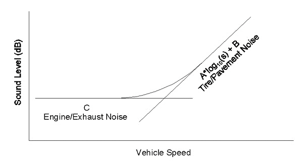
L(s) is the level of the combined levels of a constant, C, representing the engine/exhaust component, and [A log10(s) + B], representing the tire/pavement component. The functional form of the “level-mean” regression equation is represented as follows:
Equation 10-3: Functional Form of the “Level-Mean” Regression Equation

 , separately for each component (idle/low speeds and higher speeds):
Equation 10-4: Formula for Linear Average of All Samples

where:
Li represents the level of the ith sample, and
N represents the total number of data samples.
Equation 10-5: Formula for Residuals between Samples and Level-Mean

where: ri equals (ri)c or (ri)b, depending on the component source data (respectively, idle/low-speed and higher-speed).
Equation 10-6: Formula for Level-Mean to Energy-Mean Adjustment Factor
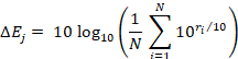
Equation 10-7: Formula for Energy-Mean Emission Level Regression Equation

For example, assume
C = 50.128
A = 41.741
B = 1.149
ΔEc= 2.26725
ΔEb = 0.925
s = 65 mph (105 kmh) (if metric units are used, then s is divided by 1.609 in the equation to convert to an English value).
Then:
Equation 10-8: Example of Energy-Mean Calculation

From the above energy-mean emission-level regression equation, four input parameters are required to specify a user-defined vehicle type in the FHWA TNM:
A similar vehicle type is one of the five FHWA TNM vehicle types to which the user-defined type is most alike. In determining the similar vehicle type, the factors to be considered, in order of importance, are: estimated sub-source heights; estimated acceleration characteristics; and estimated one-third octave band frequency spectrum.[77]
There are two standardized methods of directly measuring tire-pavement noise source levels: the close-proximity (CPX) method and the on-board sound intensity (OBSI) method. These procedures isolate tire noise generation from other sources of the exterior vehicle noise. These other sources include items such as powertrain noise due to the engine, exhaust, transmission, and other driveline components, and noise generated aerodynamically due to air flow around and underneath the vehicle body.
The tire-pavement noise measurement methods use a vehicle or vehicle with trailer to collect data on in-service highway lanes or test roadways, which allows for acquisition of data at any desired location along a roadway, or any travel lane, assuming all method criteria are met. These methods have limitations, including limited tire type representation and inability to account for porous pavement effects on sound propagation (as experienced by receptors adjacent to roads).
Here are the types of projects to which the methods apply:
The ISO CPX method [International Organization of Standardization (ISO) 11819-1, Acoustics—Measurement of influence of road surfaces on traffic noise—Part 2: The close-proximity (CPX) method] was the first at-the-source procedure to be standardized on a national/international level. This procedure requires the use of a special test vehicle or test trailer designed to meet specific acoustic performance standards. Two required microphone locations are specified 7.9 in (200 mm) outboard of the plane of the tire sidewall. The sound pressure levels measured by these microphones at specified speeds are averaged together to define a reported CPX level. Standard test tires are used for the measurements.
The ISO CPX was developed in the late 1990s to quantify the level of tire-pavement noise produced in situ by an in-service pavement. The draft procedure was published in 2000 and was released as a standard in 2017. Changes include the specifications of the trailer/vehicle used, the standard test tires, corrections for temperature, correction for test tire hardness, and the reduction of potential uncertainties. Currently, there are three alternatives for measurement apparatus: an enclosed test trailer, an open test trailer, and a self-powered vehicle. An enclosed trailer is intended to reduce the effects of wind on the measurement microphones and noise contamination of other vehicles on the roadway under test. Requirements are placed on the enclosed trailer design to minimize the effect of the reflections inside the enclosure, background noise from the towing vehicle, and the second non-test tire for a two-wheel trailer. Open trailers are required to meet the same specifications with additional consideration for wind noise on the microphones. For self-powered vehicles, there are additional requirements on where the test tire is mounted and additional recommendations regarding vehicle treatments.
The ISO CPX method has had extensive development in Europe for almost 20 years. Much of the quieter pavement research done in Europe and Asia has used the CPX method, resulting in a wealth of method data. Several studies have been reported in the literature regarding the relationships between CPX data and the ISO SPB method [ISO 11819-1, Acoustics—Measurement of influence of road surfaces on traffic noise—Part 1: Statistical pass-by (SPB) method; see Section 12.0 for more information on the SPB method]. Because the CPX method measures sound pressure level, the results of CPX measurements on porous pavement include some of the effects of pavement sound absorption, which can help in pass-by correlation for these pavements. The CPX method also uses different tires to represent light and heavy vehicle tire-pavement noise. The actual noise measurements for the CPX method are quite simple, relying only on a measurement of sound pressure level.
One of the significant drawbacks of the CPX procedure is the use of a trailer or special self-powered vehicle. For the two different types of trailer, open and enclosed, there is the expense of building, qualifying, maintaining, and storing the trailer. With a trailer, different tow vehicles could be used so that a dedicated vehicle is not needed if a new tow vehicle does not introduce interfering background noise. A self-powered vehicle also must be qualified and possibly treated with acoustical material, which can require dedicating a vehicle to the CPX measurement. Further, it may be difficult to find a self-powered vehicle that will accommodate all the test tire sizes and provide the required tire loading.
The American Association of State Highway Transportation Officials (AASHTO) Standard Method of Test Measurement of Tire/Pavement Noise Using the OBSI method evolved from a procedure adapted for use in Caltrans in their Quieter Pavement Research projects in the early 2000s. These projects evaluated pavements for noise performance. The application of sound intensity to tire noise measurement was originally developed at General Motors for tire noise research and specification in the early 1980s. The procedure applies microphones suspended from a fixture mounted to the tire/wheel hub directly on a test vehicle. Two closely spaced microphones forming an intensity probe measure sound intensity at two locations 3.9 in (100 mm) outboard of the leading and trailing edges of the tire contact patch. The sound intensity readings measured by these probes are averaged together to determine the reported OBSI level at a standardized speed of 60 mph (96.6 kmh). A standard test tire is used for measurement.
The OBSI procedure was adapted by AASHTO as a full standard in 2016 and designated T360-6 after being referred to as TP76 while it was a provisional standard. T360-6 was developed by a FHWA Working Group beginning in the mid-2000s. The FHWA Tire-Pavement Noise Strategic Planning Workshop, held in September 2004, identified the need for a common on-board, at-the-tire-pavement source measurement procedure. Two NCHRP projects, which were completed in the mid to late 2000s, supported this need. The first project evaluated at-the-source methods and recommended the OBSI approach.[78] The second project evaluated measurement variables and established precision and bias statements.[79]
Under the OBSI procedure, the method for suspending the intensity probes in position is not defined; however, practitioners typically use a fixture attached to the wheel hub using lug nut extensions in place of some of the normal lug nuts. The procedure does not require a specific or dedicated test vehicle; however, it must accommodate the test tire and wheel, be mounted on a non-driven, non-steering axle, and provide the required tire loading range as it is or with added weight. If the vehicle meets the requirements, then it is not necessary to use the same vehicle for repeated measurements.
In addition to the probes being 3.9 in. (100 mm) from the deflected tire sidewall, they are 3 in. (77.2 mm) above the pavement. The two probes are 8.25 in. (209.6 mm) apart horizontally, which positions the probes directly opposite the leading and trailing edges of the tire contact patch. The preferred standard test speed is 60 mph (96.6 kmh) with acceptable alternatives of 45 mph, 35 mph, and 25 mph (72.4 kmh, 56.3 kmh, and 40.3 kmh). One test tire is specified: the ASTM Standard Reference Test Tire (SRTT) F2493, which is the same as that adopted by the CPX procedure. Studies have found that the ASTM SRTT represents heavier highway vehicles without requiring additional tire designs. The standard defines required tire inflation pressure, tire rubber hardness, and tire loading. The standard also provides data quality indicators that must be met, including the direction of the intensity vector coming from the tire, the ratio of sound pressure level to sound intensity level (PI index), the coherence of the pressure signals for the two microphones comprising a sound intensity probe, and the allowable variation from run-to-run. A standard test section length is 440 ft (134.1 m), and an energy average is to be made over this length. The levels from the leading and trailing edge probes employ energy basis averages and require at least two measurements of the same section. The standard also includes a temperature correction method.
Since the mid-2000s, the OBSI procedure has been used in the United States almost exclusively to collect at-the-source levels for various pavements, producing a large dataset. Numerous studies demonstrate the correlation between OBSI data and controlled pass-by data employing the SRTT tire. Correlation has also been demonstrated between the OBSI and CPX procedures. The nature of the sound intensity measurement results in additional data quality indicators that are unattainable from sound pressure level measurements, including PI index, intensity vector direction, and coherence between microphones of an intensity probe. Due to the processing of the microphone signals to obtain sound intensity, the effects of wind noise on the probes decrease by more than 10 dB compared to an equivalent sound pressure level measurement, and the data quality indicators identify if wind noise is present. For porous pavements, OBSI measures only the reduction of tire noise strength due to the pavement and near-field reflections from the absorptive pavement do not confound the test. OBSI measures on a test vehicle, and it is possible to directly compare the tire noise source strength to levels from controlled pass-by tests without removing and remounting the test tire; this is not possible for trailer methods.
Sound intensity is a more complex measurement than sound pressure level. It requires simultaneous acquisition of a minimum of two sound pressure signals; four channels are typically simultaneously acquired for ease of testing. The microphone and preamplifiers of each probe also need to be phase matched or a method of phase compensation employed. Unlike sound pressure, there is no off-the-shelf calibrator for a sound intensity measurement, requiring greater care to ensure measurement accuracy.
The SAE J2920 Measurement of Tire/Pavement Noise Using Sound Intensity procedure is currently in progress. It takes the procedures of the AASHTO T360-6 and adapts these for use in vehicle applications for characterizing specific tires rather than pavements.
There are also two pass-by procedures that are intended to isolate tire-pavement noise. These are discussed in Section 12.1.4.
Isolating the effect of pavement on total vehicle noise emissions is a building block for predicting the effect of pavement on overall traffic noise. This requires the use of pass-by noise measurements of individual vehicles. These fall into two categories: controlled vehicle pass-bys and statistical vehicle pass-bys. With controlled pass-bys, typically one (or several) vehicle is used and one or a limited number of sets of tires are used under known operating conditions. Statistical pass-bys measure vehicles as they occur on an existing roadway, which includes a multitude of individual vehicles, operating conditions, and tires. Controlled pass-bys are a subset of the statistical pass-bys; as a result, most of the standardization related to pavement has been for statistical pass-by methods.
There are two standardized methods in place for statistical pass-by measurement: one through ISO and one through AASHTO. These measurement methods allow for acquisition of data on the side of the road (wayside) at locations that meet strict criteria. Considering this and the data/time requirements, it is challenging to evaluate multiple locations on a highway. Also, for highways with multiple lanes, evaluation is likely only possible for the closest (and maybe adjacent) lane. One of the benefits to a wayside method is capturing the influence of pavement sound absorption for porous pavements, although with the methods described below, the absorption effect is limited to a small width of pavement and would not fully capture the full effect of sound propagation across all lanes of traffic.
Here are the types of projects to which the methods apply:
The ISO SPB method (ISO 11819-1, Acoustics—Measurement of influence of road surfaces on traffic noise—Part 1: Statistical pass-by method) was originally published as a standard in 1997 and was reviewed and confirmed in 2013. This method (Part 1) is the first of four standards grouped in the ISO 11819 suite of procedures identified as Acoustics—Measurement of the influence of road surfaces on traffic noise, which includes the CPX standard (Part 2), Reference Tyres (Part 3), and SPB using a backer board (Part 4). The SPB method measures the maximum sound pressure levels of acoustically isolated vehicles as they occur in normal traffic.
The SPB method applies to light vehicles and heavy vehicles classified as either dual-axle and multi-axle. Individual vehicle measurements require positioning a microphone 15 ft (7.5 m) from the centerline of the lane of vehicle travel at a height of 3.9 ft (1.2 m). Specifications are provided on the measurement site, including the length of the roadway under test, the area to be free of reflecting objects, and ground type. Measurements require identifying an isolated target vehicle in the proper lane of travel and monitoring the A-weighted sound level continuously as the vehicle approaches and recedes from the microphone using fast-scale time-averaging (fast-response) meter. The reported level for each vehicle is based on the maximum sound level attained. The standard also provides criteria for interfering sounds from other vehicles and measures vehicle speed at the time of maximum sound level. The standard prescribes minimum vehicle measurement numbers by vehicle category and regresses pairs of vehicle sound level and speed for each vehicle category.
The standard uses one of three road speed categories depending on the roadway. These categories include: Low—28 mph to 39.8 mph (45 kmh to 64 kmh); Medium—44.4 mph to 61.5 mph (65 kmh to 99 kmh); and High—62.1 mph (100 kmh) or greater. For each category, a reference speed is defined, which is the same for all vehicles in the Low-Speed category. For the Medium and High categories, the reference speed is different for light and heavy vehicles. To determine a reported value of all vehicles in a category, the level produced by the regression line at the reference speed is used. These values for each vehicle type are combined for the speed category using a weighting factor for a prescribed percent volume for each vehicle type to calculate a Statistical Pass-by Index (SPBI) to represent a fixed mix of traffic on the road surface under test.
ISO 11819-4 sets standard methods for the use of a “backer board” in conjunction with conventional SPB measurements. The purpose of this board placed behind the measurement microphone, away the roadway, is to extend the SPB application to situations where the standard conditions of ISO 11819-1 cannot be met. Such conditions include built-up urban environments, the presence of safety and noise barriers, embankments, or other non-ideal situations.
The SPB procedure has been in use in Europe and other parts of the world for many years, and there is an extensive knowledge base around its use. Relating the reported results to three fixed reference speed facilitates comparison of pavements without concern of the average vehicle speed. The prescribed use of 25 ft (7.5 m) microphone distance helps to reduce the effects of background and other contaminating noise. The use of the SPBI allows the comparison of a representative traffic mix on each test surface. The procedures also define a method using a backer board to extend the range of suitable test sites.
The SPB standard is split into specific, non-overlapping speed ranges. The measured average speed in the speed range must be within one standard deviation from reference speed for that range. For sites where the standard deviation is small and the average is biased to the upper or lower limit, it may be difficult to meet this criterion. The procedure also includes a normalization process to estimate the level at the reference speed from the sound level versus speed regression. This process does not account for variation in speed gradients (sound level versus speed) from one test pavement to another. The ultimate reported value of the procedure is SPBI, which depends on weighting factors for light and heavy vehicles. These factors vary considerably depending on location, country, and time of day. The values given in the standard typify most global conditions; however, based on the reference speeds, these may be more typical of European conditions.
The AASHTO Statistical Isolated Pass-By (SIP) method was developed in the mid-2000s and submitted to AASHTO as a provisional procedure in 2011 [AASHTO Standard method of test for determining the influence of road surfaces on vehicle noise using the statistical isolated pass-by (SPB) method]. Since that time, SIP has undergone some minor revisions with the most recent version being in 2013 (and another expected in 2017). The AASHTO number designation TP 99 may change when the method becomes a full specification. The procedure reflects to a large degree the ISO SPB with the primary exceptions being microphone placement and calculation of the reported values. The procedure separates vehicles into five categories.
The SIP method can be applied to light vehicles, medium trucks, heavy trucks, buses, and motorcycles corresponding to the vehicle groupings in the REMEL database.[80] The method defines two primary microphone positions for the measurement of individual vehicles: one at a distance of 25 ft (7.5 m) from the centerline of the lane of vehicle travel at a height of 5 ft (1.5 m) and another at a distance of 50 ft (15 m) from the centerline of the lane of vehicle travel at a height of 12 ft (3.7 m). The measurement must include at least one of the positions; however, both are recommended when feasible. Specifications are provided on the measurement site including the length of the roadway under test, the area to be free of reflecting objects, and ground type. For the measurements, an isolated target vehicle is identified in the proper lane of travel, and the A-weighted sound level is monitored continuously as the vehicle approaches and recedes from the microphone using fast-scale time-averaging (fast-response) meter. The maximum sound level attained is taken as the reported level for each vehicle. Criteria for interfering sounds from other vehicles are also provided in the standard. Vehicle speed at the time of maximum sound level is also measured. Minimum numbers of acceptable pass-by measurements for all categories is 30 with a desirable number of 100. Pairs of vehicle sound level and speed are then regressed for each vehicle category. Pairs that fall outside of three standard deviations of the regression line are removed, and the regression recalculated.
There are no speed categories for the SIP method. The result is reported as the SIP Index (SIPI). The SIPI is determined by first calculating the “Designated Speed,” which is the average speed of all the vehicles included in the regression. The sound level is extracted from the regression curve at this speed and noted. The sound level from a vehicle reference curve based on the REMEL database at the Designated Speed is then subtracted from the level obtained from the measured regression to determine the SIPI. This is repeated for each vehicle category included in the measurements. A unique reference curve is provided for each vehicle category. The SIPI’s for each category are reported separately, and there is no attempt to combine these into a traffic index of any type.
A derivative of the SIP procedure has been use in the United States for many years and there is an extensive knowledge base around its use. It is essentially the same procedure used to acquire the REMEL database, with the exception of the microphone position. For the REMEL database, the pass-by levels were measured at 50 ft (15 m) from the centerline of the lane of vehicle travel, but at a height of 5 ft (1.5 m) instead of 12 ft (3.7 m). For the SIP procedure, the 25 ft (7.5 m) distance provides a greater sign-to-noise ratio and allows measurement at a larger number of sites. At 50 ft (15 m), the higher microphone location can minimize some ground effects and provides data at the same distance as the REMEL data. The use of a reference curve for determining the reported level minimizes any influence of speed gradient on this value and negates the need for any further normalization.
The SIP standard does not produce levels that are directly comparable to the REMEL’s database due to the differences in microphone positioning. Comparison to the older data requires adjustments. At the 25 ft (7.5 m) distance, the SIP microphone is 5 ft (1.5 m), which is slightly higher than the 3.9 ft (1.2 m) used in the ISO SPB procedure. This adds some uncertainty in comparing the results between the measurement procedures. The SIPI provides no method of estimating a traffic noise index based on assumed vehicle ratios.
Both SAE and ISO maintain standard procedures for pass-by measurements for determining the noise produced by accelerating vehicles and by tires. For vehicles under acceleration, the SAE procedures mirror those produced by ISO. For tire noise, SAE addresses truck tires only, while the ISO procedure covers a full spectrum of vehicle types. In all cases, these procedures are intended to be conducted on test tracks for which specific, standardized criteria apply that meet the ISO 10844 standard, Specification of Test Tracks for Measuring Noise Emitted by Road Vehicles and Their Tyres.
The vehicle noise emission procedures characterize vehicles operating under urban driving conditions. The levels produced are subject to regulation in various countries and in various local jurisdictions in the United. The SAE J2805_201511 Measurement of Noise Emitted by Accelerating Road Vehicles is identical to the ISO 362-1:2015 in title and content. Under the procedure, the test vehicle operates under acceleration following strict requirements. The microphone distance to the centerline of vehicle travel is 25 ft (7.5 m). This procedure applies to multiple vehicle categories ranging from passengers to heavy trucks.
The SAE and ISO procedures diverge for tire noise measurement:
Highway traffic noise is generated by multiple vehicles and vehicle sources, with most noise emanating from the tires interacting with the pavement. To determine the influence of pavement on highway traffic noise, it is necessary to account for all vehicle types and all lanes of traffic. These measurement methods allow for acquisition of data on the side of the road (wayside), at locations that meet strict criteria. Considering this and the data/time requirements, it is challenging to evaluate multiple locations on a highway. The methods allow for evaluation of the pavement effect for existing traffic on a highway, with one method including all vehicles and all lanes. One of the benefits to a wayside method is capturing the influence of pavement sound absorption for porous pavements; one method described below captures the absorption effect for sound propagation across all lanes of traffic.
Here are the types of projects to which the methods apply:
The influence of pavement on highway traffic noise can be examined by applying AASHTO TP 99, Standard method of test for determining the influence of road surfaces on traffic noise using the Continuous-Flow Traffic Time-Integrated Method (CTIM). This method was developed in the mid-2000s and submitted to AASHTO as a provisional procedure in 2011. Since that time, CTIM has undergone some minor revisions with the most recent version being TP 99-13 (and another expected in 2017). The AASHTO number designation may change when the method becomes a full specification.
The CTIM includes the following key elements:
CTIM is currently applicable only to a single site, but it could be extended with further normalization procedures to site-to-site comparisons.
Combining results of individual vehicle types, it is possible to simulate the effect of pavement on highway traffic noise. The following method provides guidance to measure single vehicle pass-by maximum noise levels for automobiles and heavy trucks, then provides analysis steps to determine the effect of a pavement under study on highway traffic noise: ISO 11819-1, Acoustics—Measurement of influence of road surfaces on traffic noise—Part 1: SPB method. More information on the SPB method can be found in Section 12.0. This method and the related backing-board method (discussed next) require enough isolation for each vehicle pass-by event to minimize effects from other vehicles. On busy highways, such isolation may not be possible at all or only during late night or early morning hours. Both these methods allow for site-to-site comparison and require obtaining maximum sound levels that are not contaminated by other vehicle noise.
Another method for determining the influence of pavement on traffic noise is ISO 11819-4, Acoustics—Method for measuring the influence of road surfaces on traffic noise—Part 4: SPB Method Using Backing Board. This method is a modified version of SPB that uses a microphone mounted on a backing board instead of a microphone in normal free-field conditions. It is applicable to measurements taken in an urban, built-up environment or in the presence of safety barriers, noise barriers, embankments, or road cuttings. As with the standard SPB method, combining results of various vehicle types, it is possible to simulate the effect of pavement on highway traffic noise, rather than just vehicle noise.
The AASHTO Statistical Isolated Pass-by Method (SIP) cannot be applied since it does not include the step of combining individual vehicle results into highway traffic results.
There are several methods for measuring the impedance or sound absorption coefficient of ground to help with determining the influence of it on highway traffic or vehicle noise propagation. Application of these methods ranges from highway noise research to quieter pavement design. Understanding how the ground/pavement surface absorbs/reflects sound can help with understanding received sound levels, refining traffic noise propagation modeling, and gathering knowledge for potential innovative, strategically placed ground surfaces to reduce noise in communities adjacent to highways (e.g., a sound absorptive roadway shoulder or ROW).
Here are the types of projects to which the method applies:
Apply in-situ methods using a sound source and receivers above a ground type of interest. The methods described are nondestructive. Depending on the application of interest, one method may be more suitable than others.
The two methods described in this section allow for examination of ground effects that approximates the angle of incidence as sound propagates away from the highway toward communities. Most other methods apply normal incidence, which can affect the measured impedance. The influence of ground can be examined using an ANSI and ASA standard: ANSI/ASA S1.18-2010, American National Standard Method for Determining the Acoustic Impedance of Ground Surfaces (previously known as Template Method for Ground Impedance). The key elements of the method include the following:
Two sources include an extension of this method that allows for extraction of additional information for pavements: 1) the FHWA Pavement Effects Implementation Study,[81] and 2) a journal article describing the extended method.[82]
Another non-normal incidence method can be referred to as the loudspeaker intensity method.[83] Here are some key elements of the loudspeaker intensity method:
The methods in this section determine sound absorption for sound that impinges the surface at normal incidence (perpendicular to surface) and apply the ISO 13472-1, Acoustics—Measurement of sound absorption properties of road surfaces in situ—Part 1: Extended surface method. This method is a free-field test covering a ~10 ft2 (3 m2) area used to evaluate the sound absorption characteristics of a road surface. This method examines frequencies between 250 Hz and 4,000 Hz. Additionally, ISO 13472-2, Acoustics—Measurement of sound absorption properties of road surfaces in situ—Part 2: Spot method for reflective surfaces, can be applied. This method is an impedance tube method to determine the sound absorption of road surfaces in one-third-octave bands. The tube is secured to the pavement of interest. The method examines frequencies between 315 Hz and possibly up to 2,000 Hz.
Traditional impedance tube methods require a material core sample of the material to obtain the absorption coefficient or acoustical impedance. These methods test the absorption for normal incidence of sound and are primarily used for basic research and product development of sound absorptive materials. If a ground sample is tested using an impedance tube method, then the results are expected to vary from testing the material with non-normal or grazing incidence. The following is a list of some impedance tube methods:
It is possible to apply ANSI/ASA S1.18-2010 in a laboratory setting, assuming the ground sample is large enough and the lab has proper acoustical absorption.
A laboratory method adapted from ANSI/ASA S1.18-2010 is described in Inter-Noise conference proceedings.[84] This method uses a 3.3 ft x 1.6 ft (1 m x 0.5 m) test sample and conducts the near-grazing incidence test in an anechoic chamber. It uses white noise as the sound source, and examines frequencies from 680 Hz to 3,600 Hz. This method tests surfaces with and without the sample in place and compares the sample results with an ideal reflecting surface.
Interior vehicle noise is largely the domain of vehicle manufacturers and automotive suppliers. Most manufactures supplement the public measurement standards with internal test procedures targeted for specific vehicle noise development applications; however, the published standards provide a framework for company-specific measurement procedures that evaluate different vehicle operations, subsystems, or components. These standards can also evaluate the effect of road surfaces on interior noise. Applications include evaluating the interior noise produced by different pavements and by pavement surface modifications such as rumble strips.
SAE J1477 Recommended Practice was first issued in 1986 and reaffirmed in 2000. It is currently listed as a work in progress. The procedure establishes a framework for conducting vehicle interior noise measurements that can be applied in a consistent manner from one vehicle to another or from one vehicle modification to another. The procedure specifies the location of the measurement microphone for an occupied seat and unoccupied seat. The measurements employ a fast-scale time-averaging (fast-response) meter. The specific vehicle operating conditions are constant cruise at 6.2 mph (10 kmh) increments from 37.3 mph to 62.1 mph (60 kmh to 100 kmh) performed on a level roadway with a smooth surface. Special tests will be developed, as necessary, to evaluate specific items such road surface, vehicle operating modes, operation of various systems and subsystems, or other items as necessary. The procedure is applicable to passenger cars, multipurpose vehicles, and light trucks having gross vehicle weight rating (GVWR) of 10,000 lb (4,540 kg) or less. The procedure provides maximum allowable wind speeds and a temperature range.
ISO 5128 provides information similar to that of the SAE J1477, but adds prescribed operating conditions of cruise, full throttle acceleration, and stationary conditions. It is applicable to all types of road vehicles, not just vehicles weighing 10,000 lb or less. In addition to microphone locations with respect to the vehicle seats, the procedure provides locations for standing occupants and sleeping berths. The procedure also provides guidance on weather conditions, background noise, road conditions, and vehicle conditions.
This section presents pertinent terminology used throughout the document. Definitions are derived from the following sources:
A-weighting is the weighting network used to account for changes in level sensitivity as a function of frequency. The A-weighting network de-emphasizes the high (6.3 kHz and above) and low (below 1 kHz) frequencies, and emphasizes the frequencies between 1 kHz and 6.3 kHz, to simulate the relative response of the human ear to environmental noise (see Appendix B). An A-weighted sound level has the A-weighting applied and is reported in units of decibels, often with a designator of A on the abbreviation (dBA).
See Sound Absorption Coefficient.
Acoustic energy, commonly referred to as “sound energy,” or just “energy,” is the total energy in a medium minus the energy that would exist at that same part of a medium with no sound waves. Unit, joule (J). Some practitioners refer to the unitless solution of pressure ratio = 10SPL/10, where SPL is the sound pressure level and is expressed in decibels re 20 μ Pa, as a quantity of energy, since sound pressure is related to acoustic energy through sound power.
Ambient noise is the all-encompassing sound associated with an environment, which is usually a composite of sounds from several sources, near and far. It is assumed that measurement of ambient noise includes noise from the measurement system (Appendix B).
An artificial noise source is an acoustical source that is controlled in position and calibrated as to output power, spectral content, and directivity.
An anti-alias filter is a low-pass filter applied to the input signal of a digital system prior to the digitization process. This filter, unique to digital systems, ensures that spurious signals (alias signals) resulting from the digitization process are not contributing components of the sampled signal. An anti-alias filter must be included in all digital systems, prior to the analog-to-digital conversion.
Background noise is the all-encompassing sound of a given environment, excluding contributions from the sound source or sources of interest. For example, if measuring a vehicle pass-by event, then the background noise would not include noise from the vehicle passing by (just the noise in between vehicle pass-by events). Measurement of background noise includes noise from the measurement system (Appendix B).
CNEL is a 24-hour A-weighted average sound level for a given day, after addition of 5 dB to sound levels between the evening hours of 1900 (7:00 p.m.) and 2200 (10:00 p.m.) (“penalty” for relaxation and conversation time) and addition of 10 dB to nighttime sound levels between the hours of 2200 (10:00 p.m.) and 0700 (7:00 a.m.) (“penalty” for sleep time). Unit, dBA (assumes A-weighting). The CNEL noise descriptor is used primarily in the state of California. Internationally, it is also known as the “day-evening-night level.” CNEL is computed as follows based on hourly equivalent sound levels:
Equation 16-1: Formula for Community Noise Equivalent Level
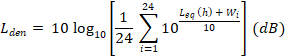
where:
Lden = Community Noise Equivalent Level in dB;
Leq(h) = equivalent sound level (see definition) for the ith hour; and
Wi = 0 for day hours (7:00 a.m. to 7:00 p.m.)
= 5 for evening hours (7:00 p.m. to 10:00 p.m.)
= 10 for night hours (10:00 p.m. to 7:00 a.m.)
The equation can also be written as follows and can be applied when the equivalent sound level is known for each part of the day:
Equation 16-2: Alternative Formula for Community Noise Equivalent Level

where:
Lden = Community Noise Equivalent Sound Level in dB;
Lday = equivalent sound level for day hours (7:00 a.m. to 7:00 p.m.)—the day term in the equation can be divided by peak and off-peak traffic hours if desired, with the appropriate constant of elapsed time/24 hours applied;
Leve = equivalent sound level for evening hours (7:00 p.m. to 10:00 p.m.); and
Lnight = equivalent sound level for night hours (10:00 p.m. to 7:00 a.m.).
The CNEL can also be expressed in terms of SEL as follows:
Equation 16-3: Formula for Community Noise Equivalent Level based on SEL

where:
LAE = SEL in dB (see definition);
Nday = Number of vehicle pass-bys between 7:00 a.m. to 7:00 p.m., local time;
Neve = Number of vehicle pass-bys between 7:00 p.m. to 10:00 p.m., local time;
Nnight = Number of vehicle pass-bys between 10:00 p.m. to 7:00 a.m., local time; and
49.4 = A normalization constant that spreads the acoustic energy associated with highway vehicle pass-bys over a 24-hour period [i.e., 10 log10 (86,400 seconds per day) = 49.4 dB].
See Noise Contamination.
DNL is a 24- hour A-weighted average sound level for a given day, after the addition of 10 dB to sound levels between the nighttime hours of 2200 (10:00 p.m.) and 0700 (7:00 a.m.) (“penalty” for sleep time). Unit, dBA (assumes A-weighting). Ldn is computed as follows based on hourly equivalent sound levels:
Equation 16-4: Formula for Day-Night Average Sound Level
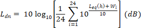
where:
Ldn = Day-Night Average Sound Level in dB;
Leq(h) = equivalent sound level (see definition) for the ith hour; and
Wi = 0 for day and evening hours (7:00 a.m. to 10:00 p.m.)
= 10 for night hours (10:00 p.m. to 7:00 a.m.)
The equation can also be written as follows and can be applied when the equivalent sound level is known for each part of the day:
Equation 16-5: Alternative Formula for Day-Night Average Sound Level
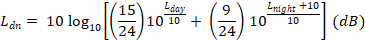
where:
Ldn = Day-Night Average Sound Level in dB;
Lday = equivalent sound level for day hours (7:00 a.m. to 10:00 p.m.)—the day term in the equation can be divided by peak and off-peak traffic hours if desired, with the appropriate constant of elapsed time/24 hours applied; and
Lnight = equivalent sound level for night hours (10:00 p.m. to 7:00 a.m.).
The day-night average sound level can also be expressed in terms of SEL as follows:
Equation 16-6: Formula for Day-Night Average Sound Level based on SEL

where:
LAE = SEL in dB (see definition);
Nday = Number of vehicle pass-bys between 7:00 a.m. to 7:00 p.m., local time;
Nnight = Number of vehicle pass-bys between 10:00 p.m. to 7:00 a.m., local time; and
49.4 = A normalization constant which spreads the acoustic energy associated with highway vehicle pass-bys over a 24-hour period [i.e., 10 log10 (86,400 seconds per day) = 49.4 dB].
A decibel is a unit of level that denotes the ratio between two quantities that are proportional to power; the number of decibels is 10 times the base 10 logarithm of this ratio. For the purpose of this document, the reference level of sound pressure or noise is 20 μPa (approximately the threshold of human hearing at 1 kHz). The reference level of vibration is 1 μ-inches/second.
A diffracted wave is a sound wave whose front has been changed in direction by an obstacle or other non-homogeneity in the propagation medium, typically air for the purposes of this document, other than by reflection or refraction.
Divergence is the spreading of sound waves from a source in a free-field environment. In the case of highway noise, two types of divergence are common: spherical and cylindrical. Spherical divergence occurs for sound emanating from a point source (e.g., a single vehicle pass-by). It is independent of frequency, and is computed using a 20 log10(d1/d2) relationship. For example, if the sound level from a point source at 50 ft (15 m) was 90 dB, then at 100 ft (30 m) it would be 84 dB due to divergence [i.e., 90 + 20 log10 (50/100)]. Cylindrical divergence occurs for sound emanating from a line source, (e.g., continuous traffic on a highway). It is independent of frequency, and is computed using a 10 log10 (d1/d2) relationship. For example, if the sound level from a line source at 50 ft (15 m) was 90 dB, then at 100 ft (30 m) it would be 87 dB due to divergence [i.e., 90 + 10 log10 (50/100)].
Dynamic range is the difference between the highest input SPL achievable without exceeding a specified nonlinearity or distortion of the output signal, for a specified frequency range, and the lowest input SPL for which the level linearity is within specified tolerances. Dynamic range is discussed further in Section 17.3.3.2.
The Equivalent Sound Level or Equivalent Continuous Sound Level (TEQ or Leq, denoted by the symbol LAeqT, or generically, Leq) is ten times the base-10 logarithm of the ratio of time-mean-squared instantaneous sound pressure, during a stated time interval, T (where T=t2-t1), to the square of the standard reference sound pressure. Unit, dBA (assumes A-weighting). For the purpose of this document, the reference sound pressure is 20 μPa. The equivalent sound level is a time-averaged sound level that has the same acoustic energy as the time-varying sound level during the same time period. LAeqT can be measured and reported for a specific time interval T or it can be calculated from multiple samples as follows:
Equation 16-7: Formula for Equivalent Sound Level

where:
LAeqT = A-weighted equivalent sound level in dB for time T;
SPL1, SPL2, …SPLN = first, second, and Nth A-weighted sound pressure level;
N = number of sound level samples; and
T = total time interval constructed from N samples
[e.g., T = 1 hour for twelve 5-minute samples; in this case the sound descriptor can be written as LAeq1h or another common format, Leq(h)].
The equivalent sound level can also be expressed in terms of SEL as follows:

where:
LAeqT = equivalent sound level in dB;
LAE = SEL in dB (see definition); and
t1, t2 = t1 is the start time, and t2 is the end time for the time interval.
The exponential time-weighted sound level is 10 times the logarithm to the base 10 of the ratio of the running time average of the exponential-time-weighted and frequency-weighted squared sound pressure to the square of the reference pressure. Unit, decibel (dB). Exponential time weightings are most commonly fast-scale (τ = 0.125 seconds) and slow-scale (τ = 1.0 seconds), where τ is the exponential time constant, which is the time required to increase the time-varying quantity by (1 – 1/e), or decrease by (1/e). Sound level fluctuations are easier to read on a sound level meter with the slow setting compared to the fast setting; however, the fast setting gives better resolution of instantaneous response. See Appendix B for a more detailed discussion of exponential time averaging.
Far field is the acoustic field sufficiently distant from a distributed source that the sound pressure decreases with the applicable geometrical divergence with increasing distance (neglecting reflections, refraction, and absorption). This occurs when the SPL (due to this sound source) decreases by 6 dB per doubling of distance from the source (i.e., spherical divergence); or if the sound source is linear, then the far field is the portion of the sound field in which the SPL decreases by 3 dB per doubling of distance.
Free field is a sound field in a homogeneous medium whose boundaries exert a negligible influence on the sound waves. In a free-field environment—absent atmospheric effects—sound spreads spherically from a source and decreases in level at a rate of 6 dB per doubling of distance from a point source, and at a rate of 3 dB per doubling of distance from a line source.
Frequency is the rate of change with time of the instantaneous phase of a sine function divided by 2π, with dimensions of cycles per second or hertz (Hz).
Ground attenuation is the change in sound level—either positive or negative—due to intervening ground between source and receiver. Ground attenuation is a relatively complex acoustic phenomenon, which is a function of ground characteristics, source-to-receiver geometry, and the spectral characteristics of the source. A commonly used rule-of-thumb for propagation over soft ground (i.e., grass, terrain) is that ground effects will account for about 1.5 dB per doubling of distance (in addition to divergence). However, this relationship is quite empirical and tends to break down for distances greater than about 100 ft to 200 ft (30 m to 61 m). Specific methodologies have been developed to estimate ground attenuation, such as that utilized in FHWA’s Traffic Noise Model.
Ground impedance is a complex function of frequency relating the sound transmission characteristics of a ground surface type. Measurements to determine ground impedance can be made in accordance with ANSI/ASA S1.18-2010.[85]
Hard ground, also referred to as acoustically hard ground, is any highly acoustically reflective surface in which the phase of the sound energy is essentially preserved upon reflection. Examples include water, water-soaked earth, hard-packed earth, asphalt, and concrete. Although the effects of hard ground vary by frequency, the overall result is a net amplification in sound (reflected sound adds to direct sound).
Insertion loss is the difference in levels BEFORE and AFTER installation of a barrier (encompassing all causes of the difference), where the source, terrain, ground, and atmospheric conditions, in the BEFORE and AFTER cases, are equivalent.
kHz is an abbreviation for 1,000 hertz (Hz); hertz is a unit of frequency.
See Sound Exposure Level (SEL, denoted by the symbol LAE).
See Equivalent Sound Level or Equivalent Continuous Sound Level.
See Maximum Sound Level (MXFA or MXSA, denoted by the symbol LAFmx or LASmx, respectively).
See Community Noise Equivalent Level (CNEL, denoted by the symbol Lden).
See Day-Night Average Sound Level (DNL, denoted by the symbol Ldn).
L90 is a statistical descriptor describing the sound level exceeded 90% of a measurement period. Unit, dBA (assumes A-weighting).
A line source is multiple closely spaced or moving point sources collectively radiating sound cylindrically. (Sound levels measured from a line source decrease at a rate of 3 dB per doubling of distance in free-field conditions.)
Lower bound to insertion loss is the value reported for insertion loss when background levels are not measured or are too high to determine the full attenuation potential of the barrier.
Maximum sound level is the maximum, A-weighted and exponential-time-weighted (fast or slow) sound level associated with a given event or during a time interval (Figure 16-1). Unit, dBA (assumes A-weighting).
Near field is the acoustic field so close to an extended source that the effects of the source size are manifest in the measurements. The near field is between the source and the far field. The near field exists under optimal conditions at distances less than four times the largest sound source dimension.
Noise is any unwanted sound. Objectively, noise can be defined as erratic, intermittent, or statistically random oscillation (variation from reference).
A noise barrier is a wall or earth berm (or combination of the two) that interferes with sound propagation and minimizes excessive or intrusive noise for inhabitants of noise-sensitive land uses near a noise source (e.g., busy highway).
Noise contamination is any noise event other than that which is intended for measurement. Contamination typically occurs when the background noise is within 10 dB of the noise produced by the source intended for measurement.
Noise reduction coefficient is the single-number rating of the sound absorption properties of a material; it is the arithmetic mean of the Sound Absorption Coefficient at 250 Hz, 500 Hz, 1,000 Hz, and 2,000 Hz, rounded to the nearest multiple of 0.05 metric sabins per square meter. Measurements to obtain the noise reduction coefficient value are performed in accordance with ASTM Standard C423.
Octave bands are sounds that can be represented by several frequency bands between two frequency limits (for human hearing the frequency limits are 20 Hz to 20,000 Hz). One customary bandwidth is one octave, where the upper frequency limit of the band is approximately twice (21/1) the lower limit. Octave bands are represented by their center frequencies (e.g., 31.5 Hz, 63 Hz, 125 Hz, 250 Hz, 500 Hz, and 1,000 Hz).
One-third octave band is the most customary bandwidth for a highway noise frequency analysis. One-third octave bands reveal more details in the spectral content than octave bands and are typically appropriate for highway traffic noise. The upper frequency limit for a one-third octave band is approximately 1.26 (21/3) times the lower limit. One-third octave bands are represented by their center frequencies (e.g., 20 Hz, 25 Hz, 31.5 Hz, 40 Hz, 50 Hz, 63 Hz, 80 Hz, 100 Hz, 125 Hz, 160 Hz, 200 Hz, 250 Hz, 315 Hz, 400 Hz, 500 Hz, 630 Hz, 800 Hz, and 1,000 Hz).
Peak sound level is the peak, A-weighted sound level associated with a given event or during a time interval. This is based on the peak [as opposed to root-mean-squared (RMS)] instantaneous sound pressure. Unit, dBA (assumes A-weighting). The peak sound level is often used to assess hearing damage from impulsive noises and is rarely applied to environmental noise measurements. See also Maximum Sound Level (MXFA or MXSA, denoted by the symbol LAFmx or LASmx, respectively).
Peak particle velocity is the maximum instantaneous positive or negative peak of the vibration signal. Unit, micro-inches/second.
Pink noise is a random or pseudorandom signal intended to have equal energy in each octave or one-third octave band. (Pink noise generators are sometimes used to check signal quality prior to noise measurements.)
Point source is a source that radiates sound spherically. (Sound levels measured from a point-source decrease at a rate of 6 dB per doubling of distance in free-field conditions.)
Sabine absorption coefficient is the absorption coefficient obtained in a reverberation room by measuring the time rate of decay of the sound energy density with and without a patch of the sound-absorbing material under test laid on the floor. These measurements are performed in accordance with the ASTM Standard C423. Unit, metric sabins per square meter.
Soft ground, which is also referred to as acoustically soft ground or porous ground, is any highly absorptive surface in which the phase of the sound energy is changed upon reflection, except at low frequencies. Examples include grassland, terrain covered with dense vegetation, plowed or aerated earth, or freshly fallen snow. Although the effects of soft ground vary by frequency, for sound propagation angles typically associated with highway traffic noise, the overall result is an attenuation in reflected noise as compared to hard ground. (At propagation angles greater than 20° from horizontal, which can occur at short ranges, or in the case of elevated sources or receivers, soft ground becomes a good reflector and can be considered hard ground.) See also Ground Attenuation and Hard Ground.
Sound absorption coefficient is the ratio of the sound energy, as a function of frequency, absorbed by a surface, to the sound energy incident upon that surface. See also Sabine Absorption Coefficient.
Sound exposure level is 10 times the logarithm to the base 10 of the ratio of a given time integral of squared instantaneous sound pressure to the squared reference sound pressure of 20 μ Pa. Unit, dBA (assumes A-weighting). The time interval must be long enough to include most of the sound source’s acoustic energy. At a minimum, this interval should encompass the 10 dB down points (Figure 16-1).
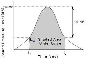
In addition, LAE is related to LAeqT by the following equation:

where:
LAE = Sound exposure level;
LAeqT = Equivalent sound level in dB (see definition above); and
t1, t2 = t1 is the start time, and t2 is the end time for the time interval.
Sound intensity is the average rate of sound energy transmitted in a specified direction at a point through a unit area normal to this direction at the point considered. Unit, watt per square meter (power/area) [W/m2= N/(s*m)]. Since sound intensity is sound power over an area, it is dependent on the shape of the sound wave. For example, for a spherical wave, area = 4πr2, where r is the distance from the sound source at which intensity is being evaluated. Sound intensity is directly proportional to the square of prms (RMS pressure) and is related by the density (ρ) and speed of sound (c) in a medium: I = (prms)2/(ρ*c).
Sound intensity level is 10 times the base-10 logarithm of the ratio of a time-average intensity of a given sound in a stated direction, to the reference value for sound intensity of 1 picowatt per square meter (picoW/m2). Unit, dBA (assumes A-weighting). Sound intensity level values can apply to broadband levels or for a stated frequency band.
Sound power, for a specified sound source, is the sound energy radiated per unit of time (rate of energy flow). Unit, watt (W = J/s = N*m/s).
Sound pressure is the total instantaneous pressure at a point in a medium minus the static pressure at that point. Unit, pascal (Pa = N/m2). Sound pressure (prms) squared is directly proportional to sound intensity and is related by the density (ρ) and speed of sound (c) in a medium: (prms)2 = I*(ρ*c). Since sound intensity is related to sound power, sound pressure is also related to sound power.
Sound pressure level is 10 times the base-10 logarithm of the ratio of the square of prms (RMS pressure) signal, to the square of the reference sound pressure of 20 μPa, the approximate threshold of human hearing at 1 kHz. Unit, dBA (assumes A-weighting). SPL values can apply to broadband levels or for a stated frequency band.
Sound transmission class is a single-number rating used to compare the sound insulation properties of barriers, including windows and doors in buildings.
Spectrum is a signal’s resolution expressed in component frequencies or fractional octave bands.
This section describes field measurement instrumentation for sound, vibration, and other measurement systems.
A microphone transforms sound pressure variations into electrical signals that are measured by sound level meters or one-third octave band spectrum analyzers. These electrical signals are also often recorded digitally for later off-line analysis. Microphone characteristics are further addressed in ANSI/ASA S1.4-2014/Part 1.[86]
A preamplifier provides high-input impedance and constant, low-noise amplification over a wide frequency range.[87] Also, depending on the type of microphone being used (Section 17.1.1.1), a preamplifier may also provide a polarization voltage to the microphone. The manufacturer typically provides paired microphone-preamplifier units.
Use a tripod or similar device to support the microphone system (microphone and preamplifier). Isolate the microphone system from the support, especially if the support is made up of a metal composite. In certain environments, the support can act as an antenna, picking up errant radio frequency interference that can potentially contaminate data. Common isolation methods include encapsulating the microphone system in nonconductive material (e.g., nylon) prior to fastening it to the support.
Observe the correct grazing incidence (Section 17.1.1.3) when attaching a microphone/sound level meter system to a tripod. In addition, ensure that the microphone system is positioned relative to the support device to minimize contamination due to sound reflections from the support. Research has shown that a position directly behind the support device provides for minimum interference.[88]
Once supported appropriately, position the microphone as appropriate for the type of measurement. Connect the microphone system to the measuring/recording instrumentation via an extension cable using at least 50 ft (15 m) of cable; this minimizes any potential contamination of the measured data due to operator activity.
Condenser (or electrostatic or capacitor) microphones are recommended for several measurement purposes because of their high stability, reasonably high sensitivity, excellent response at high frequencies, and low electrical noise characteristics. Pre-polarized condenser microphones are commonly used with modern sound level meters. There are two types of condenser microphones: conventional and electret.
Conventional condenser microphones characterize magnitude changes in sound pressure in terms of variations in electrical capacitance. Changes in sound pressure move the diaphragm and change the spacing between the diaphragm and the microphone backplate. This dynamic change in the gap between the diaphragm and backplate translates to a change in electrical capacitance. In the case of a conventional condenser microphone, a polarization voltage must be applied to the backplate. Typically, the preamplifier applies a polarization voltage between 50 V and 200 V to the microphone backplate. Due to the requirement that a polarization voltage be supplied from a source external to the microphone (i.e., the microphone is not a “closed” system), measurements made with a conventional condenser microphone are often adversely affected by atmospheric conditions, especially high humidity. High humidity can result in condensation between the microphone diaphragm and backplate. Condensation can cause arcing of the polarization voltage, rendering the measured data essentially useless.[89],[90] Use of dehumidifying chambers, desiccants, and nonconductive back coating, such as quartz to minimize condensation effects. Several manufacturers provide devices to minimize this often-overlooked potential problem.
As opposed to conventional condenser microphones, electret condenser microphones use a thin plastic sheet with a conductive coating on one side as a backplate. This design allows the microphone to maintain its own polarization (i.e., often referred to as a “pre-polarized” design).[91] “Pre-polarization” allows the electret microphone to be essentially a “closed” system, eliminating the potential for condensation in high-humidity environments.
The diameter of a microphone diaphragm directly affects its usable frequency range, dynamic range (or level sensitivity), and directivity. For example, as the microphone diameter becomes smaller, the useable frequency range increases; however, sensitivity decreases.89,[92] Thus, the selection of a microphone size often involves a compromise of these elements. Unless measurements at extremely low SPLs are required (e.g., below 20 dB SPL) a 0.5 in. (1.27 cm) diameter microphone is suitable for most situations. For low-SPL measurements, a 1-in. diameter microphone may be necessary, although some 0.5-in. microphones are capable of low-SPL measurements.
Microphone sensitivity varies with the angle of incidence between the sound waves and the microphone diaphragm. Two microphone system orientations and their specific applications are discussed below: normal and grazing incidence.
Normal incidence, also referred to as 0° incidence, occurs when sound waves impinge at an angle perpendicular, or normal, to the microphone diaphragm (Figure 17-1). Normal incidence is best used for situations involving point-source measurements, in which the sound being measured is coming from a stationary, single, known direction (e.g., an idling automobile or a power generator).
Grazing incidence systems, also referred to as 90° incidence, occurs when sound waves impinge at an angle that is parallel to, or grazing, the plane of the microphone diaphragm (Figure 17-1). This orientation is preferred for moving—or line-source—measurements since the microphone presents a constant incidence angle to any source located within the plane of the microphone diaphragm.
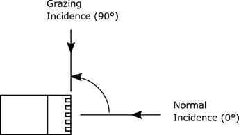
Grazing incidence is commonly used for the measurement of highway, aircraft, and guided-transit noise. Correction of the measured data in accordance with manufacturer-published response curves is required if other than grazing incidence is used for the measurement of moving noise sources. This process can be quite complex because the incidence angle is continually changing, thus requiring continuously varying corrections. It is perfectly acceptable to position a microphone for grazing incidence even if it has its flattest frequency response characteristics in a normal incidence configuration if the appropriate manufacturer-published corrections are applied, and if the required corrections do not exceed certain limits.[93] If the manufacturer does not provide the appropriate incidence corrections, then perform tests in accordance with ANSI/ASA S1.10-1986 (R2001).[94]
Base microphone corrections on random-incidence response curves when measuring randomly occurring sounds (e.g., background noise measurements, or existing noise measurements where the location of the sound source can be arbitrary).
There are two types of transducers used to measure groundborne vibration: geophones and accelerometers. Both types of transducers convert the vibratory motion of the sensor to an electrical signal. Vibration transducers may not require a preamp, in contrast with microphones (e.g., most geophones produce an electrical signal that is suitable for recording directly). Both types of devices are small and mounted directly to the ground. Vibration transducers may be attached to a spike or ground stake for good coupling when used in soil. For attaching to hard surfaces, transducers can be adhered using epoxy, museum wax, or earthquake gel. Vibration transducers must have a vertical vibration measurement component. Many transducers include triaxial units that measure vertically and horizontally in two directions. Only vertical vibration measurements are described herein.
Geophones measure the velocity of vibration of the ground. Geophones comprise a mass in a coil magnet. Movement of the mass creates voltage in the coil that is proportional to the velocity of the mass. Geophones are limited by their frequency range. The construction and design of the geophone results in the system having a typical natural frequency, below which the signal rolls off. Common geophones have a natural frequency of 10 Hz. Some geophones have natural frequencies of 2 Hz or even 1 Hz. It may be acceptable to apply a correction to the low frequency data to account for the roll-off below the natural frequency. Use accelerometers if low frequency data is a primary concern of measurements.
Accelerometers also comprise a mass that creates an electrical signal as it moves. The electrical signal is proportional to the acceleration of the mass. Commonly used seismic accelerometers use piezoelectric crystals. As the mass moves, the movement compresses the crystal and varies the charge across the crystal faces. Accelerometers may also be made from capacitive systems or microelectromechanical systems. Accelerometers typically have wide frequency ranges, from 1 Hz to several kilohertz. Many accelerometers also measure static (or 0 Hz) acceleration, though these are not often used for measuring vibration.
A waveform recorder directly captures the input signal from an acoustical or vibration transducer. There are two basic types of recorders: analog and digital. Analog recorders store signals as continuous variations in the magnetic state of the particles on the tape. Digital recorders store signals as a combination of binary “1s”and “0s.” Most digital recorders represent a continually varying analog level using many discrete 16- or 24-bit words (i.e., a unique combination of 16 or 24 “1s”and “0s”). The number of 16-bit words depends on the recorder’s sampling rate. The sampling rate must be at least twice the highest frequency of interest, which is often 20 kHz for transportation-related measurements. In theory, this means that one second of continuously varying analog data is represented by at least 40,000 discrete samples. However, in practice—and due to the design limitations on anti-alias filters (anti-alias filters are described)—a sampling rate of 44,000 to 48,000 is common (i.e., 44,000 to 48,000 discrete 16-bit combinations of “1s”and “0s”) (Section 17.3.3.1). Not all field measurement systems will include a recorder. A recorder offers the unique capability of repeated playback of the measured noise source, allowing for more detailed analyses. The advantages of modern digital over analog recorders are numerous. Digital recorders typically have much wider frequency response characteristics, and a much larger dynamic range.
Sound level meters and sound level analyzers measure sound levels. Section 772.11(d) (3) of 23 CFR 772 calls for the use of an integrating sound level meter or analyzer, which automatically measures Leq. Sound level meters (SLMs) should perform true numeric integration and averaging in accordance with ANSI/ASA S1.4-2014/Part 1.[95] Components of an SLM include (Figure 17-2): a microphone with preamplifier, an amplifier, frequency weighting, input gain control, time averaging, and an output indicator or display. Base selection of a specific model of sound level meter on cost and the level of accuracy desired, input gain control, time averaging, and an output indicator or display.
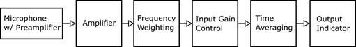
The accuracy of an SLM is characterized by its “class.” There are three types of SLMs available: class 0, 1, and 2. Class 0 SLMs are designed for laboratory reference purposes, where the highest precision is required. Class 1 SLMs are designed for precision field measurements and research. Either class 1 or class 2 SLMs are acceptable for use in traffic noise analyses for Federal-aid highway projects.
An analyzer has automated sampling features that a meter generally does not have. Additionally, many sound level analyzers will also automatically compute the “exceedance” statistics such as L10, L50, and L90. Analyzers can usually sample and store results for multiple intervals—typically ranging from one second to an hour—within a longer-duration measurement. Having the measurement data broken into short intervals allows “bad” (contaminated or unrepresentative) data to be eliminated without losing an entire measurement. The length of the intervals will depend on the amount of data storage on the device. The practitioner should select the shortest interval setting that still allows data to be recorded for the full measurement period.
Employ a one-third octave band analyzer when the frequency characteristics of the sound source are of concern. Employ these units to determine noise spectra and compute various noise descriptors, such as LAeqT and LAE. One-third octave band filters must be shown to comply with a Type 1-D Butterworth filter, as defined in ANSI/ASA S1.11-2014.[96] The Type 1-D Butterworth filter design has existed in analyzers for decades. However, manufacturers are now providing filter-shape algorithms that depart from the traditional Butterworth design, and more closely resemble “ideal” filters, which allow essentially no energy outside of the pass-band.
There are several important issues or differences to consider when selecting a specific model of recorder or sound level meter.
The bandwidth of a measurement instrument refers to its frequency range of operation. Most measurement instrumentation will accurately measure levels in the frequency range 20 Hz to 20 kHz, the audible range for humans. Typically, measurement of one-third octave band data between 50 Hz and 10 kHz will satisfy the objectives of highway-related noise studies.
The bandwidth for vibration is considerably lower than for noise. The ISO publication Mechanical vibration and shock – Evaluation of human exposure to whole-body vibration (ISO 2631) indicates that humans are sensitive to vibration in the range of 8 Hz to 80 Hz. Likewise, FTA’s Transit Noise and Vibration Impact Assessment[97] defines criteria for vibration in the range of 8 Hz to 80 Hz. Structures and sensitive equipment may be sensitive to vibration as low as 1 Hz. Vibration at frequencies higher than 80 Hz can also contribute to groundborne noise. Therefore, humans may be sensitive to frequencies as high as 160 Hz or 200 Hz. When measuring vibration, the measurement system must have a minimum bandwidth of 1 Hz to 80 Hz. Vibration frequencies as high as the 315 Hz one-third octave band are often collected, particularly if groundborne noise is of concern.
The bandwidth for digital recorders is defined by their sampling frequency. As described, the sampling frequency represents the number of times per second that the input signal from a transducer is captured by the recording system. The signal must be sampled at double the maximum frequency of interest, and the sampling frequency is typically somewhat higher than this, in part due to the need for anti-alias filters. An anti-alias filter is a low-pass filter applied to the input signal of a digital system prior to the digitization process. This filter, unique to digital systems, ensures that spurious signals (alias signals) resulting from the digitization process are not contributing components of the sampled signal. An anti-alias filter must have attenuation characteristics, which reduces the contribution of aliased frequency components in the output to a negligible level.[98]The system’s digitization process and the on-board electrical filters govern the bandwidth for SLMs. Because SLMs are specifically designed for measuring acoustic signals, the bandwidth is typically 20 Hz to 20 kHz.
Digital recorders can record frequencies as low as 0 Hz, whereas SLMs often do not measure below 16 Hz or 20 Hz. When measuring vibration, ensure that the bandwidth includes low frequencies (down to 1 Hz). Some SLMs have factory settings available that enable low-frequency measurement.
Dynamic range is the difference in decibels between the maximum and minimum levels measured by a recording system. The measurement system should have a dynamic range wide enough that the highest levels measured do not overload the system and the lowest levels measured are sufficiently above the system noise floor to avoid contamination. As individual sensors have a dynamic range (Microphone Size), so too does the complete system.
The dynamic range is defined by the interaction of all components of the measurement system, including transducer, cabling, connections, amplification, digitization, electronics, and recording. The maximum level may be limited by elements such as the physical design of the transducer or the voltage input limits to the data recorder. The minimum level is likewise limited by elements such as the physical properties of the transducer, noise introduced at the cabling or amplification stage, or the analog-to-digital conversion bit depth.
The digitization process often controls the dynamic range at both the upper and lower limits. The overload point in a digital system is a well-defined point controlled by the maximum size of the bit-register used in the digitization process. When the size of the bit-register is exceeded, “hard” limiting occurs, followed by instantaneous distortion. In most cases, the upper limit of the dynamic range of a digital recorder is specified from this “hard” limiting point, and the overload and full-scale indicators are referenced to it. In contrast, analog recorders have no clearly defined overload point and generally “soft” limiting (a gradual process) begins around 6 dB above the full scale (0 dB) on a volume unit meter, with the subsequent gradual increase in distortion. The lower limit of the system is also controlled by the analog-to-digital converter. As there is a maximum bit size, there is also a minimum bit size. Signal levels below this bit value are not detected and not recorded.
Sixteen-bit digital recorders have a total dynamic range approximately 80 dB, while 24-bit recorders are approximately 100 dB. In contrast, many microphones will have a full dynamic range greater than 130 dB. The dynamic range of the transducer should be compared to that of the data recorder. Manufactures typically provide microphone/sound level meter pairs that are compatible with each other.
Many recorders and SLMs offer options to adjust the input range or gain. Adjust the input gain of a measurement system to provide for maximum dynamic range while preserving a modest safety factor to avoid overload. To avoid system overload, set the gain so that the expected maximum level of the source being measured is 20 dB below overload. Increasing the maximum level can also raise the noise floor. It is recommended that the linear operating range of the measurement system is in accordance with tolerances specified in IEC 61265:1995,[99] a standard specific to aircraft noise measurement.
Frequency weighting accounts for changes in sensitivity of the human ear as a function of frequency. Three standard weighting networks—A, B, and C—account for different responses to SPLs (Figure 17-3 and Table 17-1). (The absence of frequency weighting is referred to as “flat” response.)
C-weighting is essentially linear, although there are small adjustments at frequencies below 40 Hz and above 8000 Hz. B-weighting reflects the human ear’s response to sounds of moderate pressure level. A-weighting reflects the human ear’s response to sounds of lower pressure level.[100] A-weighting is the most widely used system for assessing transportation-related noise. In fact, unless otherwise stated, noise descriptors for transportation-related activity are assumed to be A-weighted. Most SLMs and one-third octave band analyzers offer A- and C-weighting options. B-weighting is obsolete. (The response for the A-, B-, and C- weighting curves are all referenced to a frequency of kHz. In other words, the weighting at 1 kHz for all three curves is zero.)
Modern SLMs also include a Z-weighting. The Z-weighting is flat between 10 Hz and 20 kHz, as opposed to the C-weighting, which rolls off high and low frequencies. (Vibration measurements are not weighted and should use a Z-weighting or unweighted option.)
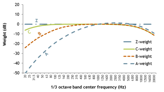
Exponential time averaging is a method of stabilizing instrumentation response to signals with changing amplitudes over time using a low-pass filter with a known, electrical time constant. The time constant is defined as the time required for the output level to reach 67% of the input, assuming a step-function input. Also, the output level will typically reach 100% of an input step-function after approximately five time constants. The exponential time-averaged output produced by the low-pass filter is a running average dominated by the most recent value but smoothed out by the contribution of the preceding values. Two exponential time-averaging response settings are used for traffic and environmental noise: fast and slow, with time constants (J) of 0.125 second and 1 second, respectively (Figure 17-4).

Slow response is typically used for measurements of sound source levels that vary slowly as a function of time, such as aircraft. Fast response is typically used for measuring individual highway vehicle pass-bys (Section 10.0). Slow response is recommended for the measurement of long-term effects due to highway noise, where impulsive noises are not dominant.
Temperature and humidity can affect the sensitivity of many types of instrumentation, including microphones and spectrum analyzers. As discussed in Section 17.1.1, non-electret condenser microphones are subject to arcing under high-humidity conditions. Also, battery life is substantially shortened when subject to prolonged low temperatures. Follow manufacturers’ recommendations for acceptable temperature and humidity ranges for equipment operation. Typically, recommendations range from -10°C to 50°C (14°F to 122°F) and from 5% to 90% relative humidity.
Data storage is an important element of any analog or digital system. Analog systems use magnetic tape to store information, which is delicate and bulky. Modern digital systems use solid-state memory, which is physically small relative to the total device size. Digital memory for field measurement systems can be as high as tens or hundreds of gigabytes (GB). Waveforms recorded at 24-bit resolution and sampling frequencies of 40,000 samples per second can require significant memory; nevertheless, it is still frequently possible to record several hours—or even days—worth of data using a single recording device. Sound level meters do not typically record waveforms; rather, these meters store processed data in the form of Leq or other noise descriptors. This offers tremendous savings for memory; consider a single 1-second Leq value stored compared to 40,000 values stored for a waveform for that second. Because of this, SLMs are sometimes manufactured with limited storage capabilities to save costs. Most modern digital devices offer easy and fast download of data to computers, either by physically connecting the device to a computer with a data transfer cable, or by allowing removal of the storage media. If the digital storage is not sufficient to complete field measurements, then transfer the data to a laptop or hard-drive in the field and remove the data from the SLM. Consult manufacturers for information about data storage and transfer.
An acoustic calibrator provides a means of checking the entire acoustic instrumentation system’s (i.e., microphone, cables, and recording instrumentation) sensitivity by producing a known SPL (referred to as the calibrator’s reference level) at a known frequency, typically 94 dB or 114 dB at 1 kHz, or 124 dB at 250 Hz. The calibrator used for measurements described herein should meet the Type 1L performance requirements of IEC 60942:2003.[101] Calibrate acoustic instrumentation at the beginning and end of each measurement session, and BEFORE and AFTER any changes are made to system configuration or components. Use the following procedure to determine calibration (CAL) adjustments prior to data analysis:
CAL adjustment = Reference level - [(CALINITIAL + CALFINAL) / 2]
For example, if:
Reference level (manufacturer’s calibration level) = 114.0 dB
Initial calibration level = 114.0 dB
Final calibration level = 114.4 dB
Then:
CAL adjustment = 114.0 - [(114.0 + 114.4)/2] = -0.2 dB
In this example, adjust the measured Leq downward by 0.2 dB, with a note that it has been adjusted.
In accordance with ANSI/ASA S1.13-2005,[102] establish the electronic noise floor of the entire acoustic instrumentation system on a daily basis by substituting the measurement microphone with a passive microphone simulator (dummy microphone) and recording the noise floor for a period of at least 30 seconds. A dummy microphone electrically simulates the actual microphone by providing a known fixed (i.e., passive) capacitance that is equivalent to the minimum capacitance the microphone can provide. This permits valid measurement of the system’s electronic noise floor.
With the microphone removed and the simulator inserted in its place, monitor all input channels of the instrumentation system using headphones. Extraneous signals, such as radio interference or hum, can result when the system is located near antennae, power lines, transformers, or power generators. The system is especially susceptible to such interference when using long cables that essentially act as antennae for such signals. Eliminate extraneous signals or reduce these signals to a negligible level (i.e., at least 40 dB below the expected maximum level of the measured noise source). This can usually be accomplished by reorienting the instrumentation or cables, using shorter cables, checking and cleaning grounding contacts, or—in a worst-case scenario—moving the instrumentation system away from the source of the interference, if the position of the source is known.
Establish the frequency response characteristics of the entire acoustic instrumentation system on a daily basis by measuring and storing 30 seconds of pink noise. Pink noise is a random signal for which the spectrum density (i.e., narrow-band signal) varies as the inverse of frequency. In other words, one-third octave band spectral analysis of pink noise yields a flat response across all frequency bands.
Place windscreens atop all microphones used in outdoor measurements. A windscreen is a porous sphere placed atop a microphone to reduce the effects of wind-generated noise on the microphone diaphragm. The windscreen (preferably new) should be clean, dry, and in good condition. Typically, the effect on the measured sound level due to the insertion of a windscreen into an acoustic instrumentation system can be neglected. The windscreen manufacturer should provide a table of corrections based on frequency and angle of interest. Conduct tests for high-precision measurements in an anechoic chamber if a manufacturer does not provide corrections.
Weather data should be site-specific and contemporaneous with the sound level measurements. Properly document meteorological conditions, especially wind speed and direction, which can affect measured noise levels near a highway. This effect typically increases in magnitude with increasing distance from the source. Other factors that can affect sound include temperature, humidity, and barometric pressure. Many handheld weather measurement units can record all four of these parameters.
Research has shown that wind speed and direction may affect measured noise levels near a highway.[103] These effects typically increase with increasing distance from the noise source. An anemometer is an instrument that measures wind speed. Anemometers should meet the requirements of ANSI/ASA S12.18-1998 (R2009).[104]
For general-purpose measurements at relatively close distances to a noise source (i.e., within 100 ft (30 m), a handheld, wind-cup anemometer and an empirically observed estimation of wind direction are sufficient to document wind conditions. For research purposes or for measurements where the receiver(s) will be positioned at distances greater than 100 ft (30 m) from the noise source, use a high-precision anemometer, capable of measuring wind conditions in three dimensions, integrated into an automated, data-logging weather station. For all types of measurements, position the anemometer at a relatively exposed position and at an elevation approximately equal to that of the highest receiver position.[105]
Wind can flutter the microphone diaphragm and produce false noise readings (even through a proper windscreen). Sound level measurements made during winds exceeding 11 mph (17 kmh or 5 m/s) may be contaminated. If the A-weighted sound levels are lower than 40 dBA, then even lower-speed winds can generate false noise. Also, wind conditions are critical in judging data equivalency; refer to Section 9.1.1.2 for details on classes of wind conditions and Section 4.4.1 for their effects on sound levels.
Temperature and humidity can affect measured sound levels, typically to a lesser degree than wind. Use a thermometer for measuring ambient temperature and a hygrometer for measuring relative humidity in conjunction with all noise measurement studies. An alternative is to use a psychrometer, which is capable of measuring both dry and wet bulb temperature. Dry and wet bulb temperatures are used to compute relative humidity (Appendix A). Use a sling psychrometer for general-purpose measurements. Use a high-precision system, such as an automated, fast-response, data-logging weather station, if for research purposes. The thermometer or other temperature sensor should have an accuracy of ±5 percent or better at full scale. Shield all temperature sensors from direct solar radiation. In addition, measuring temperature profiles may require a variable-height support device.[106] In the case where the noise source is on pavement, such as vehicle emissions (Section 10.0), practitioners should only conduct measurements when pavement is dry; emission levels may be influenced by up to 2 dB by moisture on road surfaces.[107] In addition, atmospheric absorption can substantially reduce measured sound levels, especially at high frequencies in a low-temperature, low-humidity environment. As such, use caution when comparing measured data taken under substantially different temperature and humidity conditions, especially when the distance from source to receiver is quite large, or when the sound source is dominated primarily by higher frequencies. (Refer to Section 4.4.1 for more information on judging data equivalency in terms of temperature conditions.) It is difficult to provide general rules-of-thumb, or guidance for quantifying atmospheric absorption, because of the many parameters involved; however, there are several standards that provide algorithms for computing such effects, including SAE 866A[108], ANSI/ASA S1.26-1995[109], and ISO 9613-1.[110]
Measured sound levels of transportation-related vehicles are a direct function of vehicle speed. This section discusses various instruments for measuring vehicle speed.
A Doppler-radar gun can measure vehicle speed. When using a radar gun, position it at least 400 ft (120 m) upstream of traffic flow, relative to the noise measurement microphone, and direct it toward the vehicles as they approach the microphone. This placement minimizes effects on traffic flow resulting from driver curiosity.[111] Position the radar gun 30 ft (10 m) from the centerline of the path of the measured vehicle. This will ensure that the angle subtended by the axis of the radar antenna and the direction of travel of the vehicle will be less than 5°, when the vehicle is at the microphone pass-by point. The resulting uncertainty in vehicle-speed readings, due to angular effects on Doppler accuracy, will not exceed 0.28 mph (0.5 kmh) over a speed range from 10 mph to 70 mph (15 kmh to 110 kmh).[112] In addition, some manufacturers now offer speed guns that use laser technology. Such units would also be better for determining individual vehicle speed. A radar gun will measure the largest reflective object. If there are other larger vehicles present, then it may capture those. Laser-based systems are easier to direct at a single object.
Use a stopwatch to determine vehicle speed. Position cones or observers at known distances from one another along the roadway. Maintain a separation distance of at least 50 ft (15 m). Start/stop the stopwatch at the instants the vehicle reaches the pass-by points. Determine the vehicle’s speed by dividing the distance by the measured time. It is also possible to measure vehicle speed using a video camera in conjunction with a time-synchronized display.
Light sensors can also determine vehicle speed. Position the light sensors at known distances from one another along the roadway. Maintain a separation distance of at least 50 ft (15 m). The light sensors are triggered when the vehicle reaches the pass-by points. The triggering of the sensors typically results in a signal being sent to some type of electronic detector, which in turn is programmed to read and store time of day, or compute elapsed time between pulses from a computer or other time base. Light sensor systems are commercially available at most electronics stores. The signal detector system can also trigger the start and stop of acoustic data collection.
Position pneumatic lines at known locations from one another along the roadway to determine vehicle speed. The pressure in the pneumatic line increases when a vehicle passes over it, causing a mechanical switch to close. The vehicle’s speed is determined by dividing the known distance by the measured time period. Mechanical switches can also trigger the start and stop of acoustic data collection. Be aware that noise is generated when vehicles pass over the pneumatic lines, so provide adequate distance between the pneumatic lines any sound level meter.
Many transportation-related measurements require the collection of traffic data. The type of data includes vehicle types as defined in Section 4.5.1, vehicle volumes by type, and average vehicle speed. This data may be required for: 1) determination of site equivalence; or 2) input into a highway traffic noise prediction model; see Sections 4.0 and 9.0. This section discusses various instruments for the counting and classification of roadway traffic, including the use of a video camera, counting board, or pneumatic line. If none of these instruments is available, then employ meticulous pencil/paper tabulation.
Use a video camera to record traffic in the field and perform counts off-line later. This approach, however, requires strict time synchronization between the acoustic instrumentation and the camera.
A counting board is a board with three or more incrementing devices, depending on the number of vehicle types. Each device is manually triggered to increment for a given type of vehicle pass-by. These devices can be mechanical or electronic.
A pneumatic line can be used to determine traffic counts. The pressure in the line increases when a vehicle passes over it, causing a mechanical switch to close. The mechanical switch triggers an internal counting mechanism to increment. Pneumatic lines do not record the specific vehicle mix (i.e., automobiles, trucks, and other vehicle types).
A tachometer indicates or measures the revolutions per minute of a revolving shaft. A tachometer can more completely characterize noise sources, primarily for research. A tachometer may also measure special equipment (e.g., power generators).
A fixed, artificial noise source—such as a loudspeaker—replaces an actual noise source, usually when the actual source is not available, such as might be the case for building noise-reduction measurements (Section 6.0). Where measurements using a loudspeaker source are to be directly compared with measurements made using the actual noise source, employ a high-powered omnidirectional loudspeaker system to properly simulate the direct and reflected sounds of the source.[113] The loudspeaker should produce signals of random noise filtered in one-third octave bands. Loudspeaker directional characteristics should be such that at 2,000 Hz, the free-field radiated signal out to an angle of 45° drops no more than 6 dB relative to the on-axis signal. In addition, the loudspeaker should supply sufficient output for measurements within the 80 Hz to 5,000 Hz band range.[114]
In accordance with ANSI/ASA S1.25-1991[115] and OSHA, a noise dosimeter is a small device that integrates sound pressure over time to determine a subject’s noise dose, as a percentage of a manually set maximum criterion determined by OSHA.[116] Similar to a sound level meter, components of a noise dosimeter include: a microphone with preamplifier, an amplifier, A-weighting, a squaring device, slow exponential time averaging, an exchange rate of 5 dB, and an output indicator or display.
Ensure that all support instrumentation is compatible with the acoustic instrumentation. For example, headphones should have an input impedance suitable for the recording instrumentation’s output impedance. In addition, for maximum power transfer and minimum distortion, cables used with this equipment should have a matching impedance. Finally, always make available sufficient back-up equipment (e.g., batteries, chargers, data sheets, digital storage media). There are several tools and accessories that can make data collection easier. General-use tools (e.g., screwdrivers, wrenches, and voltmeters) are useful for troubleshooting. Personal protective equipment beyond the minimum safety requirements is also often useful. Other useful accessories include the following:
The documentation for a noise study depends on the nature of the study and the planned use of the results.
For a proposed Type I highway project, a noise study report is typically prepared and includes a summary and discussion of the noise measurement results. The noise study report may have one or more appendices with detailed sound level measurement data, site photographs, meteorological and traffic count data, and copies of field logs. Some project sponsors may require a separate noise measurement report instead of an appendix to the noise study report. For some Type I highway projects, an environmental document (environmental impact statement or environmental assessment) is prepared and includes one or more sections summarizing the noise study results. These results typically include a summary of the measured sound level data and a discussion of their use for either establishing the existing noise environment or validating the FHWA TNM. Exact reporting requirements and format will vary by project sponsor, with some being more specific and prescriptive than others.
For a research study, a noise measurement report is typically prepared and can have one or more or noise measurement appendices with detailed sound level measurement data, site photographs, meteorological and traffic count data, and copies of field logs. The research organization or sponsor may have specific requirements for format, organization and content of the measurement report.
For some measurements, such as the results of a complaint investigation, the documentation may be a simple as a letter report.
Th following sections illustrate typical components of the noise measurements documentation for research-oriented measurements, where noise and frequency response testing were done. Included are sample text, tables and figures. No attempt has been made to cover every situation.
These components are:
Verbal descriptions and graphic depictions provide context for documenting a measurement site and the instrumentation locations:
“The measurement site was on Route XY (a four-lane highway) 1.5-mile (2.5 km) past Exit 11. A reference microphone was attached to a mast, placed at a height of 18 ft (5.5 m) above the roadway pavement, and located at a 50 ft (15 m) offset position from the centerline of the near travel lane. Another portable mast was fitted with two microphones, placed at heights of 5 ft (1.5 m) 15 ft (4.5 m) and located at a 100-ft (30 m) offset position. Figure 18-1 and Figure 18-2 present the plan and elevation views, respectively.”
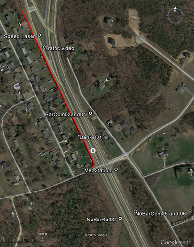
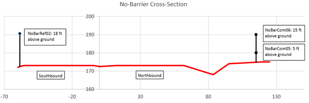
It is important to describe the source of the noise, which in most cases is traffic, but could also be other transportation and non-transportation sources, construction equipment, individual vehicle pass-bys, or an artificial noise. The example below describes traffic conditions (volume and speed) that occurred during a set of measurements:
“The source was constant free-flowing traffic traveling on Route XY. The team collected traffic volume and mix using a hand-held traffic counter [or, were recorded using a video camera] to obtain vehicle counts. Vehicles were counted and classified in the FHWA TNM five categories: automobiles (A); medium trucks (MT); heavy trucks (HT), Buses (B); and motorcycles (M). Vehicles were further grouped by direction [northbound/eastbound and southbound/westbound]. Averaged speeds were recorded for each direction. Table 18-1 shows vehicle counts and average speed for each test run.”
Include start and end times, especially if short-term measurements are being adjusted for worst-hour conditions based on a longer-term measurement at another site or if the measurement’s run was cut short due to unacceptable conditions (e.g., rain). Secondary sources that may have influenced the measurements such as other transportation modes, commercial, or industrial sources, should be documented.
The following example provides detailed instrument descriptions and an example of instrumentation log:
“The team measured sound levels using three ABC Model 888 class 1 precision integrating sound level meters, positioning the microphone/preamplifier combinations 1 ft (0.3 m) from the masts to minimize errors due to reflections from the mast structure. XYZ Model 0123 windscreens were placed atop each microphone to reduce the effects of wind-generated noise on the microphone diaphragm. Each Model 888 meter preprocessed and stored the measured sound level data. Each unit was programmed to continually measure and store A-weighted sound levels with “fast” exponential response characteristics at a rate of one data record per second, with energy-averaged one-minute equivalent sound levels also computed and stored. A passive microphone simulator established the electronic noise floor of each system prior to the measurement. In addition, the frequency response of each system was tested using pink noise generated by an ABC Model 20B random noise generator. Traffic speed was obtained with a DEF Doppler radar gun set up 25 ft (7.5 m) off the edge of the near travel lane, approximately 330 ft (100 m) west of the microphone centerline. The radar gun was directed at the departing westbound traffic, thus minimizing the possibility of individual vehicles slowing down after detecting the radar signal. A team member visually observed the radar’s digital display, and recorded continuously during each measurement period at a rate of approximately one reading every 10 seconds. A XYZ Model 405 video camera was set up on a nearby overpass to record pass-by traffic at the measurement site. The camera was time-synchronized with the Model 888 meters so that the noise data could be correlated with the traffic data. A Model 2000 pocket weather meter measured wind speed and temperature at a relatively exposed position and at an elevation approximately equal to that of the highest receiver position.”
Table 18-2 provides a sample of instrumentation log that includes instrumentation type (i.e., sound level meter, calibrator, radar gun, and video camera). The manufacturers’ recommended calibration cycle and the most recent calibration date should be recorded.
The following provides an example of how to describe meteorological conditions that occurred during noise measurements:
“A weather station continually recorded temperature, humidity, wind speed, and wind direction data. Wind speed and direction were measured at a height of 25 ft (7.5 m) above the ground (height equivalent to the highest microphone position); temperature and humidity were measured at a height of 5 ft (1.5 m) above the ground. In addition, a team member documented cloud cover periodically along with significant changes in weather conditions. After the measurements, the average wind speed and average wind direction relative to magnetic north (degrees) were computed for each five-minute test run. The five-minute average wind speed and direction were then used in the calculation of the vector component of wind speed in the x-y plane from the source to receiver for each test run.”
Table 18-3 presents meteorological data. Include start and end times to allow correlation with the sound level measurement data and traffic data.
The following text is an example of how to document roadway surface and adjacent ground surfaces.
“The roadway surface was composed of dense-graded asphalt concrete. The roadside terrain between the road and the receivers was relatively flat and composed of packed clay with low-cut grass. Table 18-4 includes a user key of FHWA TNM ground types to assist in assigning field conditions with modeling parameters.”
It is recommended that examples of pavement photographs and topography be added.
| Run # | Pavement 1 | Pavement 2 | Shoulder | Ground 1 | Ground 2 |
|---|---|---|---|---|---|
| 1 | Dense Grade | Dense Grade | P | FG | FG |
| 2 | Open Grade | Open Grade | P | W | W |
| 3 | Average | Average | P | PS | PS |
Below is an example of a written description of field measurement procedures:
“At the beginning of the measurement day, the team conducted a complete system check on the entire measurement system. To establish the electronic noise floor of each system, a passive microphone simulator was substituted for each microphone. A 30-second recording sample of pink noise tested the frequency response of each system. In addition, 30 seconds of calibration data were recorded at the beginning and end of the measurement day. Data were collected at a rate of one sample per second, with the computing and storing of one-minute equivalent sound levels. At the end of the measurement day, the sound level data stored in each Model 888, and the meteorological data and traffic volume video counts, were downloaded to a notebook computer and uploaded as a backup on the cloud for off-line processing.”
The following is an example of a description of the post-measurement data analysis with a table that shows the collected data (adjusted for calibration drift, if necessary):
“Processing of the noise data files stored on the notebook computer was accomplished off-line, using the utility support software in tandem with the field notes. The utility software produced a graphical history plot (noise level versus time) for examination of potentially contaminated data. These field notes were examined and all questionable data highlighted in the notes were removed. Table 18-5 includes the measurements.”
Include start and end times to allow correlation with the meteorological and traffic data, and for any adjustments that might need to be made if the measurement was cut short due to unacceptable conditions (e.g., rain). Also, include the measurement period duration and the measured sound level data (Leq) for each measurement run. Use an appendix to the measurement documentation if printouts or tables of the one-minute Leq data used to compute the runs’ results are needed.
The minimum separation-distance criteria were based on Caltrans’ California vehicle noise emission levels study.[118]
The Caltrans study included the following assumptions:
In general, when a vehicle approaches a measurement microphone at a constant speed, the observed sound level at the microphone relates to the vehicle position using the following equation:
Equation 19-1: Relationship of Sound Level to Vehicle Position
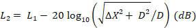
where:
L1 is the emission level of the subject vehicle, Vehicle 1, due entirely to Vehicle 1 at X1;
ΔX is the distance between X1 and X2, or the minimum separation distance to be determined, in the same units as D; and
D is the distance from the microphone to X1, or 50 ft (15 m) in this case.
L2 represents the emission level of Vehicle 1 transposed by some distance, ΔX, down the road. If it is assumed that Vehicle 1 and Vehicle 2 are the same, then L2 also represents the emission level of Vehicle 2, some distance ΔX from Vehicle 1.
Figure 19-1 shows a diagram of the relative position of vehicles X1 and X2 and the microphone.
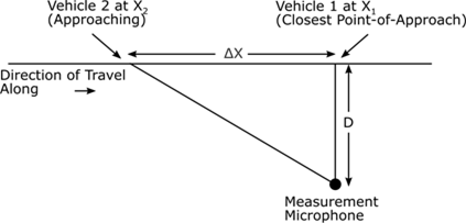
If other vehicles are in proximity of the subject vehicle to be measured, the measured sound level at the microphone for the subject vehicle may increase due to contamination. A maximum of 0.5 dB contamination is allowable.
Based on the 0.5-dB criterion, the next step is to determine the associated separation-distance criteria. Potential sources of contamination include contamination due to ambient noise and contamination due to other vehicles in proximity of the subject vehicle (Figure 19-2).
The maximum contamination due to ambient noise was determined to be 0.4 dB, assuming the ambient level is 10 dB less than the LAFmx of observed vehicles. Consequently, the maximum allowable contamination due to subsequent vehicles is 0.1 dB, based on the 0.5-dB contamination criterion.
The emission level due to a subsequent vehicle, Vehicle 2 in the case of Figure 19-1, must be at least 15.9 dB below that of the subject vehicle, Vehicle 1. This ensures that subsequent vehicles cause no more than 0.1-dB contamination. The next step is to determine the separation distance associated with the 15.9-dB requirement.
Substitute the following values into Equation 19-1 to solve for ΔX, the separation distance (Equation 19-2; also accounts for difference in sound level between vehicle 1 and vehicle 2):
L1 = LAFmx
L2 = LAFmx-15.9
D = 50 ft (15 m)
Equation 19-2: Required Distance to Avoid Contamination

where:
ΔX is the minimum separation distance to avoid contamination; and
Δ sound level = difference in sound level between vehicle 1 and vehicle 2.
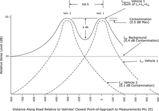
The minimum separation distance between similar vehicles required to ensure that the total contamination is not greater than 0.5 dB is 308 ft (93.9 m) for REMELs measured at 50 ft (15 m). Assuming a heavy truck is 10 dB louder than an automobile at comparable speeds, then the minimum separation distance between an automobile and a heavy truck is 985 ft (300.2 m).
In some cases, it is necessary to predict rail noise to help with establishing existing noise, to help with designing highway noise abatement, or to screen for rail noise impacts. This section provides a method for predicting rail noise for such cases.
There are two main steps in predicting rail noise levels following the General Assessment Method in FTA’s guidance:[119]
A simplification of this method is provided here to estimate rail noise sound levels. Shown below are details for each step based on FTA guidance combined with FRA guidance.[120] (If updated FTA and FRA guidance becomes available, reference such guidance for prediction method refinements.)
The most typical rail noise sources include freight rail, commuter rail, and light rail. Table 20-1 shows associated source levels (SEL) at a distance of 50 ft (15 m) and speed of 50 mph (80 kmh). Horns for freight rail and commuter rail are included in the table and should be applied for track segments within 0.25 mile (0.40 km) of a grade crossing. Special trackwork, crossing bells, and other stationary noise sources may also contribute to the sound at a receptor location. If such elements are suspected to contribute to the received noise levels, then reference FTA and FRA guidance to apply methods to further refine the predicted rail noise levels, including stationary sources. Compared to horns, elements such as crossing bells may be negligible. (There are some adjustments for track type and track crossovers included in the calculations in this section, in Table 20-2.)
*Note: Levels for other rail sources can be found in FTA guidance.
Incorporate other track, train, and operational parameters to predict noise at receiver locations, as appropriate:
After acquiring the appropriate information, use the equations in Table 20-2 to calculate a one-hour A-weighted equivalent sound level (shown as Leq(h) in the table) for each source type, based on the SELref levels shown in Table 20-2. Then combine the noise sources to obtain the worst hour sound level (shown as Leq(h), Combo in the table). It may be necessary to compute the combined totals with and without warning horns, since some neighborhoods along the corridor may be exposed to horn noise whereas others may not. To apply the day-night average sound level (DNL) metric, first calculate Lday and Lnight, then combine as shown to get Ldn, also shown in the table. Some sources may be different distances from the receiver of interest. An example is a case with both freight and light-rail tracks.
*Include only sources that apply.
Since different modes of transportation utilize different noise descriptors or “metrics,” it is necessary to convert from one noise metric to another to combine them into a single sound level. The subsection below describes the conversion of worst highway noise hour to the day-night average sound level (DNL). Appendix A includes noise metric definitions.
Before discussing conversion of worst hour highway traffic noise to DNL, note that DNL for traffic noise can be obtained using other methods. For predictions, it is possible to calculate DNL using the FHWA TNM; rather than the DNL calculations in FHWA TNM that assume equal traffic volumes every hour, an alternative is to use FHWA TNM to predict noise for each time of day, and combine the levels as shown in Appendix A, definition for Day-Night Average Sound Level. For measurements, it is possible to measure a representative equivalent sound level for each time of day then combine these to get DNL (again, see equations in the definition for Day-Night Average Sound Level in the Terminology section, Appendix A).
The following text discusses converting the worst hour highway traffic noise to DNL. The methods discussed here are based on those seen the 1982 FHWA document, Advanced Prediction and Abatement of Highway Traffic Noise[121] and Caltrans protocol document.[122] The conversions are an approximation of DNL based on the following assumptions: 1) 24-hour traffic mixes remain constant and that traffic speeds do not change; 2) peak hour traffic coincides with the worst hour Leq, which is often not true.
To convert worst hour Leq to DNL, make adjustments from a reference condition that assumes traffic volumes, speeds, and mixes remain constant throughout the entire 24 hours. In addition, know the following parameters:
Assuming that the worst hour equivalent sound level was already determined at the point of interest for the highway, the steps to determine DNL are as follows:
This approximation for the DNL incorporates the preceding assumptions. It also assumes that the volume percentages used in the charts in Table 21-1 and Table 21-2 are appropriate to both automobiles and heavy trucks. The method is relatively insensitive to these assumptions, however, since it has been found for many roadways studied that the DNL is equal to the peak hour Leq + 2 dB. This makes sense looking at the charts for typical traffic flows in which the peak hour percentage ranges from 8% to 12% and the nighttime percentage of the ADT ranges from 10% to 20%.
| Peak Hour % ADT | Δ1 (dB) |
|---|---|
| 4 | 0.2 |
| 5 | -0.8 |
| 6 | -1.6 |
| 7 | -2.3 |
| 8 | -2.8 |
| 9 | -3.3 |
| 10 | -3.8 |
| 11 | -4.2 |
| 12 | -4.6 |
| 13 | -4.9 |
| 14 | -5.3 |
| 15 | -5.6 |
| 17 | -6.1 |
| 20 | -6.8 |
| Day % ADT | Night % ADT | Δ2 (dB) |
|---|---|---|
| 100 | 0 | 0 |
| 95 | 5 | 1.6 |
| 90 | 10 | 2.8 |
| 85 | 15 | 3.7 |
| 80 | 20 | 4.5 |
| 75 | 25 | 5.1 |
| 70 | 30 | 5.7 |
| 65 | 35 | 6.2 |
| 60 | 40 | 6.6 |
The DNL for highway noise is expressed as
Equation 21-1: Convert Highway Worst Hour Leq to DNL (Ldn)
Ldn, highway = Leq(h), highway + Δ1 + Δ2 (dB)
An alternative to using the tables above is to apply the following equation, which corrects for the peak hour and nighttime penalty:
Equation 21-2: Convert Highway Worst Hour Leq to DNL (Ldn) without Tables
Ldn, highway = Leq(h), highway + 10 log10 (4.17 / P) + 10 log10 (D + 10N) (dB)
where:
Ldn, highway is the DNL for highway noise;
Leq(h), highway is the worst hour sound level for highway noise;
P is the peak hour volume % of ADT;
D is the daytime fraction of ADT (%volume/100);
N is the nighttime fraction of ADT (%volume/100); and
D + N = 1.
23 CFR Part 772. 2010. “Title 23: Highways - Part 772-Procedures for Abatement of Highway Traffic Noise and Construction Noise.” Federal Register, Volume 75, Number 133, pp. 39820–39839.
24 CFR Part 51 Subpart B. 1979 (amended 1996). “Noise Abatement and Control.” Federal Register, Volume 61 Number 59 pp. 13333 to 13335
AASHTO T 360-16. 2016. “Standard Method of Test for Measurement of Tire/Pavement Noise Using the On-Board Sound Intensity (OBSI) Method.” American Association of State Highway Transportation Officials, Washington, DC.
AASHTO TP 98-13 (2015). 2013 (update planned for 2017). “Standard Method of Test for Determining the Influence of Road Surfaces on Vehicle Noise Using the Statistical Isolated Pass-By (SIP) Method.” American Association of State Highway Transportation Officials, Washington, DC.
AASHTO TP 99. 2015 (update planned for 2017). “Standard Method of Test for Determining the Influence of Road Surfaces on Traffic Noise Using the Continuous-Flow Traffic Time-Integrated Method (CTIM).” American Association of State Highway Transportation Officials, Washington, DC.
Anderson, G.S., Lee, C.S., Fleming, G.G., and C.W. Menge. 1998. “FHWA Traffic Noise Model (FHWA TNM®), Version 1.0: User’s Guide.” John A. Volpe National Transportation Systems Center, Cambridge, MA.
Andrews, J., Buehler, D., Gill, H., and W.L. Bender. 2013. “Transportation and Construction Vibration Guidance Manual.” California Department of Transportation, Sacramento, CA.
ANSI/ASA S1.10-1986 (R2001). “Method for Calibration of Microphones.” Acoustical Society of America, Melville, New York, 2001.
ANSI/ASA S1.11-2014. “Octave-band and fractional-octave-band Filters—Part 1: Specifications.” Acoustical Society of America, Melville, New York.
ANSI/ASA S1.1-2013. “Acoustical Terminology.” Acoustical Society of America, Melville, New York.
ANSI/ASA S1.13-2005 (R2010). “Measurement of Sound Pressure Levels in Air.” Acoustical Society of America, Melville, New York.
ANSI/ASA S1.18-2010. “Determining the Acoustic Impedance of Ground Surfaces.” Acoustical Society of America, Melville, New York.
ANSI/ASA S1.25-1991 (R2017). “Specification for Personal Noise Dosimeters.” American National Standard, Melville, New York.
ANSI/ASA S1.26-1995 (R2014). “Method for Calculation of the Absorption of Sound by the Atmosphere.” Acoustical Society of America, Melville, New York.
ANSI/ASA S1.4 PART 1 2014. “American National Standard Electroacoustics – Sound Level Meters – Part 1: Specifications.” Acoustical Society of America, Melville, New York.
ANSI/ASA S1.4 PART 2 2014. “American National Standard Electroacoustics – Sound Level Meters – Part 2: Pattern Evaluation Test.” Acoustical Society of America, Melville, New York.
ANSI/ASA S1.4 PART 3 2014. “American National Standard Electroacoustics - Sound Level Meters - Part 3: Periodic Tests.” Acoustical Society of America, Melville, New York.
ANSI/ASA S12.8-1998 (R2013). “Methods for Determination of Insertion Loss of Outdoor Noise Barriers.,” Acoustical Society of America, Melville, New York.
ANSI/ASA S12.9-2013/Part 3. “Quantities and Procedures for Description and Measurement of Environmental Sound—Part 3: Short-term Measurements with an Observer Present.” Acoustical Society of America, Melville, New York.
ANSI/ASA Standard S12.18-1994 (R2009). “Procedures for Outdoor Measurement of Sound Pressure Level.” Acoustical Society of America, Melville, New York.
ASTM C384-04. 2016. “Standard Test Method for Impedance and Absorption of Acoustical Materials by Impedance Tube Method.” ASTM International, West Conshohocken, PA.
ASTM E1050-12. 2012. “Standard Test Method for Impedance and Absorption of Acoustical Materials Using a Tube, Two Microphones, and a Digital Frequency Analysis System.” ASTM International, West Conshohocken, PA.
ASTM E966-10e1. 2010. “Standard Guide for Field Measurements of Airborne Sound Insulation of Building Facades and Facade Elements.” ASTM International, West Conshohocken, PA.
Bajdek, C., Menge, C., Mazur, R.A., Pate, P., and J. Schroeder. 2015. “Recommended Best Practices for the Use of the FHWA Traffic Noise Model (TNM).” Federal Highway Administration, Washington, DC.
Beranek, L.L., and I.L. Vér. 1992. Noise and Vibration Control Engineering: Principles and Applications. John Wiley & Sons, Inc., New York, NY.
Bowlby, W., Williamson, R., Reiter, D., Patton, C., Pratt, G., Kaliski, K., Washburn, K., Rochat, J., El-Aassar, A., Knauer, H., Sanchez, G., and D. Barrett. 2015. “Field Evaluation of Reflected Noise from a Single Noise Barrier—Phase 1.” Web-only document 218, NCHRP 25-44. Transportation Research Board, Washington, DC.
Bradley, J. S., and Chu, W. T. 2002. “Errors when using façade measurements of incident aircraft noise.” 2002 International Congress and Exposition on Noise Control Engineering, Dearborn, MI.
Broch, J.T. 1975. Acoustic Noise Measurements. Brüel & Kjær, Denmark.
Brüel & Kjær. Condenser Microphones and Microphone Preamplifiers for Acoustic Measurements: Data Handbook. 1982. Brüel & Kjær, Denmark.
Donavan, P.R. 2006. “Comparative Measurements of Tire/Pavement Noise in Europe and the United States – NITE Study.” California Department of Transportation, Sacramento, CA.
Donavan, P.R., and D.M. Lodico. 2009. “Measuring Tire-Pavement Noise at the Source.” NCHRP 01-44. Transportation Research Board, Washington, DC.
Donavan, P.R., and D.M. Lodico. 2011. “Measuring Tire-Pavement Noise at the Source: Precision and Bias Statement.” NCHRP 01-44(1). Transportation Research Board, Washington, DC.
Fleming, G.G., and E.J. Rickley. 1991. “Parallel barrier effectiveness, Dulles noise barrier project.” The Journal of the Acoustical Society of America, Vol. 90, No. 4.
Fleming, G.G., and E.J. Rickley. 1994. “Performance evaluation of experimental highway noise barriers.” Final report. John A. Volpe National Transportation Systems Center, Cambridge, MA.
Fleming, G.G., and E.J., Rickley. 1993. “Development of National Reference Energy Mean Emission Levels for Constant-Flow Roadway Traffic: Test Plan.” John A. Volpe National Transportation Systems Center, Cambridge, MA.
Fleming, G.G., Rapoza, A.S., and C.S. Lee. 1995. “Development of the Reference Energy Mean Emission Level database for the FHWA Traffic Noise Model (FHWA TNM®), Version 1.0.” John A. Volpe National Transportation Systems Center, Cambridge, MA.
Hanson, C.E., Ross, J.C., and D.A. Towers. 2012. “High-Speed Ground Transportation Noise and Vibration Impact Assessment.” Federal Railroad Administration, Washington, DC.
Hanson, C.E., Towers, D.A., and L.D. Meister. 2006. “Transit Noise and Vibration Impact Assessment.” Federal Transit Administration, Washington, DC.
Harris Miller Miller & Hanson, Inc. 2006. “CREATE Railroad Noise Model User Guide.” Federal Railroad Administration, Washington, DC.
Harris Miller Miller & Hanson, Inc., Bowlby & Associates, Inc., Environmental Acoustics, Anderson, G.S., and D.E. Barrett. 2014. “Supplemental Guidance on the Application of FHWA’s Traffic Noise Model (TNM).” NCHRP 25-34. Transportation Research Board, Washington, DC.
Harris, C.M. (ed.). 1991. Handbook of Acoustical Measurements and Noise Control. McGraw-Hill, New York, NY.
Hastings, A.L., and J.L. Rochat. 2010. “Ground and Pavement Effects using FHWA’s Traffic Noise Model® 2.5.” John A. Volpe National Transportation Systems Center, Cambridge, MA.
Hendricks, R.W. 1987. “California Vehicle Noise Emission Levels.” California Department of Transportation, Sacramento, CA.
Hendricks, R.W. 1991. “Field Evaluation of Acoustical Performance of Parallel Highway Noise Barriers Along Route 99 in Sacramento, California.” California Department of Transportation, Sacramento, CA.
Hendriks, R.W., and J. Hecker. 1989. “Parallel Noise Barrier Report: A Noise Absorptive Demonstration Project.” California Department of Transportation, Sacramento, CA.
Hendriks, R.W., Rymer, B., Buehler, D., and J. Andrews. 2013. “Technical Noise Supplement to the Traffic Noise Analysis Protocol: A Guide for Measuring, Modeling, and Abating Highway Operation and Construction Noise Impacts.” California Department of Transportation, Sacramento, CA.
IEC 60942:2003. “Electroacoustics - Sound Calibrators.” International Electrotechnical Commission, Denmark.
IEC 61265:1995. “Electroacoustics - Instruments for measurement of aircraft noise - Performance requirements for systems to measure one-third octave-band sound pressure levels in noise certification of transport-category aeroplanes.” International Electrotechnical Commission, Denmark.
ISO 10534-1:1996 (confirmed in 2016). “Acoustics—Determination of sound absorption coefficient and impedance in impedance tubes—Part 1: Method using standing wave ratio.” International Organization for Standardization, Geneva, Switzerland.
ISO 10534-2:1998 (confirmed in 2015). “Acoustics—Determination of sound absorption coefficient and impedance in impedance tubes—Part 2: Transfer-function method.” International Organization for Standardization, Geneva, Switzerland.
ISO 10844:2014. “Acoustics—Specification of test tracks for measuring noise emitted by road vehicles and their tyres.” International Organization for Standardization, Geneva, Switzerland.
ISO 11819-1:1997 (confirmed in 2013). “Acoustics—Measurement of the influence of road surfaces on traffic noise—Part 1: Statistical Pass-By Method.” International Organization for Standardization, Geneva, Switzerland.
ISO 11819-2:2017. “Acoustics—Measurement of the influence of road surfaces on traffic noise—Part 2: The close-proximity method.” International Organization for Standardization, Geneva, Switzerland.
ISO 12354-1:2007. “Building acoustics -- Estimation of acoustic performance of buildings from the performance of elements -- Part 1: Airborne sound insulation between rooms.” International Organization for Standardization, Geneva, Switzerland.
ISO 13325:2003 (confirmed in 2008). “Tyres—Coast-by Methods for measurement of tyre-to-road sound emission.” International Organization for Standardization, Geneva, Switzerland.
ISO 13472-1:2002 (confirmed in 2012). “Acoustics—Measurement of sound absorption properties of road surfaces in situ—Part 1: Extended surface method.” International Organization for Standardization, Geneva, Switzerland.
ISO 13472-2:2010 (confirmed in 2013). “Acoustics—Measurement of sound absorption properties of road surfaces in situ—Part 2: Spot method for reflective surfaces.” International Organization for Standardization, Geneva, Switzerland.
ISO 362-1:2015. “Measurement of noise emitted by accelerating road vehicles.” International Organization for Standardization, Geneva, Switzerland.
ISO 5128:1980 (confirmed in 2013). “Acoustics—Measurement of noise inside motor vehicles.” International Organization for Standardization, Geneva, Switzerland.
ISO 9613-1:1993 (confirmed in 2015). “Acoustics—Attenuation of sound during propagation outdoors—Part 1: Calculation of the absorption of sound by the atmosphere.” International Organization for Standardization, Geneva, Switzerland.
ISO/PAS 11819-4:2013 (confirmed in 2017). “Acoustics—Method for measuring the influence of road surfaces on traffic noise—Part 4: SPB method using backing board.” International Organization for Standardization, Geneva, Switzerland.
ISO/TS 11819-3:2017. “Acoustics—Measurement of the influence of road surfaces on traffic noise—Part 3: Reference tyres.” International Organization for Standardization, Geneva, Switzerland.
Lau, M.C., Lee, C.S.Y., Rochat, J.L., Boeker, E.R., and G.G. Fleming. 2004. “FHWA Traffic Noise Model® User’s Guide (Version 2.5 Addendum).” John A. Volpe National Transportation Systems Center, Cambridge, MA.
LAX website LAX Internet Flight Tracking System—Noise Management website. http://www.lawa.org/welcome_lax.aspx?id=32 (As of August 22, 2017).
Lee, C.S.Y., and G.G. Fleming. 1996. “Measurement of Highway-Related Noise.” Federal Highway Administration, Washington, DC.
McGillem, C.D., and G.R. Cooper. 1984. Continuous and Discrete Signal and System Analysis. Holt Rinehart & Winston, New York, NY (3rd Edition 1991, Oxford University Press).
MPH Industries, “Operator’s Manual for Stationary Radar, Model K-15 II Hand Held Unit.” 1985. MPH Industries, Inc., Owensboro, KY.
Noise Assessment Guidelines.” 2009. US Department of Housing and Urban Development, Washington, DC.
Peterson, A.P.G. 1980. Handbook of Noise Measurement. General Radio Company, Concord, MA.
Plovsing, B. 2007. “Proposal for Nordtest Method: Nord2000 - Prediction of Outdoor Sound Propagation.” Danish Electronics Light & Acoustics, Hørsholm, Denmark.
Reherman, C.N., Rochat, J.L., Thalheimer, E.S., Lau, M.C., Fleming, G.G., Ferroni, M., and C. Corbisier. 2006. “FHWA Roadway Construction Noise Model, User’s Guide.” John A. Volpe National Transportation Systems Center, Cambridge, MA.
Rickley, E.J., Ingard, U., Cho, Y.C., and R.W. Quinn. 1978. “Roadside Barrier Effectiveness, Noise Measurement Program.” John A. Volpe National Transportation Systems Center, Cambridge, MA.
Rochat, J.L., and D.R. Read. 2013. “Effective flow resistivity of highway pavements.” The Journal of the Acoustical Society of America, Vol. 134, No. 6.
Rochat, J.L., Donavan, P., Seybert, A., and T. Dare. 2012. “Pavement sound absorption measurements in the U.S.” Proceedings of InterNoise2012, New York, NY.
Rochat, J.L., Hastings, A.L., Read, D.R., and M.C. Lau. 2012. “FHWA Traffic Noise Model (TNM) Pavement Effects Implementation Study: Progress Report 1.” John A. Volpe National Transportation Systems Center, Cambridge, MA.
SAE ARP 4221/1. 2012. “Monitoring Aircraft Noise and Operations in the Vicinity of Airports: System Description, Acquisition, and Operation.” SAE International.
SAE ARP 5534. 2013. “Application of Pure-Tone Atmospheric Absorption Losses to One-Third Octave-Band Data.” SAE International.
SAE J1477_200005. “Measurement of Interior Sound Levels of Light Vehicles.” SAE International.
SAE J2805_201511. “Measurement of Noise Emitted by Accelerating Road Vehicles.” SAE International.
SAE J2920. “Measurement of Tire/Pavement Noise Using Sound Intensity.” SAE International.
SAE J57_201405. “Sound Level of Highway Truck Tires (STABILIZED May 2014).” SAE International.
SoundPLAN GmbH, “SoundPLAN® User’s Manual.” 2012. Braunstein + Berndt GmbH.
U.S. Department of Housing and Urban Development, “The Noise Guidebook.” 2009, Washington, DC.
U.S. Department of Housing and Urban Development. Website DNL Calculator https://www.hudexchange.info/environmental-review/dnl-calculator/ (As of August 22, 2017).
U.S. Department of Transportation, “Advanced Prediction and Abatement of Highway Traffic Noise.” 1982 (recreated November 2016). Federal Highway Administration, Washington, DC.
U.S. Department of Transportation, “Tire-Pavement Noise: Strategic Planning Workshop.” 2004. Federal Highway Administration, Washington, DC.
U.S. Department of Transportation, “Highway Traffic Noise: Analysis and Abatement Guidance.” 2011. Federal Highway Administration, Washington, DC.
U.S. Department of Transportation, webpage: Air Traffic Activity System (ATADS) > Airport Operations, https://aspm.faa.gov/opsnet/sys/Airport.asp (As of August 21, 2017).
U.S. Department of Transportation. Noise Measurement Field Guide, Report No. FHWA-HEP-18-066, Federal Highway Administration, Washington, D.C., 2017.
Yerges, L.F. 1978. Sound, Noise, and Vibration Control. Krieger Publishing Company, New York, NY.
Zubrow, A., Hwang, S., Ahearn, M., Hansen, A., Koopmann, J., and G. Solman. 2016. “Aviation Environmental Design Tool (AEDT) 2c User Guide.” John A. Volpe National Transportation Systems Center, Cambridge, MA.
[1] “Procedures for Abatement of Highway Traffic Noise and Construction Noise,” Code of Federal Regulations, Title 23, Part 772 (23 CFR 772), Federal Register, Volume 75, Number 133, pages 39820-39839, July 13, 2010.
[2] Measurement of Highway-Related Noise, Report No. FHWA-PD-96-5, Federal Highway Administration, Washington, DC, 1996.
[3] The Federal Highway Administration noise regulation in 23 CFR 772 requires a state highway agency to study traffic noise impacts for proposed Federal or Federal-aid highway projects defined as Type I, which includes several categories involving construction at a new location or reconstruction of an existing highway that increases the number of through-traffic lanes or significantly changes the horizontal or vertical alignment.
[4] Screening distances for vibration found in Hanson, et al., Transit Noise and Vibration Impact Assessment, Report No. FTA-VA-90-1003-06, Federal Transit Administration, Washington, DC, 2006.
[5] The FHWA noise regulation in 23 CFR 772 defines a Type II project as a Federal or Federal-aid highway project for noise abatement on an existing highway. It is assumed that no action is being taken on the highway that would be categorized as a Type I project. The regulation provides a framework for the noise study for a Type II project.
[6] 24 CFR Part 51 Subpart B - Noise Abatement and Control, US Department of Housing and Urban Development, 1979, amended 1996.
[7] See “The Noise Guidebook,” US Department of Housing and Urban Development (updated 2009), or consult with a HUD official.
[8] Bajdek, C., Menge, C., Mazur, R.A., Pate, P., and Schroeder, J., Recommended Best Practices for the Use of the FHWA Traffic Noise Model (TNM), FHWA-HEP-16-018, FHWA, Washington, DC, 2015.
[9] Noise Measurement Field Guide, Federal Highway Administration, Washington, D.C., 2017.
[10] There is a typographical error in the text in 23 CFR 772 in Sec. 772.11(a). Subsections (1) and (2) state: “(1) For projects on new alignments, determine traffic noise impacts by field measurements. (2) For projects on existing alignments, predict existing and design year traffic noise impacts.” In both cases, the word “impacts” should be “levels.”
[11] Section 772.11(d) (3) of 23 CFR 772 calls for the use of an integrating sound level meter or analyzer, which automatically measures Leq.
[12] The electrical noise floor of the sound level measurement system (meter/analyzer, microphone/preamplifier, and microphone extension cable, if used) can affect the accuracy of a sound level measurement. Sound pressure levels that are at least 10 dB higher than the floor should be relatively unaffected. Levels within 5 dB of the noise floor are not valid. Establishing the noise floor is important for research measurements or measurements in a low-noise environment or done with a long cable run. The instrument manufacturer should be able to state the electrical noise floor (preferably, as a function of frequency). It can also be measured in the field using a microphone simulator (often called a “dummy mic”) during the calibration procedure. More information on a microphone simulator is in Appendix B.
[13] Temperature and humidity have small effects on measured traffic noise levels at the typical distances of concern, to a much lesser degree than temperature lapse rate and wind shear/direction.
[14] Measurement of Highway-Related Noise (Report No. FHWA-PD-96-5), FHWA, Washington, DC, 1996; “Methods for Determination of Insertion Loss of Outdoor Noise Barriers,” American National Standard, ANSI/ASA S12.8-1998 (R2013), Acoustical Society of America, Melville, New York, 2013.
[15] “Measurement of Sound Pressure Levels in Air,” ANSI/ASA S1.13-2005 (R2010), Acoustical Society of America, Melville, New York, 2010.
[16] ANSI/ASA S1.13-2005 (R2010) states “The total ambient sound that exists at a given point in space is usually due to a composite of many different sounds with different strengths and frequency content. The composite sound may be a combination of background noise and sound from a single identifiable source.” In this handbook, background is defined as ambient sound excluding the source of interest.”
[17] There is a typographical error in the text in 23 CFR 772 in Sec. 772.11(a). Subsections (1) and (2) state: “(1) For projects on new alignments, determine traffic noise impacts by field measurements. (2) For projects on existing alignments, predict existing and design year traffic noise impacts.” In both cases, the word “impacts” should be “levels.”
[18] Highway Traffic Noise: Analysis and Abatement Guidance, Federal Highway Administration, Washington, DC, December 2011, pp. 31–32.
[19] Highway Traffic Noise: Analysis and Abatement Guidance, Federal Highway Administration, Washington, DC, December 2011, p. 31.
[20] Menge, C., W. Bowlby, G. Anderson, H. Knauer, A. El-Aassar, D. Barrett, et al, Supplemental Guidance on the Application of FHWA’s Traffic Noise Model (TNM), NCHRP Report 791, NAS, TRB, Washington, DC, 2014.
[21] Based on figure 5 of: Donavan, P.R., Comparative Measurements of Tire/Pavement Noise in Europe and the United States – NITE Study, Report No. FHWA/CA/MI-2006/09, California Department of Transportation, Sacramento, CA, 2006.
[22] FHWA TNM version 2.5 does not have the capability of modeling reflections off single vertical walls, such as the front or back of a house. Placing a validation site near a vertical reflecting surface could increase the sound level and invalidate the validation effort. FHWA TNM version 3.0 will have that capability if the user designates that wall as a reflecting surface for user-designated roadway segments.
[23] “Quantities and Procedures for Description and Measurement of Environmental Sound—Part 3: Short-term Measurements with an Observer Present,” ANSI/ASA S12.9-2013/Part 3, Acoustical Society of America, Melville, New York, 2013.
[24] Sections 9.6.2 and 9.6.3 of ASTM E966-10e1, referencing: Bradley, J. S. and Chu, W. T., “Errors When using Façade Measurements of Incident Aircraft Noise,” 2002 International Congress and Exposition on Noise Control Engineering, Dearborn, MI, August 19-21, 2002.
[25] Section 772.11(d) (3) of 23 CFR 772 requires the use of an integrating sound level meter or analyzer, which automatically measures Leq.
[26] The electrical noise floor of the sound level measurement system (meter/analyzer, microphone/preamplifier and microphone extension cable, if used) can affect the accuracy of a sound level measurement. Sound pressure levels that are at least 10 dB higher than the floor should be relatively unaffected. Levels within 5 dB of the noise floor are not valid. Establishing the noise floor is important for research measurements or measurements in a low-noise environment or done with a long cable run. The instrument manufacturer should be able to state the electrical noise floor (preferably, as a function of frequency). It can also be measured in the field using a microphone simulator (often called a “dummy mic”) during the calibration procedure. More information on a microphone simulator is in Appendix B.
[27] Menge, C., W. Bowlby, G. Anderson, H. Knauer, A. El-Aassar, D. Barrett, et al, Supplemental Guidance on the Application of FHWA’s Traffic Noise Model (TNM), NCHRP Report 791, NAS, TRB, Washington, DC, 2014.
[28] SoundPLAN® User’s Manual, Braunstein + Berndt GmbH, January 2012 (including update information for Version 7.2 – November 2012).
[29] Delta, “Proposal for Nordtest Method: Nord2000 – Prediction of Outdoor Sound Propagation,” January 2010.
[30] NCHRP Report 791 and its appendices are available online. Appendix J of that report give more details on the meteorological research.
[31] Advanced Prediction and Abatement of Highway Traffic Noise, Federal Highway Administration, Office of Environmental Policy, June 1982.
[32] Hanson, et al., Transit Noise and Vibration Impact Assessment, Report No. FTA-VA-90-1003-06, Federal Transit Administration, Washington, DC, 2006.
[33] Hanson, et al., Transit Noise and Vibration Impact Assessment, Report No. FTA-VA-90-1003-06, Federal Transit Administration, Washington, DC, 2006.
[34] Harris Miller Miller & Hanson, CREATE Railroad Noise Model User Guide, prepared for Federal Railroad Administration, 2006.
[35] HUD Exchange DNL Calculator, US Department of Housing and Urban Development.
[36] Noise Assessment Guidelines, US Department of Housing and Urban Development, Office of Policy Development and Research, 2009.
[37] LAX Internet Flight Tracking System—Noise Management website, Los Angeles International Airport.
[38] “Aircraft Noise and Operations in the Vicinity of Airports: System Description, Acquisition, and Operation,” SAE ARP 4221/1, 2012.
[39] Zubrow, et al., AEDT Version 2c User Guide, Report No. DOT-VNTSC-FAA-16-16, US Department of Transportation, Volpe National Transportation Systems Center, Cambridge, MA, 2016.
[40] Air Traffic Activity System (ATADS) > Airport Operations website, Federal Aviation Administration.
[41] “Standard Guide for Field Measurements of Airborne Sound Insulation of Building Facades and Facade Elements,” ASTM E966-10e1, ASTM International, West Conshohocken, PA, 2010.
[42] Highway Traffic Noise: Analysis and Abatement Guidance, Federal Highway Administration, Washington, DC, December 2011, p. 30.
[43] For example, roughly 662 ft2 (61.5 m2) for an 8-ft (2.4-m) high ceiling.
[44] For example, if the wall is 40 ft (12 m) long by 10 ft (3 m) high, then there would be four microphone positions.
[45] ASTM E966 uses this close-in microphone location. Take care about not overloading the sound level instrument circuitry because the signal should be loud enough to be 5–10 dB above background inside a building with an OINR as much as 35 dB. If overloading occurs, then the reference microphone should be moved back to a distance where no overload occurs, assuming that this more distant reference location can be replicated at the building site.
[46] ASTM E966-10e1 also states that measurements could be made at angles of 15, 30, 45, 60, and 75° and averaged on a weighted basis. Refer to sections 8.2.3 and 8.6.1 of the ASTM document for details.
[47] The electrical noise floor of the sound level measurement system (meter/analyzer, microphone/preamplifier, and microphone extension cable, if used) can affect the accuracy of a sound level measurement. Sound pressure levels that are at least 10 dB higher than the floor should be relatively unaffected. Levels within 5 dB of the noise floor are not valid. Establishing the noise floor is important for research measurements or measurements in a low-noise environment or done with a long cable run. The instrument manufacturer should be able to state the electrical noise floor (preferably, as a function of frequency). It can also be measured in the field using a microphone simulator (often called a “dummy mic”) during the calibration procedure. More information on a microphone simulator is in Appendix B.
[48] Hanson, et al., Transit Noise and Vibration Impact Assessment, Report No. FTA-VA-90-1003-06, Federal Transit Administration, Washington, DC, 2006.
[49] Hanson, et al., Transit Noise and Vibration Impact Assessment, Report No. FTA-VA-90-1003-06, Federal Transit Administration, Washington, DC, 2006.
[50] FTA is expected to adopt the FRA Krad value of -5 dB.
[51] Hanson, et al., Transit Noise and Vibration Impact Assessment, Report No. FTA-VA-90-1003-06, Federal Transit Administration, Washington, DC, 2006.
[52] Hanson, et al., High-Speed Ground Transportation Noise and Vibration Impact Assessment, Report No. DOT/FRA/OFD-12/15, Federal Railroad Administration, Washington, DC, 2012.
[53] “Exterior Sound Level Measurement Procedure for Powered Mobile Construction Equipment.” Society of Automotive Engineers’ Standard, SAE J88a Society of Automotive Engineers, 1976.
[54] “Sound Levels for Engine Powered Equipment.” Society of Automotive Engineers’ Standard, SAE J952b, Society of Automotive Engineers, 1976.
[55] The electrical noise floor of the sound level measurement system (meter/analyzer, microphone/preamplifier, and microphone extension cable, if used) can affect the accuracy of a sound level measurement. Sound pressure levels that are at least 10 dB higher than the floor should be relatively unaffected. Levels within 5 dB of the noise floor are not valid. Establishing the noise floor is important for research measurements or measurements in a low-noise environment or done with a long cable run. The instrument manufacturer should be able to state the electrical noise floor (preferably, as a function of frequency). It can also be measured in the field using a microphone simulator (often called a “dummy mic”) during the calibration procedure. More information on a microphone simulator is in Appendix B.
[56] Andrews, et al., Transportation and Construction Vibration Guidance Manual, California DOT, Sacramento, CA, 2013.
[57] Hanson, et al., Transit Noise and Vibration Impact Assessment, Report No. FTA-VA-90-1003-06, Federal Transit Administration, Washington, DC, 2006.
[58] “Methods for Determination of Insertion Loss of Outdoor Noise Barriers,” ANSI/ASA S12.8-1998 (R2013). Acoustical Society of America, Melville, New York, 2013.
[59] “Determining the Acoustic Impedance of Ground Surfaces,” ANSI/ASA S1.18-2010, Acoustical Society of America, Melville, New York, 2010.
[60] Hastings, A.L. and J.L. Rochat, Ground and Pavement Effects using FHWA’s Traffic Noise Model 2.5, Report DOT-VNTSC-FHWA-10-01 and FHWA-HEP-10-021, John A. Volpe National Transportation Systems Center, Acoustic Facility, Cambridge MA, April 2010.
[61] Menge, C., W. Bowlby, G. Anderson, H. Knauer, A. El-Aassar, D. Barrett, et al, Supplemental Guidance on the Application of FHWA’s Traffic Noise Model (TNM), NCHRP Report 791, NAS, TRB, Washington, DC, 2014.
[62] “Methods for Determination of Insertion Loss of Outdoor Noise Barriers,” ANSI/ASA S12.8-1998 (R2013). Acoustical Society of America, Melville, New York, 2013; Fleming, G.G. and E.J. Rickley, Performance Evaluation of Experimental Highway Noise Barriers, Report No. FHWA- RD-94-093. Cambridge, MA: John A. Volpe National Transportation Systems Center, April 1994.
[63] Fleming, G.G. and E.J. Rickley, Performance Evaluation of Experimental Highway Noise Barriers, Report No. FHWA- RD-94-093. Cambridge, MA: John A. Volpe National Transportation Systems Center, April 1994.
[64] Temperature and humidity generally have small effects on measured traffic noise levels at the typical distances of concern, to a much lesser degree than temperature lapse rate and wind shear/direction.
[65] Menge, C., W. Bowlby, G. Anderson, H. Knauer, A. El-Aassar, D. Barrett, et al, Supplemental Guidance on the Application of FHWA’s Traffic Noise Model (TNM), NCHRP Report 791, NAS, TRB, Washington, DC, 2014.
[66] Johnson, D.L., Marsh, A.H., and Harris, C.M. Acoustical Measurement Instruments, Handbook of Acoustical Measurements and Noise Control, New York, Columbia University, 1991; Hendriks, R.W. and J. Hecker, Parallel Noise Barrier Report: A Noise Absorptive Demonstration Project, Sacramento, CA, California Department of Transportation, July 1989.
[67] The electrical noise floor of the sound level measurement system (meter/analyzer, microphone/preamplifier, and microphone extension cable, if used) can affect the accuracy of a sound level measurement. Sound pressure levels that are at least 10 dB higher than the floor should be relatively unaffected. Levels within 5 dB of the noise floor are not valid. Establishing the noise floor is important for research measurements or measurements in a low-noise environment or done with a long cable run. The instrument manufacturer should be able to state the electrical noise floor (preferably, as a function of frequency). It can also be measured in the field using a microphone simulator (often called a “dummy mic”) during the calibration procedure. More information on a microphone simulator is in Appendix B.
[68] Bowlby, W., R. Williamson, D. Reiter, C. Patton, G. Pratt, K. Kaliski, K. Washburn, J. Rochat, A. El-Aassar, H. Knauer, G. Sanchez, and D. Barrett, Field Evaluation of Reflected Noise from a Single Noise Barrier—Phase 1, Web-only Document 218, NCHRP, TRB, National Academies, 2015.
[69] Hendricks, R.W., Field Evaluation of Acoustical Performance of Parallel Highway Noise Barriers Along Route 99 in Sacramento, California, Report No. FHWA/CA/TL-91/01, Sacramento, CA, California Department of Transportation, Division of New Technology, Materials and Research, January 1991; Fleming, G.G. and E.J. Rickley, Parallel Barrier Effectiveness: Dulles Noise Barrier Project, Report No. FHWA-RD-90-105, Cambridge, MA, John A. Volpe National Transportation Systems Center, May 1990.
[70] Anderson, G.S., Lee, C.S., Fleming, G.G., and Menge, C.W., FHWA Traffic Noise Model (FHWA TNM®), Version 1.0: User’s Guide, Report No. FHWA-PD-96-009, Cambridge, MA, John A. Volpe National Transportation Systems Center, January 1998; Lau, M.C., Lee, C.S.Y., Rochat, J.L., Boeker, E.R., and Fleming, G.G., FHWA Traffic Noise Model® User’s Guide (Version 2.5 Addendum), Cambridge, MA, John A. Volpe National Transportation Systems Center, April 2004.
[71] Fleming, G.G., Rapoza, A.S., and Lee C.S., Development of the Reference Energy Mean Emission Level database for the FHWA Traffic Noise Model (FHWA TNM®), Version 1.0, Report No. FHWA-PD-96-008, Cambridge, MA, John A. Volpe National Transportation Systems Center, November 1995; Fleming, G.G., Rickley, E.J., Development of National Reference Energy Mean Emission Levels for Constant-Flow Roadway Traffic: Test Plan, Letter Report No. DTS-75-HW327-LR2, Cambridge, MA, John A. Volpe National Transportation Systems Center, September 1993.
[72] Rochat, J.L., Hastings, A.L., Read, D.R. and Lau, M.C., FHWA Traffic Noise Model (TNM) Pavement Effects Implementation Study: Progress Report 1, Report No. DOT-VNTSC-FHWA-12-01, USDOT John A. Volpe National Transportation Systems Center, Cambridge, MA, January 2012.
[73] Fleming, G.G., Rapoza, A.S., and Lee C.S., Development of the Reference Energy Mean Emission Level Database for the FHWA Traffic Noise Model (FHWA TNM®), Version 1.0, Report No. FHWA-PD-96-008, Cambridge, MA, John A. Volpe National Transportation Systems Center, November 1995.
[74] The electrical noise floor of the sound level measurement system (meter/analyzer, microphone/preamplifier, and microphone extension cable, if used) can affect the accuracy of a sound level measurement. Sound pressure levels that are at least 10 dB higher than the floor should be relatively unaffected. Levels within 5 dB of the noise floor are not valid. Establishing the noise floor is important for research measurements or measurements in a low-noise environment or done with a long cable run. The instrument manufacturer should be able to state the electrical noise floor (preferably, as a function of frequency). It can also be measured in the field using a microphone simulator (often called a “dummy mic”) during the calibration procedure. More information on a microphone simulator is in Appendix B.
[75] Section 8.3 of “Standard Method of Test for Determining the Influence of Road Surfaces on Vehicle Noise Using the Statistical Isolated Pass-By (SIP),” TP 98-13, American Association of State Highway and Transportation Officials, Washington, DC, 2015, gives a minimum number of 30 samples and a desirable number of 100 without a speed range constraint. The values in the table are in recognition that on a given road the speed variation will be such that a number between minimum and desirable will be achieved.
[76] See in particular Appendix B, page 73, of Rochat, J.L., Hastings, A.L., Read, D.R. and Lau, M.C., FHWA Traffic Noise Model (TNM) Pavement Effects Implementation Study: Progress Report 1, Report No. DOT-VNTSC-FHWA-12-01, USDOT John A. Volpe National Transportation Systems Center, Cambridge, MA, January 2012.
[77] Anderson, G.S., Lee, C.S., Fleming, G.G., and Menge, C.W., FHWA Traffic Noise Model (FHWA TNM®), Version 1.0: User’s Guide, Report No. FHWA-PD-96-009, Cambridge, MA, John A. Volpe National Transportation Systems Center, January 1998; Fleming, G.G., Rapoza, A.S., and Lee C.S., Development of the Reference Energy Mean Emission Level Database for the FHWA Traffic Noise Model (FHWA TNM®), Version 1.0, Report No. FHWA-PD-96-008, Cambridge, MA, John A. Volpe National Transportation Systems Center, November 1995.
[78] Measuring Tire/Pavement Noise at the Source, National Cooperative Highway Research Program Report 630, 2009.
[79] Measuring Tire-Pavement Noise at the Source: Precision and Bias Statement, National Cooperative Highway Research Program Report for Project 1-44(1), 2011.
[80] Fleming, G., Rapoza, A., and Lee, C., Development of National Reference Energy Mean Emission Levels for the FHWA Traffic Noise Model (FHWA TNM), Version 1.0, Report No. DOT-VNTSC-FHWA-96-2, U.S. Department of Transportation, 1996.
[81] “FHWA TNM Pavement Effects Implementation Study: Progress Report 1”, Report No. DOT-VNTSC-FHWA-12-01, January 2012.
[82] Judith L. Rochat and David R. Read, “Effective flow resistivity of highway pavements,” J. Acoust. Soc. Am. 134(6), Pt. 2, December 2013.
[83] Judith L. Rochat, Paul Donavan, Andrew Seybert, and Tyler Dare, “Pavement sound absorption measurements in the U.S.,” Proceedings of Inter-Noise 2012.
[84] Judith L. Rochat, Paul Donavan, Andrew Seybert, and Tyler Dare, “Pavement sound absorption measurements in the U.S.,” Proceedings of Inter-Noise 2012.
[85] “Method for Determining the Acoustic Impedance of Ground Surfaces,” ANSI/ASA S1.18-2010, Acoustical Society of America, Melville, New York, 2010.
[86] “Electroacoustics – Sound level meters – Part 1: Specifications,” ANSI/ASA S1.4-2014/Part 1. Acoustical Society of America, Melville, New York, 2006.
[87] Peterson, A., Gross, E., Handbook of Noise Measurement, Concord, MA, General Radio Company, 1963.
[88] Rickley, E.J., Ingard, U., Cho, Y.C., and Quinn, R.W., Roadside Barrier Effectiveness: Noise Measurement Program, Report No. NHTSA-78-24, John A. Volpe National Transportation Systems Center, 1978.
[89] Condenser Microphones and Microphone Preamplifiers, Denmark, Brüel & Kjær Instruments, Inc., September 1982.
[90] Johnson, D.L., Marsh, A.H., and Harris, C.M. Acoustical Measurement Instruments. Handbook of Acoustical Measurements and Noise Control. New York: Columbia University, 1991.
[91] Peterson, A., Gross, E., Handbook of Noise Measurement, Concord, MA, General Radio Company, 1963.
[92] Broch, J.T. Acoustic Noise Measurements. Denmark: Brüel & Kjær Instruments, Inc., June 1975.
[93] “Electroacoustics, Instruments for measurement of aircraft noise - Performance requirements for systems to measure one-third octave-band sound pressure levels in noise certification of transport-category aeroplanes.” International Electrotechnical Commission Standard, IEC Draft Standard 1265, Denmark, International Electrotechnical Commission, 1999.
[94] “Method for Calibration of Microphones,” ANSI/ASA S1.10-1986 (R2001), Acoustical Society of America, Melville, New York, 2001.
[95] “Electroacoustics – Sound level meters – Part 1: Specifications,” ANSI/ASA S1.4-2014/Part 1, Acoustical Society of America, Melville, New York, 2006.
[96] “Specification for Octave-Band and Fractional-Octave-Band Analog and Digital Filters,” ANSI/ASA S1.11-2014, Acoustical Society of America, Melville, New York 2014.
[97] Hanson, et al., Transit Noise and Vibration Impact Assessment, Report No. FTA-VA-90-1003-06, Federal Transit Administration, Washington, DC, 2006.
[98] McGillem, C.D., Cooper, G.R., Continuous and Discrete Signal and System Analysis, New York, Purdue University, School of Electrical Engineering, 1984.
[99] “Electroacoustics - Instruments for measurement of aircraft noise - Performance requirements for systems to measure one-third-octave-band sound pressure levels in noise certification of transport-category aeroplanes,” International Electrotechnical Commission Standard, IEC Draft Standard 61265:1995, Denmark: International Electrotechnical Commission, 1995.
[100] Yerges, L.F. Sound, Noise and Vibration Control, New York, Van Nostrand Reinhold Company, 1978.
[101] “Electroacoustics - Sound Calibrators,” International Electrotechnical Commission Standard, IEC Standard 60942:2003, Denmark, International Electrotechnical Commission, 2003.
[102] “Measurement of Sound Pressure Levels in Air,” American National Standard, ANSI/ASA S1.13-2005 (R2010), Acoustical Society of America, Melville, New York, 2010.
[103] Hendricks, R.W., Field Evaluation of Acoustical Performance of Parallel Highway Noise Barriers along Route 99 in Sacramento, California, Report No. FHWA/CA/TL-91/01, Sacramento, CA, California Department of Transportation, Division of New Technology, Materials and Research, January 1991.
[104] “Procedures for Outdoor Measurement of Sound Pressure Level” American National Standard, ANSI/ASA Standard S12.18-1998 (R2009), Acoustical Society of America, Melville, New York, 2009.
[105] “Methods for Determination of Insertion Loss of Outdoor Noise Barriers,” American National Standard, ANSI/ASA S12.8-1998 (R2013), Acoustical Society of America, Melville, New York, 2013.
[106] “Methods for Determination of Insertion Loss of Outdoor Noise Barriers,” ANSI/ASA S12.8-1998 (R2013), Acoustical Society of America, Melville, New York, 2013.
[107] “Method for Measuring the Influence of Road Surfaces on Traffic Noise: The Statistical Pass-By Method,” International Organization for Standardization, ISO/CD 11819-1, Delft, Netherlands, International Organization for Standardization, November 1994.
[108] “Application of Pure-Tone Atmospheric Absorption Losses to One-Third Octave-Band Data,” Society of Automotive Engineers Standard SAE ARP 5534. New York: Society of Automotive Engineers, 2013.
[109] “Method for Calculation of the Absorption of Sound by the Atmosphere,” ANSI/ASA S1.26-1995 (R 2014), Acoustical Society of America, Melville, New York, 2014.
[110] “Acoustics-Attenuation of Sound During Propagation Outdoors - Part 1: Calculation of the Absorption of Sound by the Atmosphere,” International Organization for Standardization, ISO 9613-1, Geneva, Switzerland, International Organization for Standardization, 1993.
[111] Fleming, G.G., Rapoza, A.S., and Lee C.S., Development of the Reference Energy Mean Emission Level Data Base for the FHWA Traffic Noise Model (FHWA TNM®), Version 1.0, Report No. FHWA-PD-96-008, Cambridge, MA, John A. Volpe National Transportation Systems Center, November 1995.
[112] Operator’s Manual for Stationary Radar, Model K-15 II Hand Held Unit, Owensboro, KY, MPH Industries, Inc., 1985.
[113] Fleming, G.G. and E.J. Rickley, Parallel Barrier Effectiveness: Dulles Noise Barrier Project, Report No. FHWA-RD-90-105, Cambridge, MA, John A. Volpe National Transportation Systems Center, May 1990.
[114] “Field Measurement of Airborne Sound Insulation of Building Facades and Facade Elements,” American Society of Testing and Materials, ASTM Standard E 966-04, Philadelphia, PA, American Society of Testing and Materials, 2004
[115] “Specification for Personal Noise Dosimeters,” American National Standard, ANSI/ASA S1.25-1991 (R2017), Acoustical Society of America, Melville, New York, 2017.
[116] Johnson, D.L., Marsh, A.H., and Harris, C.M., Acoustical Measurement Instruments, Handbook of Acoustical Measurements and Noise Control, New York, Columbia University, 1991.
[117] Ground Zone Key: P=Pavement; W=Water; HS=Hard Soil; LS=Loose Soil; La=Lawn; FG=Field Grass; GS=Granular Snow; PS=Powder Snow; C=Custom.
[118] Hendricks, R.W., California Vehicle Noise Emission Levels, Report No. FHWA/CA/TL-87/03, California Department of Transportation, January 1987.
[119] Hanson, et al., Transit Noise and Vibration Impact, Report No. FTA-VA-90-1003-06, Federal Transit Administration (FTA), 2006.
[120] Harris Miller Miller & Hanson, CREATE Railroad Noise Model User Guide, prepared for FRA, 2006.
[121] Advanced Prediction and Abatement of Highway Traffic Noise, Federal Highway Administration, Office of Environmental Policy, June 1982.
[122] Technical Noise Supplement to the Traffic Noise Analysis Protocol, California Department of Transportation, 2013.


![L sub [eq (h), RCars] equals SEL sub ref plus 10 times log base 10 (N sub Cars) plus 20 times log base 10 (S/50) plus 10 times log base 10 (V) minus 10 times log base 10 (D/50) minus 5 times log base 10 (D/42) minus 35.6, in dB.](image051.png)
![L sub [eq (h), LHorns] equals SEL sub ref plus 10 times log base 10 (V) minus 10 times log base 10 (D/50) minus 10 times log base 10 (D/42) minus 5 times log base 10 (D/42) minus 35.6, in dB.](image052.png)
![L sub [eq (h), THorns] equals SEL sub ref minus 10 times log base 10 (S/50) plus 10 log base 10 (V) minus 10 times log base 10 (D/50) minus 5 times log base 10 (D/42) minus 35.6, in dB.](image053.png)
![L sub (eq (h), Combo) = 10 times log base 10 [ 10 raised to power of (L sub (eq(h),Loco)/10 ) + 10 raised to the power of (L sub (eq(h), Loco)/10) + 10 raised to the power of (L sub (eq(h), HHorn)/10) + 10 raised to the power of (L sub (eq(h), THorn)/10) ] as dB.](image054.png)
![L sub dn = 10 * log base 10 [15 times 10 raised to the power of (L sub day/10) + 9 times 10 raised to the power of ((L sub night + 10)/10)] - 13.8 as dB.](image055.png)