Second Arizona Department of Transportation (ADOT) Travel Model Peer Review Report

Appendix D Overview of AZTDM3

The following text summarizes the latest version of the Arizona Statewide Travel Demand Model (AZTDM3) at the time of the review, along with data sources used in the development of the model.

Model Components

The AZTDM3 is a traditional 4-step model with feedback, including separate components for passenger travel and truck trips. Also, new to the AZTDM3 structure is an auto-availability model and mode choice (a key change from the AZTDM2), as shown in the following flow chart.

Figure 2: AZTDM3 structure.

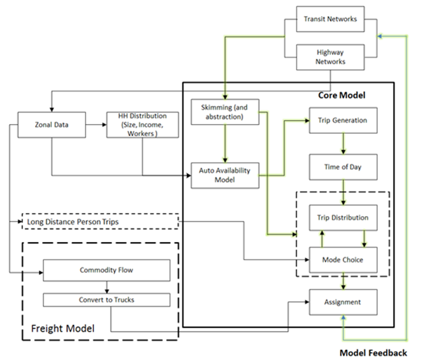
Source: ADOT, AZTDM3 Model Report, February 5, 2014

The AZTDM3 has five primary model components as described in the current model documentation:

• Setup and Skimming
• Household Models
• Person Travel
• Trucks/Long Distance
• Assignment

Setup and Skimming

By developing highway networks and updating the network settings, the AZTDM3 creates toll/non-toll skims using a generalized cost that is based on travel time, toll, and distance for the following four vehicle classes:

• Drive alone
• Shared ride 2
• Shared ride 3+
• Truck

Skimming is based on generalized cost (including monetary costs such as toll costs and non- monetary costs such as the cost of time) for a variety of travel characteristics.

Transit skims are created by developing transit networks, updating the transit network settings, and skimming based on highway, transit, and walk time for a variety of travel characteristics.

Transit abstraction methodology is used instead of traditional skimming to represent the local transit system. This methodology has been implemented in the California statewide travel demand model and is known as a hybrid transit abstraction method. The California model's coefficients were used as a starting point and then the AZTDM was calibrated to match the values of coded skims in Arizona network. The advantage of using this methodology instead of traditional skimming is that maintenance of the transit networks can be more easily facilitated.

Household Models

In this stage, trip generation is conducted for short-distance person trips only. Truck and long-distance person trips are processed separately in other stages of the model.

The base year for the model is 2010 and socioeconomic data have been updated from the AZTDM2. Trip generation rates for short-distance person trips were generated based on the 2009 NHTS. For each county, rates were calculated for five trip purposes:

• Home-based work (HBW)
• Home-based university (HBU)
• Home-based school (HBS)
• Home-based other (HBO)
• Non-home-based (NHB)

Person trip generation rates are stratified by area type. Area type definitions were calculated based on an accessibility measure. Area types used by the AZTDM3 include the following:

• Central Business District (CBD)
• Urban
• Suburban
• Rural
• Small Town Central Business District

The 2009 NHTS data were used for the estimation of the mode choice, auto availability, and time-of-day models. Public Use Microdata Sample (PUMS) data from 2006-2010 are used for calibrating the auto availability models.

The auto availability model was estimated for the following three alternatives:

• Household with zero vehicle
• Households with one vehicle
• Households with two or more vehicles

The outputs from the auto availability model are shares of zero, one, and two or more vehicle households and these are input into the trip generation model. A nested logit model is used for model estimation.

Short-Distance Mode Choice Models

The following modal alternatives are considered in estimating the mode choice models:

• Drive alone
• Shared ride 2
• Shared ride 3+
• Walk and drive access to local bus
• Walk, Drive, and Local Bus access to premium transit
• Non-motorized modes (Walk and Bike)

The AZTDM3 is a vehicle model; therefore, non-motorized choices are disabled during model calibration and application process.

Long-Distance Mode Choice Model

A nested logit model is used with an auto nest containing three alternatives (drive alone, shared ride2, and shared ride3+) and a transit nest containing drive and walk access. Air travel within Arizona is almost non-existent and is not considered in the model. The automobile drive alone is considered to be the base alternative. Model coefficients asserted from literature are shown in Table 1 (mainly Ohio statewide model^[1] and Florida High Speed Rail study^[2]).

Table 1: Proposed Variables in Long-Distance Mode Choice.

Time-of-Day Models

The time of day component in the AZTDM3 is moved upstream (compared to the AZTDM2) and the factors are applied to trips after the trip generation step. The factors based on trip purposes and mode (separate for Auto and Transit) are developed using the 2009 NHTS and are applied to produce the desired trip tables by purpose and time of day to be assigned to the network.

Person Travel

In this stage, the AZTDM3 performs trip distribution for short-distance person travel using a destination choice logit model. A multinomial logit model is then used to predict auto occupancy. Shares were derived from the NHTS and then smoothed to ensure a logical relationship among modes.

Truck & Long-Distance Person Travel

In this stage, the model separately processes short- and long-distance truck travel and long-distance person travel.

The short-distance truck model is a three-step model without mode choice. Its trip generation is segmented by 12 land use categories:

• Employer (start and end point of any truck trip)
• Retail
• Construction
• Farming
• Mining
• Households
• Governments
• Warehousing
• Transportation
• Office
• Industrial/Manufacturing

A gravity model is applied to distribute short-distance truck trips. Friction factors between zone pairs are calculated dynamically based on congested travel time.

Long-distance truck trips are processed by a Java program that uses a Transearch commodity flow matrix. Long-distance commodity flows are converted to truck trips using payload factors for single-unit and multi-unit trucks. An empty truck rate is used to factor the truck trips for returning empty trucks. Capacity and volume/delay function curve parameters were obtained from MAG. Passenger car equivalent (PCE) values were obtained from the Highway Capacity Manual (HCM 2000).

Long-distance person trips are mainly processed by a Java script, which reads and expands the 2002 NHTS long-distance data to a state-to-state trip table then disaggregated to TAZ using household data, employment, and a weighting scheme. A 10% sample of ticketed air travelers by BTS was also used. After missing NHTS records are synthesized and the NHTS data are expanded, trips are disaggregated to the AZTDM zones based on population and employment. The model also uses national and state parks as special attractions.

Assignment

Highway assignment in the AZTDM3 includes the assignment of auto trips to the highway network with preload of long-distance auto and truck trips as well as local bus vehicles by time of day. The assignment of trips onto the network is done by four time periods:

• AM Peak (6:00 a.m.-9:00 a.m.)
• Mid-Day (9:00 a.m.-3:00 p.m.)
• PM Peak (3:00 a.m.-6:00 p.m.)
• Night (6:00 p.m.-6:00 a.m.)

Highway assignment is implemented using user equilibrium assignment with mode and period specific tolls, PCEs, capacities, and preload volumes. Congested travel times are calculated using a BPR-type volume-delay function. The resulting assignments by time of day are summed into a daily table of assignment statistics by link. Long-distance auto and truck trips are assigned with All-or-Nothing (AON) assignment.

The model performs a feedback loop from trip generation to assignment. In the first feedback loop iteration, long-distance trips (person and truck) are loaded onto the network using an AON assignment. Then, the short-distance trips (person and truck) are loaded onto the network with a user equilibrium traffic assignment. Only the AM and MD travel times are fed back. Convergence is reached when the percent RMSE for the AM and the MD periods are both less than 1%. On the final model iteration, the model assigns PM and NT trips to a highway network.

For transit assignment, transit trips are assigned to the coded premium transit service routes (e.g., rail, BRT, express bus, and intercity routes) for walk, drive, and local bus access by time of day. The local bus vehicles are added to the preload volume in highway assignment and are not assigned in transit assignment. Transit assignment is based on the Pathfinder algorithm for transit networks created in the skimming procedures and origin-destination (O-D) transit trips for premium transit walk, drive, and local bus access.

Model Validation

Model calibration is focused on broad markets and the state highway system at the corridor level. Traffic counts were used to validate the AZTDM3.

Aggregate volume to count comparisons showed that the R-Square for the total flow was approximately 0.92, and the percent RMSE of total flow was 30% slightly above Ohio RMSE totals.

Figure 3: Total flow for the AZTDM3.

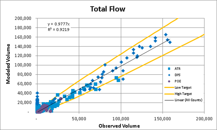
Figure 4: Percent RMSE by Volume Group-Total Vehicles.

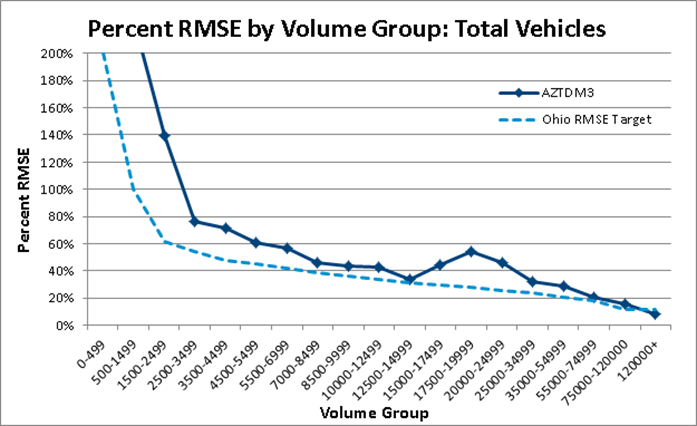
Source: ADOT, AZTDM3 Model Report, February 5, 2014

Screenline and cordon validations were also performed. The percent error of volume on 8 of 10 screenlines was within 20%. All screenlines and cordons were within maximum desired deviation.

Table 2: Screenline and cordon validations.

Screenlines Totals on Links with ATR Counts

Source: ADOT, AZTDM3 Model Report, February 5, 2014

Figure 5: Screenline locations in Arizona.

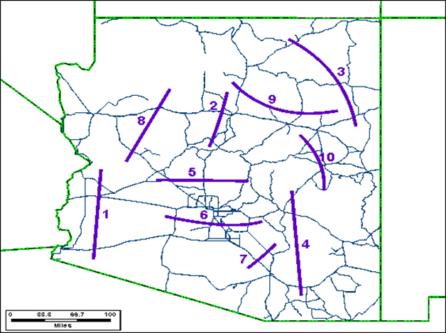
Screenlines Map

Source: ADOT, AZTDM3 Model Report, February 5, 2014

[1] Ohio DOT, Ohio Statewide Model, 2010.

[2] Wilbur Smith Associates and Steer, Davis, Gleave. Tampa - Orland High Speed Rail Ridership Study - Summary Report, November 2011.