
Chapter III. Methodology
Our analysis uses national travel survey data to examine four dimensions of intra-metropolitan travel:
- Personal miles traveled (PMT): the summed distance of all trips by all modes on the survey day;
- Activity participation (number of trips): the log of the number of trips made per day;
- Commute mode: the mode used for the longest (in terms of time) leg of an individual’s journey to work; and
- Social trip mode: the mode used for each social trip an individual makes, where social trips are defined in the surveys as trips “visiting friends or relatives” or trips for “other social or recreational” purposes.
The specific methodology we use to model each outcome measure varies. Therefore, in this chapter, we focus on elements of our methodology common across all four analyses.
A. Data
The U.S. Department of Transportation (DOT) periodically conducts a nationally representative travel survey of households. The survey includes a travel diary in which respondents provide details about mode, purpose, distance traveled, etc. for every trip on the survey day. Survey days include both weekdays and weekends. In addition, the survey includes a wealth of personal and household level data. In this study, we use data from 1990 Nationwide Personal Transportation Survey (NPTS), and the 2001 and 2009 National Household Travel Surveys (NHTS),8 as these three surveys correspond roughly with the 1990, 2000, and 2010 decennial censuses. We exclude respondents who live outside a Metropolitan Statistical Area (MSA), as well as respondents who made a single trip over 75 miles in length on the travel day.9
We had access to the confidential version of the two NHTS datasets (2001 and 2009), so for those two survey years we were able to supplement the datasets with census-tract level data from the U.S. Census on residential density. As we discuss below, the models also include a variable identifying the driver’s licensing regulation of the state in which the respondent lives.
B. Age Groups
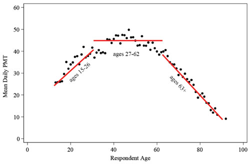
Because we are primarily interested in the activity participation of teens and young adults, we first had to develop a clear and defensible definition of that group. Unfortunately, scholars have not arrived at a consensus definition for teens and/or young adults—likely because no natural or obvious cutoffs exist for the wide range of phenomena (even within transportation scholarship) that one might wish to study. As such, we developed a technique to identify a reasonable break between a “teens and young adults” category and an “adult” category. Using average daily personal miles traveled (PMT) by age as a proxy for travel behavior and activity participation more generally, we employed an iterative cutoff-search technique that minimizes the root mean square error (RMSE) of regression line-fits for a number of age-based subsamples. We used the NHTS datasets from 2001 and 2009 to estimate appropriate cutpoints. As Figure 1 and Figure 2 show, the procedure determined an age classification system that grouped ages according to trends in PMT. Despite changes in absolute PMT between these two datasets, the cutpoints remained relatively stable. While the cutpoint search procedure suggested a cutpoint at 60/61 years in 2001, the procedure suggested a cutpoint of 62/63 in 2009. In this case, we simply split the difference and used a cutpoint of 61/62.
In three of our four analyses (trips, commute mode, and social trip mode), we use the following two age groups:
- Teens and young adults (ages 15–26, during which time PMT grows rapidly); and
- Adults (ages 27–61, during which time PMT remains relatively unchanged);
Figure 1: PMT Breakpoints, 2001 NHTS
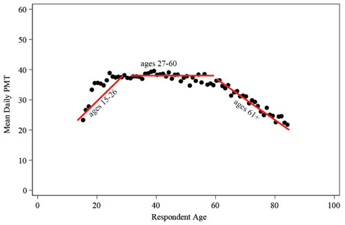
Figure 2: PMT Breakpoints, 2009 NHTS
For our analysis of personal miles traveled, we use three age groups: teens aged 15–18 (Group 1A), young adults aged 19–26 (Group 1B), and adults aged 27–61 (Group 2). Although there is no agreed upon definition of “teen” in the travel behavior literature, restricting our analysis to youth ages 15–18 has two advantages. First, this age group captures the transformational period for travel behavior when most teens obtain driver’s licenses. Second, travel decisions often take place at the household level and many young people begin to move away from home at age 19. In 2009, approximately 88 percent of respondents aged 15–18 lived with their parents, but at age 19 the figure fell to 74 percent and declines steadily thereafter with age.
C. Statistical Models
We construct a set of cross-sectional models using three years of data (1990, 2001, and 2009) to examine: (a) the determinants of travel, and (b) changes in these determinants over time. As noted above, the years chosen roughly correspond to a decade of change and the microdata data can be linked to census-tract level data from the decennial census and other supplemental data in a consistent manner. Drawing from the broader travel behavior literature, our models control for the major determinants of travel including variables that measure individual, household, neighborhood, and trip characteristics as well as the driver’s licensing regulations in the state in which the respondent lives.
In a separate set of models, we use the travel survey data to construct a set of quasi-cohort models. The NPTS and NHTS data are cross-sectional and are not samples of the same individuals over time. We, therefore, construct a set of pseudo-cohort models by linking observations across survey years by birth decade. Specifically, in each of these models (PMT, trips, commute mode, and social trip mode), we include data from all three survey years. Similar to the cross-sectional models, we control for the major determinants of travel behavior. To test whether cohorts that are more recent travel differently from prior cohorts, controlling for other factors, we introduce a series of decade-of-birth (cohort) variables. Figure 3 shows the ages of these birth cohorts for each of the three data years. This figure illustrates that, particularly for the most recent birth cohorts (1980s and 1990s), the observed behavior of that group only spans a limited range of life years. The 1990s birth cohort is included only in the 2009 dataset, and thus we interpret the coefficients associated with this birth decade with some caution. For instance, if the model suggests that those born in the 1990s have different travel patterns than those of other birth decades, this finding must be interpreted with the caveat that we have only provided the model with “overlapping” observations (of similar life years) for two other birth cohorts: those born in the 1970s and 1980s.
Figure 3: Ages of Cohorts Included in the Model by Data Year
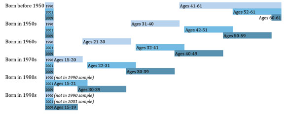
Table 5 shows the total number of person records in our model for each cohort across the three data years. While the 1990s birth cohort is the smallest of the six cohorts, it still contains over eleven thousand records. The largest cohorts in the study are those of participants born in the 1950s and 1960s, as these birth cohorts are not truncated at either end for any of the three data years.
| 1990 | 2001 | 2009 | Total | |
|---|---|---|---|---|
| Born before 1950 | 2,930 | 14,929 | 13,913 | 31,772 |
| Born in 1950s | 4,429 | 19,713 | 43,398 | 67,540 |
| Born in 1960s | 4,277 | 18,270 | 32,960 | 55,507 |
| Born in 1970s | 1,571 | 12,114 | 20,152 | 33,837 |
| Born in 1980s | 0 | 23,024 | 11,895 | 34,919 |
| Born in 1990s | 0 | 0 | 11,805 | 11,805 |
| Total | 13,207 | 88,050 | 134,123 | 235,380 |
D. Independent Variables
Although they vary in structure, the cross-sectional and cohort statistical models included in this analysis control for four, and for the mode split analyses five, categories of travel determinants:
- Individual characteristics,
- Household characteristics,
- Neighborhood characteristics,
- Driver’s licensing regulations, and
- Trip characteristics.
Table 6 summarizes the variables used in this analysis. Unfortunately, the NPTS/NHTS datasets do not include variables to measure some of our variables of interest. We also had difficulty incorporating external variables such as graduated driver’s licensing regulations.10 Therefore, in the text that follows, we discuss our construction of four of these variables: young adults living with parents, daily web use, graduated driver’s licensing regulations, and education.
| Variables | Definition |
|---|---|
| Individual Characteristics | |
| Age | Age |
| Sex | Female = 1, Male = 0 |
| Race/Ethnicity11 | Non-Hispanic Black, Non-Hispanic Asian, Non-Hispanic Other, Hispanic (omitted: Non-Hispanic White) |
| Foreign born | Not born in the United States |
| Employed | Yes =1, No = 0 |
| Web Use | Uses internet almost every day (Yes = 1, No = 0) |
| Driver | Driver =1, Non-Driver = 0 |
| Medical condition | Has medical condition making it hard to travel |
| Education |
For
adults (27–61): High School, Some College, College Graduate, Professional Degree
(omitted: less than HS) For youth (15–26): maximum education attained by any relative in household |
| Young Adult Lives with Parents | Lives with a parent and is between the ages of 19 and 26 |
| Household Characteristics | |
| Household Income | Log of household income |
| Number of adults | Number of adults |
| Number of children | Number of children |
| Childrearing responsibilities | Ratio of children to adults |
| Single parent | Single parent with at least one child under the age of 21 |
| Single family home | Lives in detached single house |
| Access to cars | Autos per adult in household; for social trips: number of autos in household |
| Neighborhood Characteristics | |
| Residential density | Log of census-tract residential population density |
| Large metropolitan areas | MSA > 3 million |
| New York | Lives in New York City |
| License Regulation Stringency | Lowest, Low, Medium, and High |
| Trip Characteristics | |
| Distance | Trip distance (in miles) |
| Commute time | Hours spent commuting on survey day (door to door) |
| Weekend travel | Trip on Saturday or Sunday |
| Peak period travel | Commute journey start time from 6:00 AM to 8:59 AM |
Young adult living with parents: This variable captures the potential effect of a “boomerang lifestyle—returning to live with one’s parents after a period of living apart—on youth travel behavior. The variable is dichotomous, taking a value of “1” if the respondent lives with a parent and is between the ages of 19 and 26. This is an imperfect measure because it does not distinguish between young people who have returned home and young people who never left the home in the first place. To minimize the risk of including youth who have not yet left the home, we do not include people younger than 19 in this variable.
Daily Web Use: This variable is also dichotomous and takes a value of “1” if the respondent uses the internet “almost every day.” Youth who use the web daily may travel less than their peers who use the web less frequently if web use is a substitute for travel. Conversely, we expect web use to increase travel for youth if it is a complement. The 1990 NHTS did not include questions regarding web use. We assume daily web use was virtually non-existent in 1990, particularly for youth.
Licensing Regulations: Graduated drivers licensing (GDL) regulations typically include some combination of components to phase in driving privileges, including minimum permit age, required hours of supervised driving, restrictions on nighttime driving, and restrictions on driving with passengers. In general, states have gradually ratcheted up their GDL regulations over the past two decades. For this research, we used the GDL Ranking system developed by the Insurance Institute for Highway Safety (IIHS), which many traffic safety researchers use to assess safety outcomes of GDL regulations. We include the criteria for the IIHS rating system in Table 7 below.
We applied the rating system to historical licensing information provided by Federal Highway Administration (FHWA) for 1990, and the IIHS for the years 1995 to 2009 (U.S. Department of Transportation, 1992; Sims, 2012). Neither of these two sources provides complete license information for all three years (1990, 2001, and 2009). The FHWA data only include states with license regulations specifically for juveniles. As a result, 23 states do not appear in the data. Accordingly, we assumed the lack of juvenile specific regulations was equivalent to having a GDL poor ranking. The IIHS data did not contain information on regulations in Massachusetts, New Jersey, or Washington DC. We used 2011 data and information about implementation dates to determine license regulations in 2009, which we use as a proxy for the 2008 figures in these three locations. We were unable to estimate the level of licensing restrictions in those states in 2000.
Wherever possible we followed the standard of the safety literature by using the licensing information for the year preceding the year of interest. In other words, for analysis of travel behavior in 2009 we used the licensing requirements that were in effect in 2008. This step is necessary because many states do not retroactively apply restrictions to young drivers who have already received a license. Therefore, a driver who received a license at the beginning of 2009 would not be subject to restrictions if tougher laws came into effect later in the calendar year. Unfortunately, we could not secure licensing information for 1989. However, we are confident that licensing regulations were not yet undergoing dramatic changes and that our 1990 information accurately reflects the state of licensing regulations in 1989. Based on the IIHS point system, we categorized state driver’s licensing regulations from least to most stringent—lowest (< 2 points), low (2-3 points), medium (4-5 points), and high (6+ points).
| Component | Specific Restriction | Points |
|---|---|---|
| Learner’s Phase | ||
| Minimum permit age | 16 or older | 1 |
| Minimum permit age | Less than 16 | 0 |
| Permit holding period | 6 or more months | 2 |
| Permit holding period | 3-5 months | 1 |
| Permit holding period | Less than 3 months | 0 |
| Required practice hours | 30 or more hours | 1 |
| Required practice hours | Less than 30 hours | 0 |
| Intermediate Phase | ||
| Restriction on night driving | 10 pm or earlier | 2 |
| Restriction on night driving | After 10 pm | 1 |
| Restriction on night driving | No restriction | 0 |
| Restriction on underage passengers | Zero or 1 passenger | 2 |
| Restriction on underage passengers | 2 passengers | 1 |
| Restriction on underage passengers | 3 or more passengers | 0 |
| Duration of night driving restriction | 12 months or more | 1 |
| Duration of night driving restriction | Less than 12 months | 0 |
| Duration of passenger restriction | 12 months or more | 1 |
| Duration of passenger restriction | Less than 12 months | 0 |
| IIHS Graduated Licensing Rating* |
IIHS Graduated License Stringency |
|
| Good | High | 6+ points |
| Fair | Med | 4-5 points |
| Marginal | Low | 2-3 points |
| Poor | Lowest | < 2 points |
Education: This variable takes five possible values: Less than a High School Degree, High School Graduate, Some College, College Graduate, and Professional Degree. In the regression models that follow, “Less than High School” is the omitted category. Educational attainment is self-reported in the NHTS. Measuring adult educational attainment is straightforward, but measuring education for youth is more complicated. Educational attainment for people 15 to 26 is highly correlated with age. Moreover, there is no clear way to establish whether a 17-year-old without a high school degree will complete a high school degree in the coming year. In this research, we assume parent’s education is a better predictor of future educational attainment than current educational attainment for youth. Therefore, for each young person we created a variable representing the educational attainment of their parent by assigning the value of the maximum education attained by any relative in their household.
E. Missing Data
The travel surveys differ slightly from year to year, complicating multi-year comparisons considerably. Nevertheless, to the greatest extent possible, the following analyses contain variables that are identical across the three survey years. As Table 8 shows, within a given survey year, some questions were only asked of respondents of a certain age. For example, in 2001 and 2009, respondents aged 15 were not asked about their use of the internet or their employment status, but respondents over age 16 were asked those questions. Similarly, in 1990, respondents aged 15 were not asked about their driver status, while their older peers were. Yet in many states, 15-year-olds are allowed to drive with permits. Fortunately, we were able to infer some information about these variables from other questions in the survey, which we detail below.
Employed: If a 15-year-old indicated a trip purpose that was a commute or a work-related trip on their travel day, we coded them as employed. This method inevitably misses many workers, particularly because youth have irregular work schedules. The correlation between actual work status and an identically constructed estimate of work status for 16, 17, and 18-year-olds in 2009 was .19, .39, and .53, respectively. So while we were able to correctly add worker information for some 15 year-olds using this method, others are unavoidably missing information.
Driver Status: To estimate driver status in 1990, we used information about which family member drove on a given trip. If a 15-year-old indicated their own ID number for any trip, we considered them a driver.
Daily Web Use: One of the hypotheses we wished to test was whether the use of information technologies can help explain a reduction in the trip making, PMT, and/or automobile use among youth. However, while the 2001 and 2009 NHTS include a number of questions related to the use of the internet, the datasets do not include these data for individuals aged 15 or younger. Because we wished to include 15-year-olds in our models, we opted to use a multiple imputation strategy to estimate internet usage for 15-year-olds.
Multiple imputation is a method for “filling in” missing data in a dataset by using the existing, non-missing data to uncover patterns that predict the outcome of interest, and then using these predictive models to estimate probable values for the missing data.12 The imputation strategy is “multiple” in that it uses a Monte Carlo estimation technique to create multiple probable outcomes for each missing value. For instance, if the predictive model estimates that an individual has a 51 percent chance of using the internet on a daily basis, the multiple imputation technique would create 10 random but probable records for that individual; in roughly five of those records, the individual would be coded as using the web daily. These records are then used in a series of estimation models that are then averaged together to obtain a final model that accounts for the missing data in a principled fashion.
Education: Similarly, educational attainment is not available for all ages in all datasets. For instance, in the 2009 dataset, educational attainment is only available for individuals age 18 and older. However, this does not present a challenge to our models because we hypothesized that, for school-age youth, the individual level of educational attainment should matter less than the parent’s level of education. Thus, we used the highest level of education achieved by any member of the household for youth in many of our models.
| Ages 15 |
Ages 16 |
Ages 17 |
Ages 18 |
|
|---|---|---|---|---|
| 1990 | ||||
| Employed | Missing Data |
Data Available |
Data Available |
Data Available |
| Driver Status | Missing Data |
Data Available |
Data Available |
Data Available |
| Web Use | Missing Data |
Missing Data |
Missing Data |
Missing Data |
| Education | Data Available |
Data Available |
Data Available |
Data Available |
| 2001 | ||||
| Employed | Missing Data |
Data Available |
Data Available |
Data Available |
| Driver Status | Data Available |
Data Available |
Data Available |
Data Available |
| Web Use | Missing Data |
Data Available |
Data Available |
Data Available |
| Education | Missing Data |
Data Available |
Data Available |
Data Available |
| 2009 | ||||
| Employed | Missing Data |
Data Available |
Data Available |
Data Available |
| Driver Status | Data Available |
Data Available |
Data Available |
Data Available |
| Web Use | Missing Data |
Data Available |
Data Available |
Data Available |
| Education | Missing Data |
Missing Data |
Missing Data |
Data Available |
9Table 48 in the appendix shows the number and percentage of trips by length and survey year.
10We were also interested in controlling for the unemployment rate of the metropolitan area in which respondents lived. Unfortunately, the NHTS/NPTS surveys do not identify metropolitan areas for respondents who live in areas with populations of less than one million. To attach metropolitan unemployment rates, we would have had to omit data for over 330,000 trips that occur in MSAs smaller than 1 million.
11In the NPTS and NHTS datasets, race/ethnicity data exist only for the household respondent, the individual who interacts with the telephone survey worker. Thus, this is an imperfect measure of the race/ethnicity of the individual.
12For a thorough treatment, see Rubin (1987) and Schafer (1999).