
Chapter VI. Activities/Trips
A. Introduction
Except for walks in the park and cruising on a Saturday night, travel is a means to an end. Economists describe the demand for travel as “derived” because people travel in order to access other things—work, shops, restaurants, friends, and so on. One stands on a crowded subway each morning not for the thrill of the ride, but to get to work on time; one searches for a parking space at the grocery store not for the joy of finding an open space, but to stock one’s house with food. Transportation is often a critical link to education, paid work, recreation, health care, culture, and many other aspects of quality living. While PMT is an excellent measure of mobility, it does not tell us much about access, or the utility of personal travel. To examine travel utility or access, we must turn our attention to the purpose of trips.
Trip-making is an excellent, albeit indirect and understudied window on activity participation. People’s work habits, shopping behavior, recreational preferences, and so on are revealed by the stated purpose of their travel in surveys like the NPTS and NHTS.
However, all things are rarely equal. There are but 24 hours in a day and more time spent stuck in freeway traffic or waiting a long time for a bus or train reduces the number of activities that can be enjoyed at the ends of trips. A few long or expensive trips tend to reduce the total number of trips one can make in a day. Conversely, physical proximity to destinations and access to information and communications technologies can reduce the time spent traveling or the need to make trips at all. In a compact, mixed-use area, a drive to the store can be replaced by a short walk, or travel to a meeting with colleagues can be replaced by Skype. But do such opportunities affect the number, type, and mix of trips people make? If so, will such changes in trip-making patterns be more apparent among teens and young adults than among older adults? These questions motivate the analysis that follows.
B. Methodology
To analyze patterns and trends of trip-making among teens and young adults, we again rely on the 1990 Nationwide Personal Transportation Survey and the 2001 and 2009 National Household Travel Surveys of metropolitan residents making trips of less than 75 miles on the survey day. Our variable of interest is the number of activities in which teens and young adults participated per day across all three survey years. Unlike the PMT analysis, where we split youth into two categories (teens and young adults) and ran three separate models for all three years, this analysis compares two groups of travelers: youth (ages 15–26) and adults (ages 27–61).
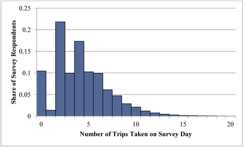
Because the number of trips made by individuals is considerably right-skewed (Figure 16), with a small number of individuals making a large number of daily trips, we use a log-transformed version of the variable in our models. A sizeable share of respondents (roughly 10 percent in each of the datasets) did not make any trips during the survey day. Because the log(0) is not defined, we also add a trivial amount to the variable before log transforming it.
Figure 16: Number of Daily Trips (2009)
Following Lu and Pas (1999), we employ a structural equation model (SEM) as described by Bollen (1989). Structural equation models employ a maximum-likelihood technique for estimating model parameters, though they differ from other models in one important way. Unlike more common linear regression models employed in the previous chapter that posit a relatively simple linear causality, SEM allows the researcher to hypothesize complex causal relationships that involve multiple intermediary processes, which are simultaneously specified. SEMs effectively allow us to specify sub-models that then relate to one another in a larger modeling context.
Many SEMs incorporate elements of factor analysis to explore the influence of latent (unmeasured and unmeasureable) variables on variables of interest. While this is a very common component of structural equation models, we do not employ it here, as our hypothesized causal pathways do not suppose latent variables, but rather rely on more direct and measureable relationships (such as the relationship between income and car ownership).
Figure 17: Simplified Overview of Structure Equation Models (SEMs)
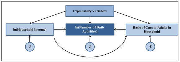
We estimate our SEMs using the Stata 12.1 statistical software package. Figure 17 presents a simplified overview of the model’s structure. The SEM procedure estimates three sub-models: first, a model of household income estimated using a set of explanatory variables that include race/ethnicity, education, worker status, whether the respondent has a medical condition, the respondent’s neighborhood residential density, and whether the respondent is a single parent or the child of a single parent. This model of income feeds into a model of car ownership (to the far right of the diagram). Here, the ratio of cars to adults in the household is modeled as a function of household income (sub-model 1), as well as a number of other explanatory variables (race/ethnicity, household size, and the neighborhood residential density). Both of these sub-models then feed into the model of daily activity participation, to which we add additional explanatory variables. These additional explanatory variables include those used in the previous sub-models, as well as the respondent’s age, sex, foreign-born status, web usage, and commute duration. The advantage of such a nested, structured approach to modeling daily activity participation is that the researcher hypothesizes and then specifies the specific causal pathways thought to influence a particular outcome. SEM, then, is a way to estimate empirically the relative weight and robustness of these pathways.
We then constructed the same set of related SEM sub-models—to predict auto access (ratio of autos to adults), income, and activities—in a multi-survey-year format similar to the quasi-cohort model in the PMT analysis above. For each model, we include records from all three survey years for the usual array of explanatory variables, as well as both a variable noting the survey year, and in the auto access and activities models we also included variables for the decade of birth of each respondent.
C. Descriptive Statistics
As with our discussion of PMT, people tend to make more trips as they age. As Figure 18 illustrates, using the 2009 NHTS, the mean number of trips made per day varies considerably by age. The youngest individuals in our sample (age 15) made an average of just over three trips per day in 2009, while individuals in their mid-40s made almost 1.5 times as many trips (4.5).
Figure 18: Mean Number of Trips by Age (2009)
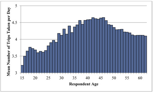
Figure 19 shows that there have been significant changes over time in the activity participation patterns of various age groups. While older individuals in the 1990 survey report making more trips in the 2001 survey, and more trips again in the 2009 survey, the story for teens and young adults is very different. In 2009, teens and young adults reported making fewer trips than in 2001.21
Figure 19: Mean Number of Daily Trips by Age and Year (1990, 2001, and 2009)
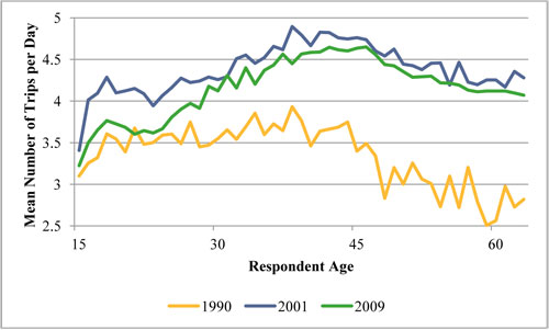
Figure 20 shows the mean number of trips taken by our two age groups of interest for the three data years. This figure illustrates that both adults’ and youths’ trip-making decreased from 2001 to 2009, but that the decrease was considerably more pronounced for youth than for adults.
Figure 20: Mean Number of Daily Trips by Age and Year (1990, 2001, and 2009)
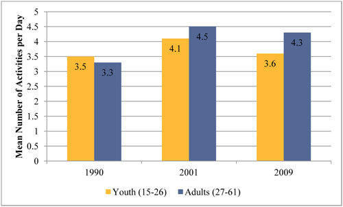
Figure 21 shows the difference between 2001 and 2009 trip-making rates. The graph shows considerable variation, though a trend is apparent—the greatest decline in trip-making has occurred among young people. In fact, those in their late teens were, on average, making 0.5 fewer trips per day in 2009 than the same age group did in 2001.
Figure 21: Difference in Trip-Making by Age (2001 to 2009)
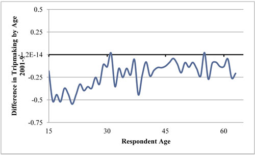
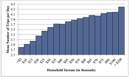
Figure 22 shows the relationship between household income and trip-making. At the lower end of the income distribution, an increase in household income is associated with rapid gains in trip-making. For instance, while those making $5,000 to $10,000 per year make, on average, just 2.9 trips per day, those earning more than $10,000 per year make 3.25 trips on average—an increase of 12 percent.
On the higher end of the income spectrum, more income is still associated with higher levels of trip-making, but the effect is milder. Why? First, income is an enabler of activities, many of which (e.g., shopping and other recreational activities) have a monetary cost associated with them.
Figure 22: Household Income and Trip-Making (2009)
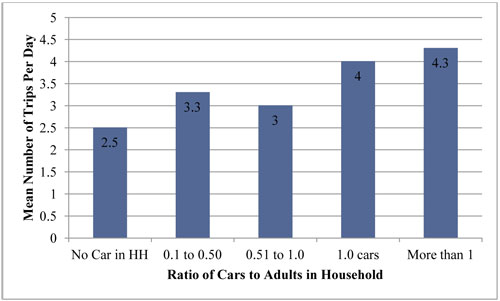
Second, and more importantly, our analysis of personal travel shows that automobile access is a strong predictor of PMT. Because income enables car ownership and use, we would expect that those with incomes sufficient to pay for cars would tend to travel more miles, and indeed that is the case. But once one has access to a private vehicle for travel, additional income (and more auto access) is less likely to stimulate additional travel because one can only drive one car at a time. As with personal travel, we expect that greater access to automobiles will be associated with more trips. In most places in the United States, the automobile is the most convenient mode of transportation for accessing activity sites, particularly those offering abundant free parking. As such, we anticipate that those households with less than one car per adult will make, on average, fewer trips than will households with one or more cars per adult.
Figure 23 shows the relationship between auto availability and trip-making. While the relationship between auto availability and trip-making does not progress monotonically according to our expectations, in general, those with one or more cars per adult make considerably more trips (3.5 trips or greater) than those with fewer cars; those with no car make, on average, one trip less per day (2.5 trips) than those with one car per adult.
Figure 23: Auto Availability and Trip-Making (2009)
D. Cross-Sectional Model and Model Results
Table 22 shows the results of six structural equation models of activity participation for youth and adults across the three (1990, 2001, and 2009) datasets. The control variables largely conform to expectations drawn from the extensive travel behavior literature. This section describes the sub-models, and the following section describes the results for our relationships of interest.
| Youth 1990 |
Youth 2001 |
Youth 2009 |
Adult 1990 |
Adult 2001 |
Adult 2009 |
|
|---|---|---|---|---|---|---|
| Submodel: Ratio of Cars to Adults in HH | ||||||
| Individual Characteristics | ||||||
| NH White | omitted | omitted | omitted | omitted | omitted | omitted |
| NH Black | -0.22*** |
-0.18*** |
-0.13*** |
-0.14*** |
-0.11*** |
-0.08*** |
| NH Asian | n/a | -0.14*** |
-0.04* |
n/a | -0.13*** |
-0.10*** |
| Hispanic | -0.12*** |
-0.14*** |
-0.03* |
-0.04** |
-0.08*** |
-0.05*** |
| NH Other | -0.04 | -0.08* |
-0.03 | -0.04 | -0.05** |
0.003 |
| Household Characteristics | ||||||
| Household Income (ln) | 0.21*** |
0.15*** |
0.19*** |
0.16*** |
0.14*** |
0.14*** |
| Number of Adults | -0.16*** |
-0.10*** |
-0.12*** |
-0.15*** |
-0.13*** |
-0.13*** |
| State Licensing Regulations | ||||||
| Stringency: Lowest | omitted | omitted | omitted | omitted | omitted | omitted |
| Stringency: Low | -0.13*** |
0.01 | -0.18* |
-0.07*** |
0.01 |
-0.08** |
| Stringency: Medium | n/a | -0.03 | -0.16* |
n/a | 0.002 | -0.14*** |
| Stringency: High | n/a | 0.04** |
-0.15 | n/a | 0.07*** |
-0.12*** |
| Geographic Characteristics | ||||||
| Population Density (ln) | -0.06*** |
-0.08*** |
-0.07*** |
-0.06*** |
-0.08*** |
-0.06*** |
| Constant | -0.70*** |
-0.29*** |
-0.60*** |
-0.23*** |
-0.14*** |
-0.03 |
| Youth 1990 |
Youth 2001 |
Youth 2009 |
Adult 1990 |
Adult 2001 |
Adult 2009 |
|
|---|---|---|---|---|---|---|
| Submodel: In(Household Income) | ||||||
| Individual Characteristics | ||||||
| NH White | omitted | omitted | omitted | omitted | omitted | omitted |
| NH Black | -0.27*** |
-0.52*** |
-0.67*** |
-0.31*** |
-0.45*** |
-0.44*** |
| NH Asian | n/a | -0.36*** |
-0.36*** |
n/a | -0.19*** |
-0.05*** |
| Hispanic | -0.47*** |
-0.79*** |
-0.81*** |
-0.33*** |
-0.53*** |
-0.37*** |
| NH Other | -0.08 | -0.15** |
-0.41*** |
-0.25*** |
-0.19*** |
-0.19*** |
| Employed | 0.23*** |
0.09** |
-0.001 | 0.28*** |
0.25*** |
0.28*** |
| Medical Condition | n/a | -0.29*** |
-0.23** |
n/a | -0.44*** |
-0.46*** |
| Less than High School | omitted | omitted | omitted | omitted | omitted | omitted |
| High School Graduate | -0.27*** |
-0.12 | -0.11*** |
0.51*** |
0.23*** |
0.71*** |
| College Graduate | -0.13** |
-0.01 | 0.10 | 0.92*** |
0.60*** |
1.26*** |
| Household Characteristics | ||||||
| Number of Adults | 0.21*** |
0.13*** |
0.10*** |
0.25*** |
0.09*** |
0.13*** |
| Single Parent | -0.96*** |
-0.57*** |
-0.95* |
-0.45*** |
-0.57*** |
-0.54*** |
| Child of a Single Parent | -0.10 | n/a | -0.88 | n/a | n/a | n/a |
| Constant | 9.93*** |
10.41*** |
10.98*** |
9.31*** |
10.28*** |
9.87*** |
| Youth 1990 |
Youth 2001 |
Youth 2009 |
Adult 1990 |
Adult 2001 |
Adult 2009 |
||||
|---|---|---|---|---|---|---|---|---|---|
| Submodel: In(Activities on Survey Day) | |||||||||
| Individual Characteristics | |||||||||
| Age | -0.01*** |
-0.01 | 0.01 | -0.005*** |
<0.001 | 0.003*** |
|||
| Female | 0.07*** |
0.06*** |
0.08*** |
0.10*** |
0.04*** |
0.06*** |
|||
| NH White | omitted | omitted | omitted | omitted | omitted | omitted | |||
| NH Black | -0.07** |
-0.03 | 0.01 | -0.04** |
-0.03 | 0.01* |
|||
| NH Asian | n/a | -0.001 | 0.003 | n/a | -0.10*** |
-0.09*** |
|||
| Hispanic | -0.09** |
-0.09** |
0.03 | -0.06** |
0.01 | 0.03*** |
|||
| NH Other | -0.03 | 0.01 | 0.10 | -0.20*** |
-0.02 | -0.03** |
|||
| Immigrant | n/a | -0.09** |
-0.02 | n/a | -0.06*** |
-0.03*** |
|||
| Employed | 0.12*** |
0.20*** |
0.24*** |
-0.01 | 0.08*** |
0.10*** |
|||
| Uses Internet Daily | n/a | 0.03 | 0.02 | n/a | 0.03*** |
0.08*** |
|||
| Medical Condition | n/a | -0.25*** |
-0.14** |
n/a | -0.21*** |
-0.25*** |
|||
| Hours Spent Commuting | -0.11*** |
-0.07 | -0.13*** |
-0.09*** |
-0.08*** |
-0.08*** |
|||
| Less than High School | omitted | omitted | omitted | omitted | omitted | omitted | |||
| High School Graduate | 0.09*** |
0.21** |
-0.01 | 0.08*** |
0.11*** |
0.06*** |
|||
| College Graduate | 0.08* |
0.10*** |
0.02 | 0.13*** |
0.12*** |
0.16*** |
|||
| Household Characteristics | |||||||||
| Household Income (ln) | -0.04*** |
-0.02 | 0.03** |
0.04*** |
0.06*** |
0.04*** |
|||
| Number of Adults | -0.03** |
-0.003 | -0.04*** |
-0.05*** |
-0.02** |
-0.02*** |
|||
| Single Parent | 0.18* |
-0.01 | 0.21 | 0.0004 | 0.08*** |
0.06*** |
|||
| Child of a Single Parent | 0.11** |
n/a | 0.03 | n/a | n/a | n/a | |||
| Ratio of Children to Adults | -0.06*** |
0.00 | 0.01 | 0.04*** |
0.09*** |
0.13*** |
|||
| Autos Per Adult | 0.05** |
0.08*** |
0.10*** |
0.06*** |
0.05*** |
0.03*** |
|||
| State Licensing Regulations | |||||||||
| Stringency: Lowest | omitted | omitted | omitted | omitted | omitted | omitted | |||
| Stringency: Low | -0.03 | 0.03 | -0.13 | -0.06*** |
0.05*** |
-0.08 | |||
| Stringency: Medium | n/a | 0.02 | -0.18 | n/a | 0.02** |
-0.13** |
|||
| Stringency: High | n/a | 0.02 | -0.13 | n/a | 0.04** |
-0.12** |
|||
| Geographic Characteristics | |||||||||
| Population Density (ln) | -0.001 | 0.000 | 0.01* |
0.004 | 0.01** |
0.02*** |
|||
| Constant | 1.89*** |
1.31*** |
0.69*** |
0.97*** |
0.46*** |
0.56*** |
|||
| Youth 1990 |
Youth 2001 |
Youth 2009 |
Adult 1990 |
Adult 2001 |
Adult 2009 |
|
|---|---|---|---|---|---|---|
| Variance | ||||||
| Var (Ratio of Cars to Adults) | 0.21 | 0.17 | 0.18 | 0.19 | 0.22 | 0.23 |
| Var (ln(Household Income)) | 0.81 | 0.81 | 0.89 | 0.51 | 0.59 | 0.60 |
| Var (ln(Activities on Survey Day) | 0.30 | 0.40 | 0.39 | 0.27 | 0.42 | 0.42 |
| N | 4,343 | 12,305 | 20,249 | 11,649 | 59,682 | 115,401 |
| R Square (Overall) | 0.32 | 0.34 | 0.34 | 0.34 | 0.37 | 0.38 |
| KEY: |
|---|
| Statistically Significant |
| Statistically Significant Over Time (across all the years for which data were available) |
E. Income and Auto Availability Submodels
The broader travel behavior literature suggests that two major drivers of activity participation are income and auto ownership (Lu and Pas, 1999; Farber and Paez, 2009). We designed our models to incorporate these two variables as submodels within the larger structural equation model. We expect that greater household income and greater auto availability will increase activity participation for youth and adults; we also expect income to have an independent effect on car ownership.
The models suggest that income, in addition to having a strong direct effect on activity participation, also has an indirect effect through the mediating variable of auto ownership. However, the results do not consistently conform to our expectations. For youth in 1990 and 2001, greater household income has a negative direct effect on activity participation (trip-making), and strong positive effect on auto ownership. This means that, for youth, the effect of income on trip-making is due to the enabling of auto access, and not to the facilitation of trips in other ways (such as by providing money to spend at the trip end). Because auto ownership has a strong positive effect on trip-making, the income and auto access variables must be considered in concert with one another rather than separately. Table 23 shows these relationships.
In all but the 1990 youth model, the combined effect of income on trip-making is positive. To help illuminate the magnitude of these changes, we provide an illustrative example drawing on the data presented in Table 23 on the combined direct effects of income on trip-making. An increase in income from $20,000 to $30,000, for instance, would result in a 0.41 unit change in the log-transformed income of the household. This, in turn, would result in a -0.012 (or 0.41 × -0.029) reduction in the log-transformed number of trips the model expects youth to make in 1990. This reduction means a very slight reduction in the number of actual trips—just over a one percent reduction (a multiplicative effect of 0.988, or exp(-0.012)). For adults in the same year, we would expect the same change in income to result in an increase of 2.1 percent in trip-making, slightly more than the reduction we see among youth. For all other models, we see a positive relationship between income and trip-making, though the effect is moderate.
| Youth (15–26) 1990 |
Youth (15–26) 2001 |
Youth (15–26) 2009 |
Adults (26–61) 1990 |
Adults (26–61) 2001 |
Adults (26–61) 2009 |
||
|---|---|---|---|---|---|---|---|
| a | Direct Effect of Income (ln) on Trips (ln) | -0.039 | n.s. | 0.026 | 0.043 | 0.06 | 0.037 |
| b | Direct Effect of Income (ln) on Auto Availability | 0.21 | 0.153 | 0.194 | 0.156 | 0.14 | 0.143 |
| c | Direct Effect of Auto Availability on Trips (ln) | 0.049 | 0.08 | 0.098 | 0.058 | 0.049 | 0.033 |
| d | Indirect Effect of Income (ln) on Trips (ln) (b × c) | 0.01 | 0.012 | 0.019 | 0.009 | 0.007 | 0.005 |
| e | Total Effect of Income (ln) on Trips (ln) (a + d) | -0.029 | 0.012 | 0.046 | 0.052 | 0.067 | 0.041 |
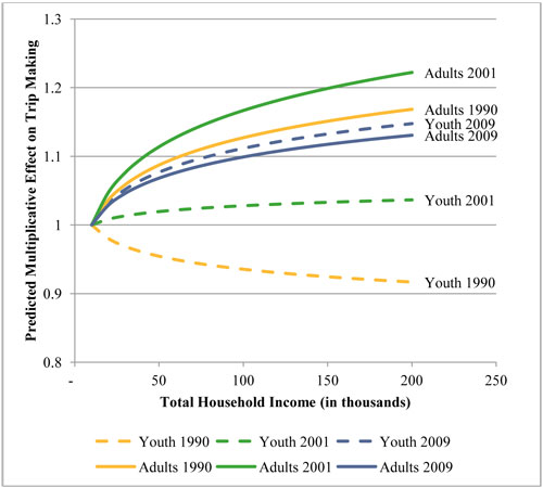
Figure 24 provides a graphical representation of the expected effect of income on trip-making for youth and adults for all three periods. Income appears to influence adults’ trip-making more than youth’s trip-making. However, for the 2009 model, the difference between the youth effect and the adult effect is not meaningful, mostly due to the waxing importance of household income in predicting youth trip-making and activity participation. While the effect of income has grown in importance for youth over time, the models suggest that the effect of income declined considerably for adults between 2001 and 2009. We hypothesize that this trend reflects the effects of the recession on households whose activity patterns were constructed prior to the economic downturn. By examining Table 23, we can see that the indirect effect of income (i.e., the effect of income on auto ownership) remained relative constant across the three time periods for adults, while its direct effect declined sharply. This, combined with a weakened effect of auto availability on trip-making, suggests that while income continued to play a large role in determining auto access, the other effects of income on trip-making are waxing for youth and waning for adults.
Figure 24: Overview of Expected Effect of Income on Trip-Making, Youth and Adults, Household
Income of $10,000 Base (=1.0) (1990, 2001, and 2009)
Automobile availability, independent of income effects, also has a significant positive influence on trip-making. Our model suggests that, for a two-adult household, an increase from one car (0.5 cars per adult) to two cars (1.0 cars per adult) would result in an increase of log-transformed trip-making of 0.025 for youth in 1990, and nearly 0.05 for 2009. This means that the availability of cars led youth to make over 2.5 percent (exp(0.025)) more trips in 1990, and over 5 percent more trips in 2009—a relatively strong effect. Further, our models show that, for youth, the importance of auto availability in determining trip-making has grown over time, while the effect has diminished for adults over the same period.
Worker Status. Being employed is, of course, highly correlated with income. But beyond the income effects of working, the models collectively suggest that employed people consistently take significantly more trips per day than non-working individuals, and this is particularly true for youth. While the adult models suggest a moderate direct influence of being employed on trip-making (no effect in 1990, roughly 8 percent more trips in 2001, and 10 percent more trips in 2009), the effect on youth is considerably stronger, growing from roughly 12 percent (exp(0.121)) more trips in 1990 to nearly 27 percent (exp(0.239)) more trips in 2009. At the same time, working youth’s contribution to overall household income has diminished substantially, from a strong effect in 1990 (a 26 percent increase in household income) to having no statistically significant effect on household income in 2009; this may be due to the fact that youth employment has declined the most in lower income households where their employment has the largest effect on overall household income. For adults, worker status is a strong and significant determinant of total household income across all three periods.
While being a worker has a positive influence on trip-making, as expected, the duration of one’s commute has a countervailing effect. For youth, we observe a roughly 12 percent decrease in the number of trips taken for each additional hour of commuting in 1990 and 2009; for 2001, the model finds no effect. Commute duration appears to influence adults’ activity patterns as well, but to a lesser degree. In all three adult models, we find a roughly 8–9 percent decrease in daily activities for each additional hour spent commuting. The data suggest that adults’ days consist of more shopping trips and fewer social/recreational trips. Thus, it is likely that adults’ trips are less discretionary, making it harder for adults to omit a trip when their commutes are long.
Web Use. Similar to our analysis of PMT, the SEM trip-making models presented here do not provide any strong evidence that internet usage has an influence—either positive or negative—on trip-making. In the 2001 and 2009 models (web usage is not available in the 1990 dataset, but we can presume that it was near zero for most people), daily internet usage has no statistically significant influence on the number of trips that youth make. For adults, only the 2009 model suggests a relationship, though a positive one. Specifically, the model suggests that adults who use the internet daily take, on average, 8 percent (exp(0.078)) more trips per day than do those adults who do not use the internet daily, controlling for other factors. This, too, is congruent with the findings in our PMT analysis, and suggests that any effect that web use has as a substitution for travel is more than offset by the fact that those who access the web daily are inclined to engage in more activities than those who do not. This weak substitution effect is consistent with the literature on information and communications technologies and travel more broadly (Kwan 2006; Taylor 2011).
Licensing Restrictions. Similarly, the models suggest that the increasingly strict drivers’ licensing laws in the United States have had a modest influence at best on youth activity participation. All three models for the youth age group find no evidence of a direct relationship between licensing restrictions and the number of activities per day. Although the models may point to a dampening effect on the number of automobiles a household purchases, these coefficients are not consistent across the three model years. At most, the models predict a reduction of less than 0.20 cars per adult in the household when licensing restrictions become stricter. However, these coefficients are only marginally significant for 2009, and the 2001 model shows a countervailing effect—suggesting that, in 2001, stricter licensing regimes were associated with more, and not less, trip-making.
Why, given that auto access is so strongly associated with trip-making, do stricter teen licensing requirements appear not to be depressing youth activity participation? The possible explanations are many, and beyond the scope of this analysis to carefully scrutinize. However, we hypothesize that possible explanations might include that youth are simply traveling more via other modes, being chauffeured more by parents and friends, or ignoring driving restrictions. We discuss this issue further in the conclusion of this report.
Control Variables of Note. The effect of race/ethnicity on trip-making patterns appears to be diminishing over time. In general, we observe that people of color make fewer trips than their white counterparts do, although the effect has diminished considerably. This finding is consistent with the literature on race/ethnicity and travel generally (Farber and Paez, 2009). Our models suggest that race and ethnicity play a larger direct role in determining adults’ trip-making than youth’s trip-making. However, for youth and adults alike, race/ethnicity plays a role in determining income, which in turn influences trip-making. In the 2009 models, race/ethnicity plays no statistically significant direct role in determining youth’s trip-making rates, and the influence of race/ethnicity on income has diminished considerably over the 19-year period analyzed in our models. Similarly, for adults we see that the magnitude of the direct effect of race/ethnicity on trip-making has diminished considerably over time, as has the effect of race/ethnicity on income. However, this diminishing pattern does not hold for Hispanic adults across all three models.
F. Quasi-Cohort Models and Model Results
Table 23 shows the results from the same set of related SEM submodels using a multi-survey-year format similar to the cohort PMT model discussed in the previous chapter. As with the PMT cohort model, our goal with this portion of the analysis was to test for evidence that generations of travelers may be traveling differently from one another, beyond any effects associated with their current life stage or the other predictors of travel.
In the submodel predicting the cars to household adults ratio, all of the standard independent variables perform as expected. Respondents in 2001 and 2009 were substantially more likely to have access to autos than respondents in 1990, ceteris paribus. Respondents born in the 1950s, 1960s, and 1980s tended to have higher levels of auto access than those born before 1950, and those born in the 1990s tended to reside in households with much higher levels of auto access than those born before 1950. The exception were for those born in the 1970s (and whose ages ranged from 15 to 39 over the 19 year period modeled), who tended to have lower levels of auto access than those born in the 1950s, all things equal. As auto access has a positive effect on trip-making, this component of the model suggests that particularly those born in the 1990s have an increased propensity to make trips, all else equal. However, as we shall see in the activities sub-model, this auto availability effect is more than offset by a negative direct effect for trips associated with being born in the 1990s.
The submodel of income suggests that those born in the 1990s in particular live in households with particularly high incomes, given their age. This suggests that today’s youths who are not unemployed are, on average, making more money than were people their current age in prior decades. We hypothesize that this may indicate that those youths (who have a maximum age of 19 in the 2009 dataset) who today are employed represent a particularly high-skilled and high-pay subset of youths. An alternate (or supplementary) explanation would simply be that those households with children born in the 1990s have fared better through the current economic recession than have other households, such as those too young to have children in their teens. In any case, as household income has a strong positive effect on trip-making, this submodel contributes considerably to the overall predicted trip-making of those born in the 1990s. However, the positive income effect associated with being born in the 1990s is more than offset by a negative direct effect on trip-making.
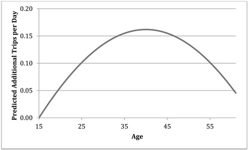
The direct-effect submodel on trip making produces results that are for the most part consistent with the cross-sectional models presented above. Women make more trips than men; Hispanics make more trips than Whites, who in turn make more trips than Blacks, Asians, and others. Education, being employed, household income, and access to autos are all positively associated with trip-making; and living in more densely populated areas is associated with more trips. With respect to our variables of interest, daily web use increases, rather than depresses, trips and young adults living with their parents tend to make fewer trips, all things equal. Age, controlling for other factors, has a small but meaningful influence on trip-making. As Figure 25 shows, the model suggests that trip-making increases until age 40, at which point it begins declining.
Figure 25: Estimated Independent Effect of Age on Trip-Making (age 15=0)
Independent of age, income effects, and auto ownership effects, one’s birth cohorts appears to have little direct influence trip-making, though there is an effect for two cohorts. Relative to those born before 1950, those born in the 1960s make more trips, while those born in the 1990s make fewer trips.
Figure 26: Combined Direct and Indirect Effects on Trip-Making of Birth Cohort
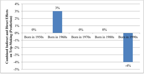
The combined indirect and direct effects of one’s birth cohort, however, are shown in Figure 26. These combined coefficients suggest that, while living in households that have more automobiles on average than did previous cohorts at the same stage in their lives, those born in the 1990s are making fewer trips on average that all previous cohorts. Again, as above, we urge caution in interpreting these results, as the short window (1990-2009) of our analysis does not allow for true comparisons with all previous cohorts. Including the survey years as dummy variables in the models should account for period effects (such as an economic downturn in 1990 and depressed trip-making after 9/11 in 2001) on trip-making, and indeed trip rates in both 2001 and 2009 are statistically significantly lower than in 1990.
| Sub-Model: Ratio of Cars to Adults | ||||
|---|---|---|---|---|
| Coefficient | Sig. | t-Statistic | p-value | |
| Individual Characteristics | ||||
| Race / Ethnicity (omitted category: Non-Hispanic White) | ||||
| Non-Hispanic Black | -0.122 |
*** |
-28.47 |
<0.001 |
| Non-Hispanic Asian (2009 Only) | -0.103 |
*** |
-17.27 |
<0.001 |
| Non-Hispanic Other | -0.040 |
*** |
-3.77 |
<0.001 |
| Hispanic | -0.064 |
*** |
-17.03 |
<0.001 |
| Household Characteristics | ||||
| Number of Adults in HH | -0.130 |
*** |
-99.54 |
<0.001 |
| Income (ln) | 0.145 |
*** |
125.88 |
<0.001 |
| Geographic Characteristics | ||||
| Population Density (ln) | -0.063 |
*** |
-102.55 |
<0.001 |
| Year (base:1990) | ||||
| Year: 2001 | 0.230 |
*** |
56.1 |
<0.001 |
| Year: 2009 | 0.242 |
*** |
60.94 |
<0.001 |
| Cohorts (base: Born before 1950) | ||||
| Born in 1950s | 0.023 |
*** |
7.35 |
<0.001 |
| Born in 1960s | 0.010 |
*** |
3.15 |
0.003 |
| Born in 1970s | -0.039 |
*** |
-11.04 |
<0.001 |
| Born in 1980s | 0.034 |
*** |
7.85 |
<0.001 |
| Born in 1990s | 0.118 |
*** |
20.76 |
<0.001 |
| Constant | -0.423 |
*** |
-31.4 |
<0.001 |
| Sub-Model: Income (ln) | ||||
|---|---|---|---|---|
| Coefficient | Sig. | t-Statistic | p-value | |
| Individual Characteristics | ||||
| Race / Ethnicity (omitted category: Non-Hispanic White) | ||||
| Non-Hispanic Black | -0.419 |
*** |
-61.34 |
<0.001 |
| Non-Hispanic Asian (2009 Only) | -0.140 |
*** |
-14.57 |
<0.001 |
| Non-Hispanic Other | -0.201 |
*** |
-19.49 |
<0.001 |
| Hispanic | -0.334 |
*** |
-54.93 |
<0.001 |
| Education (omitted category: No HS Diploma) | ||||
| For Youth: Highest Degree Achieved in Household | ||||
| High School Diploma | 0.368 |
*** |
40.12 |
<0.001 |
| Some College | 0.567 |
*** |
70.69 |
<0.001 |
| Bachelor's Degree | 1.045 |
*** |
110.59 |
<0.001 |
| Graduate Degree | 1.363 |
*** |
129.37 |
<0.001 |
| For Adults: Highest Degree Personally Achieved | ||||
| High School Diploma | 0.591 |
*** |
62.05 |
<0.001 |
| Some College | 0.903 |
*** |
96.08 |
<0.001 |
| Bachelor's Degree | 1.318 |
*** |
137.76 |
<0.001 |
| Graduate Degree | 1.597 |
*** |
164.04 |
<0.001 |
| Reports Working | 0.281 |
*** |
57.07 |
<0.001 |
| Household Characteristics | ||||
| Number of Adults in HH | 0.125 |
*** |
58.7 |
<0.001 |
| Youth, Lives with Parents | -0.192 |
*** |
-2.78 |
0.005 |
| Year (base: 1990) | ||||
| Year: 2001 | -0.110 |
*** |
-16.24 |
<0.001 |
| Year: 2009 | -0.175 |
*** |
-25.33 |
<0.001 |
| Cohorts (base: Born before 1950) | ||||
| Born in 1950s | 0.009 |
* |
1.75 |
0.081 |
| Born in 1960s | 0.028 |
*** |
5.25 |
<0.001 |
| Born in 1970s | -0.055 |
*** |
-8.91 |
<0.001 |
| Born in 1980s | -0.045 |
*** |
-4.75 |
<0.001 |
| Born in 1990s | 0.350 |
*** |
28.05 |
<0.001 |
| Constant | 9.811 |
*** |
847.77 |
<0.001 |
| Sub-Model: Number of Activities (ln) | ||||
|---|---|---|---|---|
| Coefficient | Sig. | t-Statistic | p-value | |
| Individual Characteristics | ||||
| Female | 0.068 |
*** |
24.28 |
<0.001 |
| Age | 0.006 |
*** |
3.79 |
<0.001 |
| Age Squared | <0.001 |
*** |
-4.73 |
<0.001 |
| Race / Ethnicity (omitted category: Non-Hispanic White) | ||||
| Non-Hispanic Black | -0.020 |
*** |
-6.55 |
0.001 |
| Non-Hispanic Asian (2009 Only) | -0.111 |
*** |
-13.16 |
<0.001 |
| Non-Hispanic Other | -0.046 |
*** |
-5.95 |
<0.001 |
| Hispanic | 0.025 |
*** |
2.87 |
<0.001 |
| Education (omitted category: No HS Diploma) | ||||
| For Youth: Highest Degree Achieved in Household | ||||
| High School Diploma | 0.072 |
*** |
5.26 |
<0.001 |
| Some College | 0.134 |
*** |
10.47 |
<0.001 |
| Bachelor's Degree | 0.139 |
*** |
10.48 |
<0.001 |
| Graduate Degree | 0.165 |
*** |
11.25 |
<0.001 |
| For Adults: Highest Degree Personally Achieved | ||||
| High School Diploma | 0.030 |
* |
3.14 |
0.002 |
| Some College | 0.099 |
*** |
10.67 |
<0.001 |
| Bachelor's Degree | 0.158 |
*** |
16.54 |
<0.001 |
| Graduate Degree | 0.209 |
*** |
21.30 |
<0.001 |
| Reports Working | 0.118 |
*** |
34.21 |
<0.001 |
| Uses Web Daily | 0.064 |
*** |
19.25 |
<0.001 |
| Household Characteristics | ||||
| Income (ln) | 0.034 |
*** |
17.47 |
<0.001 |
| Number of Adults in HH | -0.037 |
*** |
-19.62 |
<0.001 |
| Youth, Lives with Parents | -0.054 |
*** |
-6.30 |
<0.001 |
| Ratio of Cars to Adults in HH | 0.057 |
*** |
18.80 |
<0.001 |
| Geographic Characteristics | ||||
| Population Density (ln) | 0.017 |
*** |
19.89 |
<0.001 |
| Year (base: 1990) | ||||
| Year: 2001 (base: 1990) | -0.037 |
*** |
-4.97 |
<0.001 |
| Year: 2009 (base: 1990) | -0.107 |
*** |
-10.82 |
<0.001 |
| Cohorts (base: Born before 1950) | ||||
| Born in 1950s | 0.005 | 0.74 | 0.458 | |
| Born in 1960s | 0.032 |
*** |
3.18 |
0.001 |
| Born in 1970s | -0.011 | -0.78 | 0.437 | |
| Born in 1980s | -0.024 | -1.29 | 0.198 | |
| Born in 1990s | -0.058 |
** |
-2.49 |
0.013 |
| Constant | 0.424 |
*** |
23.84 |
<0.001 |
| Variance | ||||
| Var (Ratio of Cars to Adults) | 0.213 | |||
| Var (Income (ln)) | 0.560 | |||
| Var (Number of Activities (ln)) | 0.414 | |||
| N | 265,543 | |||
| R2 (Overall) | 0.409 | |||
| Key: Statistically Significant | ||||
G. Conclusion: Youth, Activities, and Trips
The demand for travel is derived. That is, people travel in order to access opportunities to do, acquire, or sell. With the exceptions of long walks on the beach or cruising the boulevard on a Saturday night, people—as members of households or employees of firms—travel in order to do other things. Thus trips, as opposed to traveling, act as a proxy for activity participation; the more trips one completes, the more activities in which s/he participates. Up to a point, therefore, more trips mean more activities and access to a higher quality of life.22 Likewise, more time and money spent traveling to a fewer number of destinations means fewer trips and lower levels of personal access, in spite of high levels of mobility. Accordingly, this analysis focuses on trip-making and trip purpose in order to examine the access, or utility that people derive from their trips.
Drawing on the literature, we hypothesize that adults make more trips than youth, and that higher incomes and greater private vehicle access are associated with higher levels of trip-making and, hence, activity participation—and indeed we find these to be the case. In general, trip-making increases year to year as people age from the early teens through late middle-age, and then it declines gradually thereafter. Trip-making is highly correlated with economic activity, as we observe that trips per person increased between 1990 and 2001, but declined between 2001 and the recession of 2009. Unemployment in 2009 was substantially higher among youth than adults, and the drop in trip-making between 2001 and 2009 was greater for youth than for adults. And at a more micro level, our analysis shows that both income and employment are associated with greater trip-making.
To examine the independent effects of income, auto access, employment, information and communications technologies use, and driver’s licensing regimes on trip-making of both youth and adults, we constructed a set of structural equation models (SEMs). We find in these models that income is a powerful predictor of trip-making among adults, and its importance in predicting youth trips increased substantially between 1990 and 2009 and is now on par with that of adults. The most important effect of income is increased automobile access, which in turn encourages more trips. While income and working are strongly associated with increased trip-making among both adults and, increasingly, youth, time spent commuting to and from work – because it reflects the opportunity cost of time – tends to depress trip-making.
| Youth (15–26) 1990 |
Youth (15–26) 2001 |
Youth (15–26) 2009 |
Adult (27–61) 1990 |
Adult (27–61) 2001 |
Adult (27–61) 2009 |
|
|---|---|---|---|---|---|---|
| Worker Status | + |
+ |
+ |
+ |
+ |
+ |
| Young Adult Living at Home | (Not included in the model) | |||||
| Technology (Web Use) | n/a | 0 |
0 |
n/a | + |
+ |
| License Stringency | - |
+ |
- |
- |
+ |
- |
While the effects of the economy, income, auto access, and working are all positively associated with trip-making among both adults and youth, internet access appears to have no effect on youth trip-making, and may actually be associated with a slight increase in adult trip-making in 2009. Likewise, and remarkably, increasingly strict licensing regimes for teens appear to have little, if any, effect on youth trip-making. Finally, we note in these models that the independent effects of race/ethnicity on trip-making appear to be waning over time, especially among youth.
We also constructed a quasi-cohort model of auto access (measured as autos per adult), income, and activities (measured as daily trips). In the submodel predicting the ratio of cars to household adults, respondents in 2001 and 2009 were substantially more likely to have access to autos than respondents in 1990, ceteris paribus, and those born in the 1990s in particular have remarkably high automobile access. Similarly, today’s teens are living in households that have considerably higher incomes than was the case for prior generations, after controlling for the period effect of the current economic recession. Taken together, though, the negative direct effect of being born in the 1990s on trip-making overwhelms the positive effect of income and auto ownership, and those born in the 1990s are estimated to make roughly four percent fewer trips than previous cohorts did at the same age in their lives, all else equal.
22While a few more trips at the margin are assumed to be a positive measure of accessibility, a very large number of trips in a given day is obviously excessive and burdensome. Accordingly, as we explained above, we have log-transformed our trips measure to mute the effect of large numbers of trips in our analysis.