
Chapter V. Personal Miles Traveled (PMT)
A. Introduction
The NPTS and NHTS offer a wide variety of measures of travel behavior to estimate daily mobility. Personal miles traveled (PMT) is a standard measure of mobility that combines both the number and length of trips. While generally mode- and area-neutral, PMT do tend to be higher among drivers and among those who live in suburbs. In this chapter, we begin by describing our methodology for analyzing PMT, focusing on aspects of the methodology unique to this analysis. We then present descriptive data for our outcome measure (PMT) and for a few of our variables of interest. Finally, the chapter concludes with our statistical models and overall findings.
B. Methodology
Our cross-sectional models predict personal miles traveled (PMT) according to the following function:
PMT = f(I, H, N, R, u)
To determine individual PMT values we summed the distance of all trips by all modes on the survey day.14 Individual characteristics (I) include a set of personal characteristics shown to influence travel behavior such as sex, age, race/ethnicity, education, employment status, driver. In this category, we also include daily use of the web, a variable that has not been widely tested relative to PMT. To each individual record we also attach household characteristics (H), including household income (ln), the number of adults and children in the household, and the number of autos per adult in the household. For youth, we add to these standard determinants a variable identifying whether young adults live with their parents. Residential location characteristics (N) include population density of the respondent’s census tract and whether the individual lives in a large metropolitan area. Finally, we include a variable (R) identifying the stringency of the state driver’s licensing regulations.
As we described previously, for this analysis, we analyze three age groups: teens (15–18), young adults (19–26), and adults (27–61). The inclusion of the teen age group captures the transformational period for travel behavior when most teens obtain driver’s licenses. These age groupings also correspond to a period when teens are likely to move out of their parents’ homes. In 2009, approximately 88 percent of respondents aged 15 to 18 live with their parents, but at age 19 the figure falls to 74 percent and declines steadily thereafter with age.
We specified a large variety of models to predict PMT. In our analysis, we sought to compare regression coefficients for specific variables across these models and survey years. As a result, we needed to apply the same overall model specification to each year and age group. The optimal model would explain the variation in PMT equally well in each of the three model years and for each of the three age groups. This presents obvious analytical challenges, particularly because any given model is likely to fit one year and age group better than the other years. Moreover, any changes made to a single model required making changes to each of the eight additional models.
Initially we tried to model license regulations and driver status in the same PMT model. We found that license regulations were not statistically significantly related to PMT, but such models had serious endogeneity issues, especially for teens. To address these issues we ran two separate models—one with driver status (Table 17) as an independent variable and the other with information on licensing regulations (Table 18). Contrary to our expectations, the stringency of license regulations does not appear to influence PMT for teens. As a result, we consider the model with driver status our primary model.
In a separate model, we test to see whether there are cohort effects. The quasi-cohort model is a standard linear regression model of PMT, and it closely resembles the cross-sectional models. To test whether individuals in more recent age cohorts travel differently from prior cohorts, controlling for other factors, we introduce a series of decade-of-birth (cohort) variables. We include a year variable to account for period effects (such as the economic boom of the 1990s and the economic collapse of the late 2000s) not captured by any of the other independent variables.
C. Descriptive Statistics
In this section, we describe our data, starting with data on PMT by age group and year. We then highlight some of the data related to other variables of interest—driver status and graduated driver’s licensing, employment, living with parents, and web use.
PMT: Figure 12 presents mean PMT levels for each of the age categories over the three research periods. Between 1990 and 2001, PMT increased for individuals in all three age categories before declining again in 2009, undoubtedly related to the recession. In general, PMT is positively related to age, and PMT typically increases dramatically as teens transition into young adulthood. However, in 1990, young adults traveled more miles than both teens (expected) and adults (not expected). This pattern changed with the 2001 and 2009 surveys wherein teens travel less than young and older adults, and the primary increase in PMT occurs by the time respondents are young adults.
Figure 12: Personal Miles Traveled by Age Group and Year (1990, 2001, and 2009)
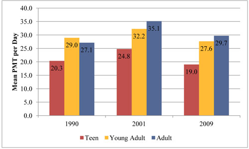
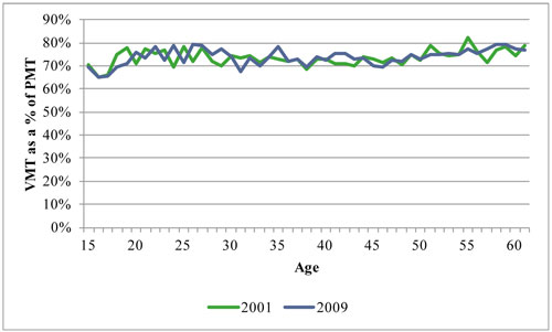
Table 11 and Figure 13 show vehicle miles traveled (VMT) as a percentage of PMT by age. As expected, for both years, the percentage of VMT to PMT is lowest for young teens, under 70 percent. However, the percentage of VMT to PMT is slightly higher for young adults than adults. Finally, between 2001 and 2009, the percentage of VMT to PMT increased slightly for both young adults and adults; however, it declined for teens.
| 2001 | 2009 | |
|---|---|---|
| Teen (15-18) | 69.6% | 67.7% |
| Young Adult (19-26) | 74.5% | 75.1% |
| Adult (27-61) | 73.4% | 74.1% |
Figure 13: Vehicle Miles Traveled as Percentage of PMT by Age (2001 and 2009)
Driver Status: We hypothesize that being a driver (“driver status”) will influence PMT. Individuals who can drive will be more likely to travel by automobile than other, slower modes of transportation and, therefore, will likely travel more miles than non-drivers. Having a driver’s license (a proxy for driver status) is positively associated with the number of person trips and negatively associated with transit and non-motorized travel (Kitamura et al., 1997).
Table 12 presents PMT by age group and driver status for each survey year. There are several noteworthy aspects of the table. First, as predicted, drivers have substantially higher average PMT than non-drivers do. However, the difference in PMT for drivers and non-drivers is greater for adults than for teens. Figure 12 also depicts an increase in PMT between 1990 and 2001, and a subsequent decrease in 2009 to figures similar to or lower than 1990 values.
| 1990 | 2001 | 2009 | |
|---|---|---|---|
| Teen (15–18) | |||
| Non-Driver | 15.7 | 18.5 | 14.3 |
| Driver | 25.9 | 30.0 | 22.8 |
| % Difference (Driver/Non-Driver) | 65.0% | 62.2% | 59.4 |
| Young Adult (19–26) | |||
| Non-Driver | 14.9 | 13.6 | 13.0 |
| Driver | 30.6 | 34.8 | 29.9 |
| % Difference (Driver/Non-Driver) | 105.4% | 155.9% | 130.0% |
| Adult (27–61) | |||
| Non-Driver | 11.9 | 14.5 | 10.1 |
| Driver | 28.1 | 36.3 | 31.1 |
| % Difference (Driver/Non-Driver) | 136.1% | 150.3% | 207.9% |
Table 13 presents PMT by age group and stringency of the licensing regime. We can see that PMT is significantly lower for respondents in states with stricter license regimes in every year. Surprisingly, this result holds for all ages in most years, suggesting some underlying effect in those states on both licensing regimes and PMT, rather than an independent effect of licensing on PMT.
| 1990 | 2001 | 2009 | |
|---|---|---|---|
| Teen (15–18) | |||
| License Stringency: Lowest | 20.8 | 27.5 | |
| License Stringency: Low | 16.9 | 24.5 | 25.3 |
| License Stringency: Med | 24.8 | 19.3 | |
| License Stringency: High | 21.8 | 18.5 | |
| Average for all Teens | 20.3 | 24.8 | 19.0 |
| Young Adult (19–26) | |||
| License Stringency: Lowest | 29.3 | 34.4 | |
| License Stringency: Low | 28.1 | 34.5 | 31.1 |
| License Stringency: Med | 29.7 | 27.4 | |
| License Stringency: High | 33.0 | 27.5 | |
| Average for all Young Adults | 29.0 | 32.2 | 27.6 |
| Adult (26-61) | |||
| License Stringency: Lowest | 27.5 | 36.1 | |
| License Stringency: Low | 25.9 | 35.4 | 32.7 |
| License Stringency: Med | 34.2 | 30.2 | |
| License Stringency: High | 36.7 | 29.3 | |
| Average for all Adults | 27.1 | 35.1 | 29.7 |
Employment: Being employed is positively related to PMT as traveling to, from, and during work contribute significantly to total trips and miles. Data from the 2009 NHTS show that commute and work-related travel comprise 19 percent of all person trips and 25 percent of all PMT (Santos et al., 2011).
Table 14 presents PMT figures by employment status in 2009. The figures for 2001 and 1990 are broadly similar and can be found in the Appendix (Table 49). We see that employed respondents of any age have higher average PMT than people who are unemployed. Adults and young adults travel further on average if they are employed full-time. Teenagers have higher average PMT if they are employed part-time than if they are employed full-time or not employed at all. This finding reflects the fact that teenagers with part-time employment are likely still in school and, therefore, might need to travel to more destinations.
| Teen (15–18) | Young Adult (19–26) | Adult (27–61) | |
|---|---|---|---|
| Not Worker | 17.3 | 21.3 | 20.6 |
| Work Full Time | 20.7 | 31.7 | 33.0 |
| Work Part Time | 24.0 | 28.0 | 26.2 |
| Average | 19.0 | 27.6 | 29.7 |
Sex Differences: There is a well-established literature on the relationship between gender and travel. With respect to PMT, for example, Rosenbloom (2006) analyzes NHTS data and finds that women travel less distance than men do—on average 63 percent less in 2001. Gender differences in travel differ by age and appear to widen over time; Rosenbloom (2006) reports that women aged 16 to 24 travel 82 percent as far on average as men of the same age. Sex differences persist when controlling for other factors such as age, number of children, income, and employment (Giuliano 2003).
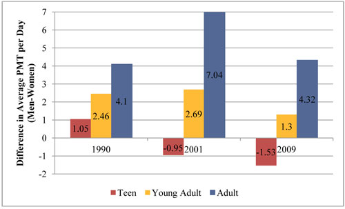
Figure 14 presents the average sex differences in PMT by age group and year between 1990 and 2009. Consistent with most previous studies, we find that men do indeed travel farther than women, and this gap tends to widen through adulthood. For teens in 2001 and 2009, however, we find that women actually travel farther on average than men. Whether this is a cohort or life-cycle effect remains to be seen; given that this trend of greater PMT by teen girls/women than teen boys/men appears to be growing over time suggests that this may be a cohort effect that could persist.
Figure 14: Sex Differences in PMT by Age and Year (1990, 2001, and 2009)
Web Use: As Table 15 shows, people who use the internet daily have higher average PMT than people who use the web less frequently, and the gap is larger for older age groups than for younger age groups. This finding suggests that web use is not a substitute for travel, as many individuals have hoped. However, daily web use is correlated with income, which is also a strong predictor of PMT. The apparent relationship between web use and PMT may thus actually reflect the effect of income on both web use and travel.
| Teen (15–18) | Young Adult (19–26) | Adult (27–61) | |
|---|---|---|---|
| Does not use the web daily | 16.3 | 25.5 | 24.5 |
| Uses the web daily | 18.6 | 28.2 | 32.0 |
| % Difference (Uses Daily/Not Use Daily) | 87.4% | 90.5% | 76.6% |
Living With Parents: The late teen and early 20s years are periods of considerable transition for most people. Some transition into college, and others into the workforce; some move out to form their own households, some stay at home, and some “boomerang” back home after living independently for a time. The effects of these various transitions are complex and difficult to characterize. Table 16 shows that young people living with their parents have higher average PMT than young people who do not live with their parents across all three survey years; however, this gap is decreasing over time.
| 1990 | 2001 | 2009 | |
|---|---|---|---|
| Does not Live with Parents | 21.1 | 24.7 | 28.9 |
| Lives With Parents | 27.3 | 27.9 | 31.3 |
| % Difference (Does not Live with Parents/Lives with Parents) |
77.0% | 88.4% | 92.1% |
D. Cross-Sectional Models and Model Results
Table 17 and Table 18 present our multivariate statistical analyses of PMT that attempt to simultaneously account for the independent effects of the factors discussed above, as well as other control variable factors known to influence travel behavior. We first examine the results presented in Table 17, which show the models that include a “driver” variable, but no licensing regime data. In the conclusion, we discuss the second set of models presented in Table 18, which exclude the driver status variable and include graduated driver’s license regulations data.
The most consistent and substantial effects on PMT across age groups and survey years are whether the respondent is employed and whether s/he drives.15 In all of the models, employment is consistently and positively related to PMT for all age groups in all years. Moreover, the magnitude of the effect appears to be increasing for all age groups over time. Second, driver status has a positive effect on PMT for all age groups, and the effect has increased in magnitude for all groups since 1990. The magnitude of the effect is smaller for teens and young adults than for adults, but this youth/adult gap has diminished over time.
The coefficients for household income in our models can be interpreted as elasticities. For example, the coefficient of +0.14 for adults in 2009 signifies that as household income doubles, personal miles traveled increases by 14 percent. Even after controlling for a wide variety of other factors, household income is positively associated with PMT for adults; however, household income is not significantly related to personal travel for teens.16
Income is powerfully and positively associated with travel in the literature, so why do our models show that income is unrelated to the travel behavior of teens? Income is highly correlated with both being employed and owning an automobile. Similarly, being employed increases the probability that one will own a car and, conversely, access to autos increases the likelihood of being employed (Baum, 2009; Gurley and Bruce, 2005; Ong, 2002). Because we include employment and driver status variables, the relatively muted observed effects of income on PMT are not surprising. Not surprisingly, people living in households with higher levels of auto access tend to travel more. Individuals living in households with more automobiles per adult tend to have higher PMT than individuals with fewer automobiles per adult. In contrast to the household income effect, the effect of auto access is larger for teens and young adults than it is for adults.17 This suggests that older adults are more likely to have “first call” on household autos, such that increasing the autos-to-adults ratio has a disproportionate effect on youth auto access, driving, and PMT.
Consistent with the descriptive statistics presented above, we find no evidence that daily web use is a substitute for personal travel, among teens, young adults, or adults. With just one exception, the relationship between daily web use and PMT is not statistically significant in the models for all age groups and years. The one exception we observe is that the relationship between web use and PMT is significant and positive for adults in 2009, indicating that, all else equal, PMT is higher for people who use the internet daily than for people who do not use the internet daily. In the models focusing on the stringency of licensing regimes, we again find web use is not a substitute to travel for all three age groups in 2009.
Household structure affects travel patterns differently by age group. In 2001 and 2009, for each additional adult in the household, teens report an increase in PMT. Conversely, for adults the addition of another adult in the household had a negative relationship with PMT in 1990, suggesting that more adults were dividing a relatively fixed amount of household-serving travel. The addition of another child in the household increases personal travel for adults, perhaps due to increased chauffeuring and other household-serving travel responsibilities associated with children. Conversely, and perhaps logically, additional children are associated with decreased personal travel for teens and young adults in 1990, but this observed effect is not statistically significant in the two more recent surveys. Finally, and contrary to our expectations, we find that living with one’s parents has no significant effect, either positive or negative, on PMT among young adults.
The geographic variables analyzed are associated with personal travel in much the same way for all age groups. We use a log-transformed value to represent density so the coefficient can be interpreted as an elasticity. The coefficient of -0.17 for youth in 2001 indicates that doubling the population density is associated with a 17 percent decrease in PMT. Without exception, population density is negatively related to PMT. The hypothesized effect here is two-fold: first, higher densities place trip origins and destinations closer together, which shorten the distances needed to travel to desired destinations; second, higher densities are associated with more traffic congestion and limited and expensive parking, both of which discourage automobile use. In contrast to the observed effects of population density, the dummy (1 = yes, 0 = no) variable for individuals in a metropolitan area with over 3 million people does not generally contribute to our understanding of PMT.
There are some surprising results with respect to a few of the other control variables in our models. In most cases, we find little evidence of a relationship between sex and PMT, after controlling for a wide array of other factors. There are two exceptions, which together suggest that sex influences travel differently depending on individuals’ stage of life. In 2009, female teens had higher average PMT than otherwise similar male teens. Among adults, however, being female tends to be negatively associated with PMT, although only statistically significant in 2001. Whether this is a life-cycle effect—meaning that we can expect that women will typically travel more than men in their teens and less than men at retirement—or a cohort effect—meaning that the era of greater male PMT is waning, and an era of greater PMT by women is waxing—remains to be seen, though the fragmentary evidence presented here suggests that this may be a cohort effect.
The observed effects of race/ethnicity on PMT in 2009 point to possible changes to patterns of race/ethnicity and travel observed historically (Doyle and Taylor, 2000; Taylor and Ong, 1995). The race/ethnicity variables are dummy (1 = yes, 0 = no) variables and should be interpreted as a group. The joint effect of the race/ethnicity variables on PMT were statistically significant for adults in 1990 and 2009 and for young adults in 2001, but were never significantly related to PMT for teens.
The results suggest that the relationship between race/ethnicity and PMT for adults has changed dramatically between 1990 and 2009. In 1990, and consistent with the literature, both Hispanics and Blacks had lower PMT (all else being equal) compared with Non-Hispanic Whites (who serve as the omitted, or base, case in the models). This suggests that, even after controlling for the lower average household incomes and lower levels of auto access in Hispanic and Black households, personal travel was still lower compared with non-Hispanic Whites. In 2009, however, we observe precisely the opposite effect: after controlling for a wide variety of factors thought to influence personal travel, Hispanic and Black respondents in 2009 had higher PMT than comparable Non-Hispanic Whites.18
Given our descriptive statistics show that PMT increases with age into late middle-age, our model results for age, particularly for teens, are also counterintuitive. According to the model, older teens travel less far than younger teens, everything else held equal. This surprising finding may be because age is highly correlated with employment, web use, and driver status, which are all included in the model.
Finally, we present the results of the license stringency model in Table 18. We do not find the strictness of state licensing regulations to be statistically significantly related to PMT for teens in 1990, 2001, or 2009. To be sure that we were not somehow missing the effect of regulations on teen travel, we examined each age separately. Doing so uncovered a statistically significant relationship between licensing regulations and PMT for 16 year olds in 2001 only.19 This single exception notwithstanding, stricter licensing regimes—at least as we have measured them here—do not appear to substantially hinder the personal mobility of American teens.
If driving and auto access are so strongly and positively associated with personal travel, how can making it tougher for teens to get licenses and drive not affect their PMT? One answer may lie with our data. While the particulars of the licensing restrictions vary substantially from state to state, most have for the most part been moving toward tougher licensing regulations in concert with one another. But for licensing restrictions to explain any of the variation in PMT in our models, the state licensing restrictions themselves must vary sufficiently from one another. But in 1990 and 2009 there is very little variation in the license ranking across states. In 1990, most states (42) had the lowest stringency regulations (Poor); by 2009, a majority of states (30) had high stringency regulations (Good). The year 2001 represents a transitional period in which there was substantial variation in licensing restrictions across the states.
Moreover, just because a law is on the books does not guarantee compliance. For example, in a study of young drivers in North Carolina, Goodwin and Fost (2004) find that although knowledge of license restrictions is widespread, teenagers frequently violate license restrictions, particularly passenger restrictions, and that enforcement is typically a low priority for police officers. It is possible that young drivers are not dissuaded from getting a drivers license and/or are not reducing the number of miles they drive because the ostensibly tight restrictions are simply poorly enforced. Finally, it is possible that the regulations have little effect on PMT in metropolitan areas where individuals may be able to travel relatively more readily by other modes such as carpool and public transit. If this is the case, we might expect driver’s licensing regulations to influence mode choice—the subject of Chapters 8 and 9 of this report.
Finally, and contrary to expectations, the licensing variable is significantly related to the PMT of young adults and adults in some survey years. This suggests that the licensing variable may not only capture the strength of licensing, but also some other unknown statewide effect that influences the travel behavior of people beyond the teenage years.
| Teen 1990 |
Teen 2001 |
Teen 2009 |
Young Adult 1990 |
Young Adult 2001 |
Young Adult 2009 |
Adult 1990 |
Adult 2001 |
Adult 2009 |
|
|---|---|---|---|---|---|---|---|---|---|
| Individual Characteristics | |||||||||
| Age | -0.39*** |
-0.05 | -0.58*** |
-0.02 | -0.01 | 0.03 | -0.01*** |
-0.01*** |
0.00 |
| Female | -0.06 | -0.08 | 0.21* |
-0.02 | 0.01 | 0.13 | 0.03 | -0.15*** |
0.06 |
| NH White | omitted | omitted | omitted | omitted | omitted | omitted | omitted | omitted | omitted |
| NH Black | -0.02 | 0.08 | 0.17 | -0.49* |
0.13 | 0.37** |
-0.20* |
-0.01 | -0.20** |
| NH Asian | no data | 0.06 | -0.32 | no data | -0.01 | 0.16 | no data | -0.17 | 0.08 |
| Hispanic | -0.11 | -0.26 | 0.21 | -0.39 | -0.18 | 0.26* |
-0.19* |
-0.15 | 0.20*** |
| NH Other | -0.07 | -0.18 | -0.02 | -0.37 | -0.03 | 0.31 | 0.00* |
0.19*** |
-0.28* |
| Employed | 0.60*** |
0.63*** |
0.85*** |
-0.97*** |
0.98*** |
1.20** |
0.95*** |
0.94*** |
1.06*** |
| Web Use Daily | no data | 0.09 | 0.19 | no data | 0.03 | 0.16 | no data | -0.01 | 0.19*** |
| Driver | 0.35* |
0.60*** |
0.82*** |
0.40* | 1.54*** |
1.17** |
1.08*** |
1.22*** |
1.67*** |
| Less than High School | omitted | omitted | omitted | omitted | omitted | omitted | omitted | omitted | omitted |
| High School Graduate | -0.37 | 0.53 | 0.74 | 0.18 | 0.24 | 0.22 | 0.19* |
0.21** |
0.28** |
| Some College | -0.31 | 0.61 | 0.64 | 0.15 | 0.43 | 0.29 | 0.53*** |
0.43*** |
0.37*** |
| College Graduate | -0.66* |
0.76* |
0.84* |
0.22 | 0.66** |
0.42 | 0.49*** |
0.54*** |
0.49*** |
| Grad or Prof. Degree | -0.35 | 0.76* |
0.92* |
0.50 |
0.68** |
0.47 | 0.61*** |
0.55*** |
0.47*** |
| Young Adult Lives with Parents | -0.24 | -0.03 | -0.02 | ||||||
| Household Characteristics | |||||||||
| Household Income (ln) | 0.08 | -0.05 | -0.01 | 0.11 | -0.05 | -0.01 | 0.12*** |
0.18*** |
0.14*** |
| Number of Adults | -0.09 | 0.19*** |
0.16** |
-0.01 | 0.04 | -0.09 | -0.11** |
-0.01 | -0.02 |
| Number of Children | -0.13* |
-0.09 | -0.10 | -0.11 |
0.01 | 0.03 | 0.02 | 0.08*** |
0.11*** |
| Autos Per Adult | 0.59*** |
0.13 | 0.24** |
0.47*** |
0.38*** |
0.46** |
0.22*** |
0.18*** |
0.19*** |
| Geographic Characteristics | |||||||||
| Population Density (ln) | 0.04 | -0.17*** |
-0.10** |
-0.06 | -0.06** |
-0.08* |
-0.09*** |
-0.08*** |
-0.05*** |
| MSA > 3 million | 0.03 | -0.19 | 0.03 | 0.08 | -0.21** |
0.18 | 0.08 | 0.04 | -0.02 |
| Constant | 7.39*** |
1.84 | 9.31*** |
-0.01 | 0.33 | -1.09 | -0.76* |
-1.68*** |
-2.64*** |
| Model N | 1252 | 5514 | 9464 | 3185 | 7565 | 9003 | 13167 | 56269 | 104289 |
| Adjusted R2 | 0.09 | 0.09 | 0.11 | 0.10 | 0.12 | 0.10 | 0.11 | 0.09 | 0.12 |
| KEY: |
|---|
| Statistically Significant |
| Statistically Significant Over Time (across all the years for which data were available) |
| Teen 1990 |
Teen 2001 |
Teen 2009 |
Young Adult 1990 |
Young Adult 2001 |
Young Adult 2009 |
Adult 1990 |
Adult 2001 |
Adult 2009 |
|
|---|---|---|---|---|---|---|---|---|---|
| Individual Characteristics | |||||||||
| Age | -0.10 | 0.06 | -0.45*** |
-0.02 | 0.00 | 0.04 | -0.01*** |
-0.01** |
0.00* |
| Female | -0.05 | -0.09 | 0.21* |
-0.02 | -0.01 | 0.15 | 0.01 | -0.16*** |
0.04 |
| NH White | omitted | omitted | omitted | omitted | omitted | omitted | omitted | omitted | omitted |
| NH Black | 0.00 | 0.05 | 0.11 | -0.52** |
0.09 | 0.38** |
-0.24** |
-0.02 | 0.18** |
| NH Asian | no data | -0.06 | -0.45 | no data | -0.10 | 0.18 | no data | -0.19* |
0.04 |
| Hispanic | -0.23 | -0.26 | 0.13 | -0.38 | -0.33 | 0.30* |
-0.28** |
-0.16 | 0.19*** |
| NH Other | -0.14 | -0.20 | -0.13 | -0.38 | -0.13 | 0.32 | -0.45** |
0.20*** |
-0.30* |
| Employed | 0.70*** |
0.69*** |
0.99*** |
0.99*** |
1.12*** |
1.29*** |
1.00*** |
1.04*** |
1.23*** |
| Web Use Daily | no data | 0.07 | 0.26* |
no data | 0.07 | 0.28* |
no data | 0.00 | 0.26*** |
| Less than High School | omitted | omitted | omitted | omitted | omitted | omitted | omitted | omitted | omitted |
| High School Graduate | -0.14 | 0.51 | 0.68 | 0.21 | 0.33 | 0.36 | 0.27** |
0.32*** |
0.45*** |
| Some College | -0.11 | 0.64 | 0.59 | 0.17 | 0.59** |
0.50 | 0.63*** |
0.56*** |
0.60*** |
| College Graduate | -0.38 | 0.80* |
0.80* |
0.24 | 0.86*** |
0.64 | 0.60*** |
0.68*** |
0.72*** |
| Grad or Prof. Degree | -0.15 | 0.83* |
0.92** |
0.53* |
0.86*** |
0.69 | 0.71*** |
0.69*** |
0.69*** |
| Young Adult Lives with Parents | omitted | omitted | omitted | -0.27* |
-0.14 | -0.08*** |
omitted | omitted | omitted |
| Household Characteristics | |||||||||
| Household Income (ln) | 0.10 | -0.01 | 0.05 | 0.11 | -0.03 | 0.00** |
0.15*** |
0.23*** |
0.18*** |
| Number of Adults | -0.08 | 0.18** |
0.16** |
-0.01 | 0.02 | -0.08*** |
-0.10** |
-0.03 | -0.02 |
| Number of Children | -0.17** |
-0.11* |
-0.12* |
-0.12* |
0.00 | 0.02 | 0.02 | 0.09*** |
0.13*** |
| Autos Per Adult | 0.66*** |
0.25* |
0.31*** |
0.55*** |
0.72*** |
0.74*** |
0.33*** |
0.27*** |
0.35*** |
| State Licensing Regulations | |||||||||
| Stringency: Lowest | omitted | omitted | omitted | omitted | omitted | omitted | omitted | ||
| Stringency: Low | -0.30 | 0.11 | 0.15 | -0.04 | omitted | -0.15** |
0.11* |
omitted | |
| Stringency: Medium | 0.22 | 0.48 | -0.04 | -0.14*** |
0.06 | -0.12 | |||
| Stringency: High | -0.08 | 0.44 | 0.30* |
-0.14*** |
0.16*** |
-0.12 | |||
| Geographic Characteristics | |||||||||
| Population Density (ln) | 0.06 | -0.18*** |
-0.09** |
-0.07 | -0.09*** |
-0.09** |
-0.10*** |
-0.10*** |
-0.06*** |
| MSA > 3 million | 0.04 | -0.20 | -0.08 | 0.04 | -0.28*** |
0.16 | 0.10 | 0.03 | -0.01 |
| Constant | 2.17 | -0.24 | 6.59*** |
0.23 | 0.82 | -0.86*** |
-0.24 | -1.36*** |
-1.94*** |
| Model N | 1324 | 5460 | 9514 | 3188 | 7499 | 9013 | 13176 | 55645 | 104294 |
| Adjusted R2 | 0.07 | 0.08 | 0.09 | 0.10 | 0.09 | 0.09 | 0.10 | 0.07 | 0.10 |
| KEY: |
|---|
| Statistically Significant |
| Statistically Significant Over Time (across all the years for which data were available) |
E. Quasi-Cohort Model Results
A central focus of this research is to examine whether the underlying factors influencing travel are changing over time – whether the next generation, or cohort, of American adults will travel differently than current or previous generations. The preceding analysis has been cross-sectional; that is, we have examined the constellation of factors that explain PMT in a given year for a given category of traveler and have reflected on how these appear to differ from year to year. To investigate this question via another method, we constructed models that consider the independent effects of cohorts of travelers by birth decade. Table 19 and Figure 15 show the results of this age cohort model. Many of the control variables operate as they did in the cross-sectional models above. One exception are the race/ethnicity variables; these showed mixed effects (positive, negative, statistically significant, and not) on PMT in the cross–sectional models, but in this cohort model we see some apparently counter-intuitive and statistically significant results. While non-Hispanic Whites tend to travel more and farther than non-Hispanic Blacks or Hispanics, income differences between these groups apparently explain much of the observed travel differences. Controlling for income, and a host of other factors, we see that being Black or Hispanic is associated more travel between 1990 and 2009. This is likely due to significant growth in auto access and use among Blacks and Hispanics during the 1990s and 2000s relative to non-Hispanic Whites (Pisarski 2006).
The year variable accounts for period effects (such as the economic boom of the 1990s and the economic collapse of the late 2000s) not captured by any of the other independent variables (for example, by income or employment status). Neither of these variables—for 2001 and 2009—are significantly different from 1990 (the base year), which suggests that period effects have been accounted for by the individual-level effects associated with these periods (e.g. employment status).
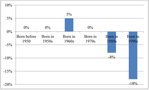
The model suggests that being born in a more recent decade – the 1980s and, in particular, the 1990s – is associated with lower PMT than those born in earlier decades, after controlling for a wide variety of other factors known to influence travel. One should keep in mind that those born in the 1980s and 1990s were still relatively young in the most recent data year, so these findings concern only the travel of teens and young adults. Specifically, the 1980s birth cohort compares 15 to 21 year-olds to similarly aged-cohorts born in the 1970s and 1990s, and 20 to 29 year-olds to similarly aged cohorts born in the 1960s and 1970s. The 1990s birth cohort compares only the travel of 15 to 19 year olds in 2009 to the 2001 travel of similarly aged people born in the 1980s and the 1990 travel of similarly aged people born in the 1970s. We present the independent effect of birth decade on PMT graphically in Figure 15. This figure suggests a strong and almost linear negative trend in the relationship between birth decade in the 1960s, 1970s, 1980s, and 1990s and PMT – again, after controlling for the other factors known to influence travel. This suggests that we may well be observing a gradual shift away from the sorts of generational increases in PMT that were coincident with rising wealth and auto ownership that defined much of the 20th century. But, again, these results, particularly for the youngest (1990s) birth cohort, concern only the travel of teens and only in comparison to teens born in the 1970s and 1980s.
| Coefficient | Sig. | t-Statistic | |
|---|---|---|---|
| Individual Characteristics | |||
| Female | -0.044 |
*** |
-7.06 |
| Age | -0.013 |
*** | -3.67 |
| Age Squared | <0.001 |
*** |
3.15 |
| Race / Ethnicity (omitted category: Non-Hispanic White) | |||
| Non-Hispanic Black | 0.109 |
*** |
11.03 |
| Non-Hispanic Asian (2009 Only) | 0.006 | 0.33 | |
| Non-Hispanic Other | -0.041 |
** |
-2.14 |
| Hispanic | 0.077 |
*** |
7.92 |
| Education (omitted category: No HS Diploma) | |||
| For Youth: Highest Degree Achieved in Household | |||
| High School Diploma | 0.248 |
*** |
9.98 |
| Some College | 0.306 |
*** |
12.84 |
| Bachelor's Degree | 0.346 |
*** |
13.81 |
| Graduate Degree | 0.312 |
*** |
11.45 |
| For Adults: Highest Degree Personally Achieved | |||
| High School Diploma | 0.145 |
*** |
7.56 |
| Some College | 0.245 |
*** |
12.94 |
| Bachelor's Degree | 0.310 |
*** |
15.79 |
| Graduate Degree | 0.327 |
*** |
16.06 |
| Reports Working | 0.567 |
*** |
71.71 |
| Uses Web Daily | 0.094 |
*** |
11.02 |
| Reports Driving | 0.767 |
*** |
66.11 |
| Household Characteristics | |||
| Income (ln) | 0.110 |
*** |
26.45 |
| Number of Adults in HH | -0.010 |
*** |
-2.58 |
| Number of Children in HH | 0.035 |
*** |
12.42 |
| Youth, Lives with Parents | -0.071 |
*** |
-4.73 |
| Ratio of Cars to Adults in HH | 0.171 |
*** |
24.41 |
| Geographic Characteristics | |||
| Population Density (ln) | -0.094 |
*** |
-44.67 |
| In MSA with > 3M Population | 0.024 |
*** |
3.64 |
| Year | |||
| Year: 2001 (base: 1990) | -0.120 | -0.29 | |
| Year: 2009 (base: 1990) | -0.256 | -0.62 | |
| Cohorts (base: Born before 1950) | |||
| Born in 1950s | 0.002 | 0.1 | |
| Born in 1960s | 0.053 |
** |
2.04 |
| Born in 1970s | -0.001 | -0.03 | |
| Born in 1980s | -0.077 |
* |
-1.75 |
| Born in 1990s | -0.170 |
*** |
-3.19 |
| Constant | 0.467 | 1.1 | |
| N | 235,380 | ||
| Adjusted R-Square | 0.114 | ||
| Key: Statistically Significant | |||
Figure 15: Independent Effect of Cohort on PMT, Controlling for Other Variables
F. Conclusion: What Explains PMT among Teens, Young Adults, and Adults?
These descriptive statistics and multivariate models paint an interesting and nuanced picture of teen and young adult travel, both in comparison with adults and over time. Personal travel, measured here as personal miles of travel, generally increases as one moves from teenage, to young adulthood, and into middle age. But personal travel is highly correlated with economic factors, such as employment and income. Indeed, we observe a substantial drop in metropolitan personal travel nationwide between 2001 and the deep economic downturn of 2009 across all age groups examined, though the largest drop (-23%) was among teens.
In this analysis, we have been particularly motivated to examine how recent, dramatic trends may be affecting the lives and travel of youth: the recession and associated unemployment, the increasing number of young adults who live with their parents, the meteoric rise in the use of information and communications technologies, and increasingly strict driver’s licensing regulations in many states. These are substantial breaks with the past, and each could be expected to dramatically alter the travel behavior—and in this case personal miles of travel—of young people. Thus, perhaps our most significant finding from this analysis is, with the exception of employment and the economic downturn, how little these trends appear to be influencing the personal miles of travel of teens and young adults.
The effect of economic factors on the travel of teens and young adults (measured here in terms of employment), and for that matter middle-age adults, is substantial and unambiguous—but the effect of employment on PMT is stronger for young adults than for teens, and stronger still for middle-aged adults than for young adults or teens. While being employed is highly correlated with PMT, the effect of “boomeranging” young adults living at home is ambiguous at best; we observe no effect of living with parents on the PMT of young adults in our primary “Driver’s Status” model.20 And far from acting as a substitute for travel, our models suggest that of daily web use either has no effect on travel or, in the most recent 2009 survey and our quasi-cohort model, is actually associated with increased PMT across all age categories; this is likely because web use, auto access, and PMT are all positively associated with education and income. Finally, although licensing requirements for teens have increased dramatically in states across the country, we find no consistent relationship between license regulations and PMT. These findings are summarized in Table 20 below.
| Teen (15–18) 1990 |
Teen (15–18) 2001 |
Teen (15–18) 2009 |
Young Adult (19–26) 1990 |
Young Adult (19–26) 2001 |
Young Adult (19–26) 2009 |
Adult (27–61) 1990 |
Adult (27–61) 2001 |
Adult (27–61) 2009 |
|
|---|---|---|---|---|---|---|---|---|---|
| Worker Status | + |
+ |
+ |
+ |
+ |
+ |
+ |
+ |
+ |
| Young Adult Living at Home | (Not included) | 0 |
0 |
0 |
(Not included) | ||||
| Technology (Web Use) | n/a | 0 |
+ |
n/a | 0 |
+ |
n/a | 0 |
+ |
| License Stringency | 0 |
0 |
0 |
0 |
0 |
+ |
0 |
+ |
0 |
One of the most significant findings of this analysis is how consistent the observed effects on travel are across the three age categories: teens, young adults, and adults. Education (or parents’ education), employment, auto access, and being a driver are all positively associated with PMT across almost all age categories and survey years. Likewise, population density is negatively associated with PMT across nearly all age categories and years. There are a few exceptions to this pattern, but not many. Among adults (but not teens or young adults) income (apart from employment) and the presence of children in the household are also associated with greater personal travel. And in the most recent survey year (2009), female teens are traveling more than male teens, which constitutes a break from the past.
One other possible break with the past may be revealed by our quasi-cohort model. This model suggests that being born in a more recent decade – the 1980s and, in particular, the 1990s – is associated with lower PMT than those born in earlier decades, after controlling for a wide variety of other factors known to influence travel. Such a finding suggests that we may well be observing a gradual shift away from generational increases in PMT long associated with rising wealth and auto ownership. However, because we only have data on those born in the 1990s for one of the three data years, these results should be viewed as suggestive rather than conclusive.
It is important to note that we are attempting in these models to predict travel choices and behaviors using categorical variables like sex, race/ethnicity, education, employment status, daily web use, and so on. But whether a particular respondent walked to school, drove to the store, or took the subway to visit a friend on the survey day depended largely on whether that person was a student and it was a school day, whether her household needed groceries, or whether there was a subway nearby that connected the respondent to her friends—and not on whether she was a she, Asian-American, college educated, unemployed, or a web user. Thus, this analysis tells us whether people with such characteristics tend to travel differently from others, but not whether such individuals are likely to take a particular trip. As such, the fit, or explanatory power, of these sorts of models tends to be relatively low—on the order of 10 percent of the variance is explained.
Accordingly, Table 21 presents a summary of model fit by age group and year. Without exception the first set of models discussed (the so-called Driver’s Status models) have higher adjusted R2 values than the second set (or Licensing Regime) models. Collectively, these models consistently explain about 7–10 percent of the variation in PMT, and we observe no clear pattern between model year and model fit.
| Teen (15–18) 1990 |
Teen (15–18) 2001 |
Teen (15–18) 2009 |
Young Adult (19–26) 1990 |
Young Adult (19–26) 2001 |
Young Adult (19–26) 2009 |
Adult (27–61) 1990 |
Adult (27–61) 2001 |
Adult (27–61) 2009 |
Cohort 1990, 2001, & 2009 | |
|---|---|---|---|---|---|---|---|---|---|---|
| Driver Model | ||||||||||
| Model N | 1,252 | 5,514 | 9,464 | 3,185 | 7,565 | 9,003 | 13,167 | 56,269 | 104,289 | 214,116 |
| Adjusted R2 | 0.086 | 0.089 | 0.105 | 0.099 | 0.118 | 0.104 | 0.111 | 0.086 | 0.123 | 0.114 |
| License Model | ||||||||||
| Model N | 1,324 | 5,460 | 9,514 | 3,188 | 7,499 | 9,013 | 13,176 | 55,645 | 104,294 | n/a |
| Adjusted R2 | 0.071 | 0.081 | 0.088 | 0.097 | 0.087 | 0.086 | 0.101 | 0.075 | 0.102 | n/a |
15See Table 50 in the Appendix for the standardized coefficients for these models.
16Other specifications of the model also support this finding.
17The magnitude of the effect appears to be decreasing over time for adults.
18We found that the coefficients for race are sensitive to model specification, particularly the inclusion of population density.
19In this single case, respondents in states with tougher licensing regulations had substantially lower PMT than respondents with less stringent licensing restrictions. For example, 16 year olds in states with high stringency restrictions (Good) traveled 48 percent fewer miles than respondents in states with the lowest stringency (Poor) restrictions, after controlling for the other variables in the model. Given the magnitude of this single observed effect, the lack of observed effect of license restrictions on PMT for other years and ages is surprising.
20Our models that include licensing regime but not driver’s status suggest a negative effect of boomerang status on the PMT of young adults in 1990 and 2009, but not 2001. But given the lack of consistency of this finding across model specifications, we are reluctant to call this finding out as significant.