U.S. Department of Transportation
Federal Highway Administration
1200 New Jersey Avenue, SE
Washington, DC 20590
202-366-4000
Federal Highway Administration Research and Technology
Coordinating, Developing, and Delivering Highway Transportation Innovations
| REPORT |
| This report is an archived publication and may contain dated technical, contact, and link information |
|
| Publication Number: FHWA-HRT-12-027 Date: May 2012 |
Publication Number: FHWA-HRT-12-027 Date: May 2012 |
As noted earlier, four specifications were identified for analysis from three SHAs that include two for HMA and two for PCC pavements. SPECRISK was used to evaluate the first three, and the fourth was analyzed using computer simulation. The evaluation of each specification is noted below.
Acceptance Procedure Synopsis
Type of Specification
Acceptance Quality Characteristics
Correlation of Acceptance Quality Characteristics
Quality Measure
Individual Pay Equations (Pay Factor as Decimal)
Figure 1 is used to calculate the pay equation when PWL is greater than 90.
![]()
Figure 1. Equation. Individual pay when PWL is greater than 90.
Figure 2 is used to calculate the pay equation when PWL is between 50 and 90.
![]()
Figure 2. Equation. Individual pay when PWL is between 50 and 90.
The following examples show the use of the equations in figure 1 and figure 2:
Composite Pay Equation
Figure 3 is used to calculate the lot composite pay factor (PF) for the four quality characteristics.
![]()
Figure 3. Equation. Composite pay for binder, voids, VMA, and density.
The same equation is used for all acceptance quality characteristics, so the maximum PF is 1.05, and the minimum is 0.75.
AQL and RQL
Sample Sizes
Lot Size Definition(s)
Pay Equation Transformation
To analyze this specification with SPECRISK, the pay relationships in figure 1 and figure 2 must be transformed into forms acceptable to the software. Figure 1 transforms into the equation in figure 4 to match the linear form used in the pay equation wizard.
Figure 4 is used to calculate the pay equation transformation for use in SPECRISK when PWL is greater than 90.
![]()
Figure 4. Equation. Transformation of figure 1 for SPECRISK.
While SPECRISK can handle nonlinear expressions with integer exponents of either 2 or 3, it cannot handle decimal or fractional exponents such as 3.5877 in figure 2. Therefore, a different approach must be taken. Figure 2 can be plotted to demonstrate that it produces a gentle curve between the values of PWL = 50 and PWL = 90. This can be approximated with two straight line segments using the linear form given by figure 4, as seen in the equations in figure 5 and figure 6 and plotted in figure 7. The remaining section of the pay relationship is a constant given by the equation in figure 8.
Figure 5 is used to calculate the pay equation transformation for use in SPECRISK when PWL is greater than 66 and less than 90.
![]()
Figure 5. Equation. Transformation for SPECRISK when PWL is between 66 and 90.
Figure 6 is used to calculate the pay equation transformation for use in SPECRISK when PWL is greater than 50 and less than 66.
![]()
Figure 6. Equation. Transformation for SPECRISK when PWL is between 50 and 66.
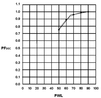
Figure 7. Graph. Approximating PF curve with two straight lines.
Figure 8 is used to calculate the pay equation transformation for use in SPECRISK when PWL is less than or equal to 50.
![]()
Figure 8. Equation. Transformation for SPECRISK when PWL is less than or equal to 50.
Entering Acceptance Quality Characteristics in SPECRISK
A key step of the setup procedure in SPECRISK is to make sure that the necessary acceptance quality characteristics have been listed for later selection as the specification profile is filled out. If SPECRISK has been used frequently for previous analyses, these may already exist. Figure 9 shows that several characteristics have been used previously, but four new characteristics pertaining to this specific example were added, beginning at the highlighted line.
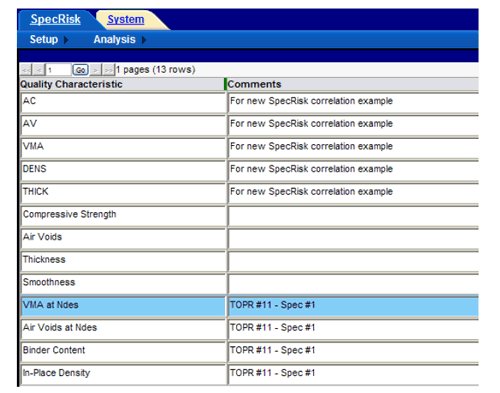
Figure 9. Screenshot. Listing acceptance quality characteristics for selection in SPECRISK.
Pay Equation Setup
The next step is to make sure the necessary pay equations are included as part of the setup procedure. In this case, figure 4 through figure 8 had not been previously entered into the particular installation of SPECRISK used for this analysis. However, the pay equation wizard makes it easy to enter these four pay equations as a single compound equation.
The first step is to enter an appropriate name for the pay equation so that it can be identified for later selection as the analysis profile is being completed, as shown in the highlighted line in figure 10. Since the same pay equation is used for all quality characteristics, only a single entry is required in this case. In figure 10, the user has also made the appropriate selections for "Quality Measure," "Pay Adjustment Units," and "Pay Equation Type" and has entered a helpful descriptive comment for future reference.

Figure 10. Screenshot. New pay equation designation with descriptive commentary.
Figure 11 shows the selections that must be made in the first window of the pay equation wizard. In the first column, "PWL" is selected as the quality measure. In the second column, the pay equation type is "Existing Equation(s)," meaning that the user has determined coefficients of the pay equation externally and will be entering them into the program. In the last column, the pay adjustment (PA) units are "Pay Factor Decimal." These three selections are all highlighted in figure 11.
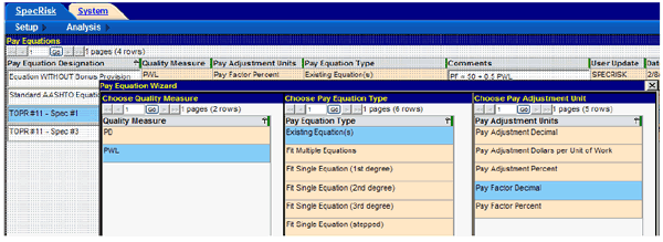
Figure 11. Screenshot. First window of pay equation wizard.
Following these selections, clicking the "Next" button at the bottom of the window (not shown) will accept these selections and proceed to the window shown in figure 12. Here, the user can create all four segments of the compound pay equation by making four selections of the linear form "B0 + B1 * X" and then entering the appropriate coefficients given by figure 4 through figure 8.

Figure 12. Screenshot. Second window of pay equation wizard.
Following the input of the equation coefficients, it can be helpful to plot the resulting pay equation to check for potential errors and discontinuities. This is accomplished by clicking the "Graph" tab just to the right of the "Setup" tab in figure 12. The "Graph" tab displays the plot shown in figure 13, in which the green and blue segments represent the linear approximations originally shown in figure 7.
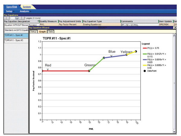
Figure 13. Screenshot. Plot of compound linear pay schedule given by figure 4 through figure 8.
When the "Graph" tab is first clicked on the screen shown in figure 12, a dialogue box indicates that there are two discontinuities in this compound linear pay schedule. However, when the dialogue box is dismissed, SPECRISK displays the complete pay schedule shown in figure 13, with no significant discontinuities. The reason for this is that the pay equation wizard only accepts four decimal places for the "B" coefficients (e.g., B1 = 0.0019 instead of the more precise value of 0.00194 in the third line of figure 12). A modification should correct this in a future edition of SPECRISK. However, as long as the plot looks visually continuous in the graph, as shown in figure 13, there will only be a minimal effect on the analysis results.
Entering Data into Simulation Profile
At this point, the user must click on "Analysis," just to the right of "Setup" at the upper left of the display to bring up the simulation profiles. If a simulation profile has previously been set up for this analysis, all the user has to do is click on it. In this example, the profile does not exist and must be created.
A profile is created by clicking on "Conventional Method Default Profile," as highlighted in
figure 14. Then, the user must right-click and select "Insert New Record Like This" in the
dropdown window, which is also shown in figure 14. It is essential to right-click either on the
highlighted line or elsewhere on the screen but not on any other simulation profile to avoid
copying the wrong simulation profile. (As noted in the SpecRisk User’s Manual, the
conventional method default profile refers to all analyses that do not employ the
expected-life method.[3])
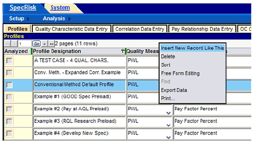
Figure 14. Screenshot. Entering a new simulation profile.
A new simulation profile line will be added at the end of the list, in this case, on page 2 of 2. The arrows near the upper left corner in figure 14 allow navigation between pages. Once viewing page 2, the user highlights the new profile and renames it as appropriate, as shown in the highlighted line in figure 15. (The expected-life method default profile appears in the top row in this figure, where it has automatically been placed in alphabetical order.)
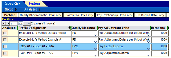
Figure 15. Screenshot. New profile located on profile page 2 and renamed.
Once the conventional method default profile has been highlighted, it is imperative that the user copy and rename this profile before attempting to make changes to it. Failure to do so will result in the conventional method default profile itself being altered, making it unavailable as a starting point for future analyses of this type. (For more details, refer to the SpecRisk User’s Manual. [3]
Figure 15 shows that a value of 1,000 has been entered for the number of iterations (replications) of the simulation process. This is usually an ample number for exploratory work and allows slower computers to run faster. For faster computers, 10,000 iterations may be used to provide more precise results. For a final run, 10,000 to 100,000 iterations may be used, which may require several hours of running time to complete the analysis when there are several quality characteristics. For extremely fast computers, SPECRISK allows a maximum of 1 million iterations.
Figure 16 shows some of the additional columns that are displayed when the screen in figure 15 is scrolled to the right. The highlighted row is the extension of the same highlighted line shown in figure 15. In most cases, it is useful to check all of the options in these columns so that they will be available after a full analysis is run.

Figure 16. Screenshot. Other possible selections on profile screen.
The next several steps involve entering the basic specification 1 information from the "Acceptance Procedure Synopsis" section. To begin, the user clicks on "Quality Characteristic Data Entry" (see figure 17). Some of the entries are typed in directly, while others are selected after clicking on the down arrows that appear in some cells.

Figure 17. Screenshot. Specification 1 quality characteristic data entry.
SPECRISK allows the entry of up to five quality characteristics for any given analysis. In figure 17, four blank rows were created and filled by first clicking the down arrows in the "Quality Characteristic" column and making appropriate selections from the dropdown menus. The appropriate pay equations, which are the same for all four quality characteristics, are selected in a similar manner in the “Pay Equation Designation” column, followed by the selection of "2-sided" as the limit type in the "Spec Limit" column. Next, the sample size of 5 and the AQL of PWL = 90 are entered in the next two columns for all four quality characteristics.
It should be noted that SPECRISK requires an entry for RQL. The user can enter values of 0 (PWL) or 100 (PD) as a default value when no RQL provision exists, but it is often useful to enter some other value of interest because the program tallies the frequency of occurrence of whatever value is entered. In this particular application, the "Acceptance Procedure Synopsis" section for specification 1 notes that an agency committee addresses instances when the sample average falls below PWL = 50 on a case-by-case basis. Therefore, a PWL of 50 has been entered in the RQL cell for each acceptance quality characteristic in figure 17. In this manner, the simulation analysis will provide an indication of how likely such an occurrence will be for specific acceptance quality characteristics at different levels of quality.
For purposes of the pay analysis, no specific action is taken when PWL < 50 occurs. Also, since there was no information available on how the agency committee might rule on such cases, it was necessary to assume that a pay level of PF = 0.75 applies down to the minimum value of PWL = 0, as shown in figure 13. Since it is likely that the committee might reject lots of extremely low quality rather than award the minimum of PF = 0.75, the simulation analysis results calculated by SPECRISK for extremely low quality may be biased on the high side.
The rest of the input proceeds in much the same manner. Because no information regarding possible correlation of the acceptance quality characteristics is available for this application, the input for “Correlation Data Entry” can be bypassed. SPECRISK defaults to a correlation of zero when no input is made. (However, there is a potential positive correlation between binder content and in-place density and a potential negative correlation between binder content and air voids. Therefore, the highway agency may attempt to check these correlations in the interest of conducting a more thorough analysis.)
Figure 17 shows that an additional column at the far right includes a checkbox for "Retest." This element does not apply for this application, nor do additional selections not shown in the figure.
In the "Acceptance Procedure Synopsis" section for specification 1, the composite pay equation shows the following weighting factors for the individual PFs:
These values must be entered into the simulation profile. This is done by clicking the "Pay Relationship Data Entry" tab and selecting “Weighted Average,” as shown in figure 18.
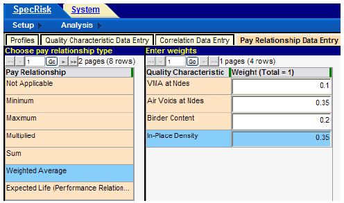
Figure 18. Screenshot. Entry of weighting factors.
The sum of the weights typed in by the user is given in the column heading in figure 18. If this sum does not equal 1.0 when the user attempts to move on to the next entry, an error message will appear, requiring the user to change one or more values.
The next tab, "OC Curves Data Entry," allows the user to enter pay levels from which a series of graphed OC curves will be produced, showing the probability of receiving these pay levels (or higher) at any level of true population quality. The pay schedule for this application is in units of decimal PF. An appropriate series of pay levels is shown in figure 19.
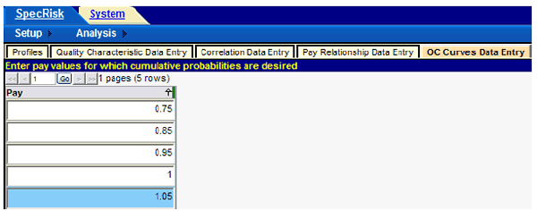
Figure 19. Screenshot. Entry of pay levels for OC curve analysis.
Preliminary Analyses
Following the input of essential entries for analysis of the specification it is customary to do a preliminary analysis by entering a few key quality level combinations rather than a complete analysis. After entering a few specific quality level combinations in the lower table, analysis is initiated by clicking "Analyze Selected," near the lower right corner of the profile screen. The results of this run are shown in figure 20. This early analysis can provide almost immediate results at quality levels of particular importance and may allow the user to spot obvious input errors.
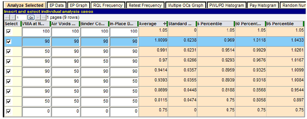
Figure 20. Screenshot. Preliminary specification 1 run using “Analyze Selected.”
For example, the highlighted row in figure 20 shows that at the AQL for which all quality characteristics are at PWL = 90, the expected (i.e., long-term average) PF of 1.0099 is almost exactly the desired value of 1.0. This indicates that a contractor who consistently performs at the AQL for all acceptance quality characteristics will receive essentially no PA in the long run and will be paid 100 percent for producing precisely at the level of quality considered to be acceptable, which is exactly as desired.
The highlighted AQL row also shows that the simulated PFs are 0.969 and 1.0433 at the 5 and 95 percentile points of the distribution, respectively. This indicates that although the acceptance procedure appropriately pays 100 percent of contract price on average when the contractor is producing at the AQL, approximately 5 percent of the time an individual PF could be at about 0.97 or lower, and similarly, about 5 percent of the time it could be at 1.04 or higher. This degree of variability is primarily due to the choice of sample size (n = 5). The use of smaller sample sizes would widen these extremes, and larger sample sizes would narrow them. The ability of SPECRISK to quantify these effects can aid highway agencies in determining suitable limits and sample sizes and can help contractors by demonstrating the effects of targeting production levels somewhat above the AQL.
In rows three through six in figure 20, one acceptance quality characteristic is set at a low quality level of PWL = 50, while the other three are held at PWL = 90. Without an explicit RQL provision to guard against low individual levels of quality, it is important to check the degree of protection afforded by the composite pay schedule itself. In rows three and four, in which the quality characteristics that have the least weight, PFVMA and PFBINDER, are set at PWL = 50, the resulting expected PFs are 0.99 and 0.97, respectively. It remains for the SHA to decide if this is a sufficient pay reduction to promote quality control efforts that will prevent these quality characteristics from dropping as low as PWL = 50 or to recoup the anticipated future costs to the agency. If not, the agency may wish to consider adding individual RQL provisions, giving the agency the option to require a retest or removal and replacement at the contractor’s expense for an appropriately defined level of poor quality.
In rows five and six of figure 20 in which the quality characteristics that have the greatest weight, PFVOIDS and PFDENSITY, are set at PWL = 50, the resulting expected PFs are both about 0.94. This may be considered high for a lot in which one of two key acceptance quality characteristics is at a quality level that might be defined as unacceptable. The benefit of this analysis is that it enables the highway agency to quantify these risks, make informed decisions about the adequacy of the acceptance procedure, and make changes when necessary.
The remaining rows in this preliminary analysis provide information about how this acceptance procedure will perform at extremely poor levels of quality. When all four acceptance quality characteristics are at PWL = 50, a level that agencies might define as RQL in all characteristics, the overall expected PF is about 0.81. At the worst possible quality level, for which all acceptance quality characteristics are at the minimum level of PWL = 0, the overall expected PF for the lot is 0.75, the minimum PF assigned by the pay schedule (see figure 4 through figure 8 and figure 13).
Ambiguity at the AQL
The formal definition of the AQL under a multicharacteristic acceptance plan is the condition at which each acceptance quality characteristic is at its respective AQL value. For this analysis, the formal AQL definition is satisfied when all quality characteristics are at PWL = 90 and, as shown in the highlighted line in figure 20, the expected PF at this quality level is almost exactly 1.0 (100 percent payment), as appropriate.
However, because of the incentive provision that makes expected payment of 100 percent at the AQL possible, there are other combinations of quality levels that can also produce 100 percent payment. In particular, it is of interest to know how low in quality any single characteristic could be while still resulting in 100 percent payment for the lot. This effect tends to be more pronounced when there are a greater number of acceptance quality characteristics used to determine the composite PF. This exploration is a trial-and-error exercise, but it can easily be accomplished with the "Analyze Selected" feature in SPECRISK.
Figure 21 shows the results of sensitivity tests for which the quality level of VMA at Ndes ranges from a maximum of PWL = 70 to the lowest possible quality level of PWL = 0, while all other quality characteristics are held fixed at PWL = 100. The top two rows have VMA set at PWL = 70 to provide an indication of how repeatable these tests are with 1,000 iterations. The values in the "Average" column represent the long-term expected PF as determined by the simulation. The two estimates of 1.0367 and 1.0358 for these two rows for a population PWL = 70 are in very close agreement, providing confidence that 1,000 iterations per run is adequate for this series of tests.
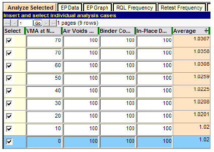
Figure 21. Screenshot. Sensitivity of acceptance procedure to VMA at Ndes quality.
As the quality level of VMA is set at lower PWL values in figure 21, the expected PFs in the last column decline accordingly. However, a possibly unexpected finding is that no matter how poor the quality of VMA is, the overall lot PF does not go below PF = 1.02. In other words, as this acceptance procedure stands, it will award a positive incentive (bonus) PF even at the worst possible quality level of VMA when all other quality characteristics are at PWL = 100. This is due both to the low weight of 0.10 assigned to VMA and the fact that there are four acceptance quality characteristics that are weighted together to obtain the composite PF.
What cannot be accounted for in this analysis is the decision of the committee that evaluates lots for which PWL < 50 is measured. However, the simulation results in figure 21 show that even for levels of VMA only slightly above PWL = 50 (when the other three quality characteristics are held at PWL = 100) for which no reevaluation is triggered, the expected PF will likely be greater than PF = 1.02. If the highway agency is uncomfortable with this result, it would be advisable to include an individual RQL provision for VMA and possibly for the other individual quality characteristics, as well.
In a sense, this result provides a check on the simulation process itself. The composite pay equation used is the same as figure 3.
When the quality level is set at PWL = 100 for binder, air voids, and in-place density, all will have the maximum PF of 1.05. When the quality level of VMA is set at PWL = 0, PF will be at the minimum of 0.75. Substituting these values in the figure 3 equation produces figure 23, with a calculated minimum composite PF of 1.02. This provides added confidence that the simulation process in SPECRISK is operating correctly.
Figure 22 shows the calculation for the lot PF when PWL = 100 for binder, air voids, and density and PWL = 0 for VMA.

Figure 22. Equation. Calculated minimum composite pay equation when PWL = 100 for binders, air voids, and density and PWL = 0 for VMA.
For the sake of thoroughness, this analysis is repeated for in-place density, which has a substantially higher weighting factor of 0.35. The results of this run, again conducted with the “Analyze Selected” feature, are shown in figure 23.
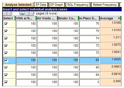
Figure 23. Screenshot. Sensitivity of acceptance procedure to in-place density quality.
This sensitivity test reaffirms the precision of these simulation runs with 1,000 iterations, as seen by the close agreement of the average values (composite PF) of 1.0168 and 1.0163 for the first two rows with density quality set at PWL = 76. Similar to figure 21 for VMA, figure 23 shows the composite PF declining as density quality declines. In this case, a composite PF of almost 1.0 is reached when the density quality level is PWL = 68. In other words, the following quality level combination can be regarded as an equivalent AQL because it produces a composite PF of essentially 100 percent:
If a SHA was concerned about paying 100 percent for this combination of quality levels, then some revision of the pay schedule would be in order. This revision might be as simple as adding appropriate RQL provisions. Repeating the type of computation made in figure 22 with PWL = 0 for in-place density results in 0.945, confirming the simulation value in the last row of figure 23.
For all practical purposes, the value of PWLDENSITY = 68 obtained from figure 23 is probably close enough for determining an equivalent AQL combination of quality levels. However, if necessary, the value can be determined more precisely using the "Analyze Selected" feature. In figure 24, all of the quality combinations have been modified to 100/100/100/68, and the simulation was rerun. The automatically ordered results in the last column of figure 24 demonstrate that PWL = 68.0 is a reasonably precise determination because the middle value in the column is equal to PF = 1.0, representing an equivalent AQL. If this had not been the case, a second trial value, using either a slightly larger or smaller value than 68.0, could be chosen and the run repeated. Each such trial would normally require less than 5 min to complete.
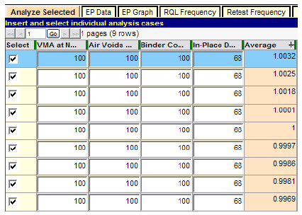
Figure 24. Screenshot. More precise determination of equivalent AQL combination.
Time-Saving Procedure
SPECRISK can be used for a full factorial experiment by simulating all combinations of quality levels in all of up to 5 acceptance quality characteristics (typically in PWL increments of 10) and by graphing most of these results as selected by the user. With a relatively large number of simulation replications, a complete analysis such as this may require several hours of computation time, depending on the speed of the computer it is run on. However, it is often possible to obtain certain key results without such a time-consuming effort. A shortcut method is described in this section.
A useful series of quality levels for analysis consists of all possible combinations of AQL and RQL values for all acceptance quality characteristics. This subset of data can be selected upon completion of the analysis, but it is also relatively easy to set up for fast results with the “Analyze Selected” procedure illustrated in figure 20 through figure 24. For specification 1, the AQL is been implied as PWL = 90 for all acceptance quality characteristics because that equates to a PF of 1.0. Accordingly, it is hoped that the forthcoming analysis will confirm that the expected composite PF for the lot will be close to 1.0, the value that is generally accepted as appropriate when the contractor produces work exactly at the AQL. An RQL has not been explicitly defined, but for purposes of this analysis, it has been defined as PWL = 50 because that is the level of quality below which the disposition of the lot is decided by an agency committee. Since there are four acceptance quality characteristics in this example, each of which may be at either of two quality levels (AQL and RQL), the total number of combinations of quality levels to be simulated is 24 = 16, a manageable number to handle with the "Analyze Selected" procedure.
The experimental design is shown in table 1, where the orderly arrangement of possible quality combinations is evident. This same arrangement is also seen in figure 25, but only the first 12 lines can be shown on the first page of the display.
| Characteristic 1 | Characteristic 2 | Characteristic 3 | Characteristic 4 |
|---|---|---|---|
| AQL | AQL | AQL | AQL |
| AQL | AQL | AQL | RQL |
| AQL | AQL | RQL | AQL |
| AQL | AQL | RQL | RQL |
| AQL | RQL | AQL | AQL |
| AQL | RQL | AQL | RQL |
| AQL | RQL | RQL | AQL |
| AQL | RQL | RQL | RQL |
| RQL | AQL | AQL | AQL |
| RQL | AQL | AQL | RQL |
| RQL | AQL | RQL | AQL |
| RQL | AQL | RQL | RQL |
| RQL | RQL | AQL | AQL |
| RQL | RQL | AQL | RQL |
| RQL | RQL | RQL | AQL |
| RQL | RQL | RQL | RQL |
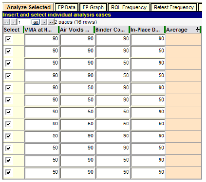
Figure 25. Screenshot. Partial display of entry of AQL/RQL combinations.
In figure 25, the AQL/RQL combinations have been entered in the order they appear in table 1, and the "Average" (expected PF) column is blank because "Analyze Selected" has not been run. After the run, the results obtained in the last column will automatically be sorted from largest to smallest, and the experimental design will no longer be easily discernible. The results of this "Analyze Selected" run are shown in figure 26 where the first 12 rows are displayed. The complete results are recorded in the original order in table 2.
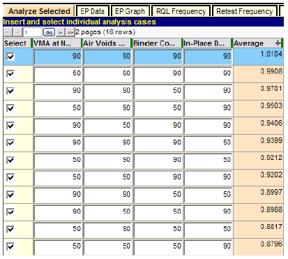
Figure 26. Screenshot. First page of display for test at AQL/RQL combinations.
| Quality Level (PWL) | Expected PF* | |||
|---|---|---|---|---|
| VMA | Air Voids | Binder Content | In-Place Density | |
| 90 | 90 | 90 | 90 | 1.0104 |
| 90 | 90 | 90 | 50 | 0.9399 |
| 90 | 90 | 50 | 90 | 0.9701 |
| 90 | 90 | 50 | 50 | 0.8997 |
| 90 | 50 | 90 | 90 | 0.9406 |
| 90 | 50 | 90 | 50 | 0.8696 |
| 90 | 50 | 50 | 90 | 0.8988 |
| 90 | 50 | 50 | 50 | 0.8295 |
| 50 | 90 | 90 | 90 | 0.9908 |
| 50 | 90 | 90 | 50 | 0.9212 |
| 50 | 90 | 50 | 90 | 0.9503 |
| 50 | 90 | 50 | 50 | 0.8817 |
| 50 | 50 | 90 | 90 | 0.9202 |
| 50 | 50 | 90 | 50 | 0.8503 |
| 50 | 50 | 50 | 90 | 0.8796 |
| 50 | 50 | 50 | 50 | 0.8118 |
*Significant to approximately two decimal places at 1,000 replications.
Table 2 provides an effective range of key combinations of results that might reasonably occur in actual field applications. When combined with the output shown in figure 21, figure 23, and the figures examining how low in quality any characteristic might be when the overall composite PF represents full payment, these results provide a reasonably thorough assessment of how the acceptance procedure and pay schedule will perform in actual practice. Specification engineers can scan this data to check for any results that stand out as inappropriate. If any results are judged unsatisfactory, the highway agency can make modifications of limits, sample sizes, retesting or RQL provisions, etc., to improve the specification.
For example, one obvious check is to make sure the specification pays an average of 100 percent at the AQL, the level that is either defined or implied to represent a satisfactory product. For this specification, this occurs when each individual quality characteristic is at an individual AQL of PWL = 90. As noted in the "Acceptance Procedure Synopsis" section, this is an implied AQL because, at this level of quality, each individual PF = 1.0 and, correspondingly, the overall composite PF = 1.0. The highlighted row in figure 26 and the first row of table 2 show that the expected PF for the simulation run was 1.0104. Since 1,000 replications were used for these runs, this is within the expected normal variability from the desired true value of PF = 1.0 and is acceptable.
While this analysis demonstrates that the contractor who performs exactly at the AQL will receive a long-term expected PF of 1.0, there is a theoretical reason that it might be slightly higher than 1.0 in this case. A perfectly linear pay relationship that includes a positive incentive provision and passes through PF = 1.0 at the AQL of PWL = 90 is known to reproduce this result as the long-term expected PF because PWL and its complement, PD are both unbiased statistical estimators. However, the pay relationship shown in figure 13 is not perfectly linear, and the lower portion that levels off at PF = 0.75 is sufficiently lenient to produce a small amount of upward bias in the upper portion of the pay schedule. Therefore, an average PF slightly above 1.0 would be an expected result, as borne out by the simulation.
At the other extreme, shown in the last row of table 2, each individual characteristic is at an RQL value of PWL = 50 and receives the minimum PF = 0.75. The expected PF in this row is 0.8118. This is larger than the minimum PF because those quality estimates that fall below PWL = 50 cannot receive anything less than the minimum PF = 0.75. Estimates that exceed PWL = 50 receive varying PFs greater than 0.75, resulting in a larger average PF. The issue here is whether a highway agency will consider it appropriate to award a high PF for such poor quality. If not, various changes may be considered, such as adding retest or RQL provisions for individual characteristics (or possibly an RQL provision based on the overall composite PF) that would give the agency the option of requiring removal and replacement of the work at the contractor’s expense, possibly pending a retest to confirm the low level of quality. The agency may also consider a more steeply declining pay relationship below PWL = 50 for the individual quality characteristics.
These two extreme cases (AQL and RQL) provide useful checks on the practicality and effectiveness of the acceptance procedure. The other rows in table 2 provide other possible combinations of quality levels from which to judge the performance of this acceptance procedure.
Full Analysis
For many agencies, the preliminary analysis may be sufficient to confirm that the acceptance procedure is working satisfactorily or to demonstrate that modifications need to be made. For those requiring more detailed information, a full analysis can be run. Full analysis usually requires additional computation time. Additionally, depending on the speed of the computer, the number of acceptance quality characteristics and the other selected user options might require several hours to complete. For extremely complex analyses, it may be practical to allow the analysis to run overnight.
For a full analysis, a minimum of 1,000 iterations is recommended for the "Profiles" screen in figure 15, and 10,000 iterations is preferred. SPECRISK will accept as many as 1 million iterations, although in most cases, that would be well beyond the point of diminishing returns. Lengthier runs, especially for multiple acceptance quality characteristics, would probably have to be run overnight on a fast computer.
It is possible to run the full analysis with a smaller number of iterations for instructional purposes to become familiar with the program. The graphs in figure 27 and figure 29 were obtained with only 100 iterations and still provide a clear picture of what SPECRISK can do.
Whereas the preliminary analysis in figure 26 and table 2 provide the expected PFs at selected key combinations of quality levels, the EP graph in figure 27 provides this same information over the entire range of possible quality levels. In the upper left corner of figure 27, the user has chosen to display the EP graph for the composite (overall) PF for the lot. This feature also has the capability of displaying graphs for individual quality characteristic PF by selecting the quality characteristic from the dropdown and clicking "Refresh." An important finding, shown by the red line, is that the expected PF at the AQL (in this case, where each quality characteristic is at PWL = 90) is almost exactly 1.0, as desired.
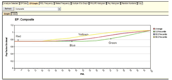
Figure 27. Screenshot. EP graph for composite expected payment.
The composite EP graph in figure 27 has a limitation where in order to present this information for multiple acceptance quality characteristics in a two-dimensional plot, it requires that all acceptance quality characteristics are simultaneously held at the quality levels shown on the x-axis. This is usually sufficient to obtain an impression of how the pay schedule will perform, but it does not provide all details. The actual analysis that is run by SPECRISK includes all combinations of all quality levels, usually in PWL increments of 10. If desired, the complete array of results is obtainable by clicking the “EP Data” tab shown in figure 28.
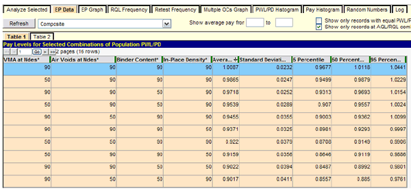
Figure 28. Screenshot. Filtered array of output data for AQL/RQL combinations.
In figure 28, table 1 is shown, and the user has made two selections: "Composite" at the upper left and "Show only records at AQL/RQL combinations" at the upper right. By clicking "Refresh," the user has employed one of several selectable data filters to reduce 14,641 rows of simulation data to just 16 rows of interest on two pages of display. The "Table 2" tab provides additional ways to filter the raw output data but was not used in this analysis.
The output in figure 28 shows the same selection of AQL/RQL combinations that are shown in table 1 and table 2, which were obtained more quickly with the "Analyze Selected" feature shown in figure 26. In figure 26 and figure 28, the combination of all quality characteristics at their respective AQL values is highlighted. The expected composite PF in the two highlighted rows are 1.0104 and 1.0087, which is well within the degree of agreement that would be expected for two separate simulation runs. However, since PF = 1.0104 was obtained with 1,000 iterations for the "Analyze Selected" run while only 100 iterations were used to demonstrate the full analysis, the value of 1.0104 is likely to be closer to the correct value. (In both cases, this confirms the desired value of PF = 1.0 at the AQL.)
Figure 29 shows the multiple OCs graph, which is another optional output graph that will be of interest to both SHAs and the contractors. In this figure, the user has selected the composite graph, which pertains to the overall composite PF for the acceptance lots.
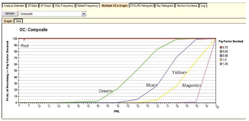
Figure 29. Screenshot. Multiple OCs graph.
The legend in figure 29 identifies the OC curves corresponding to the input values entered by the user in figure 19. For example, the yellow line (PF = 1.0) indicates that a contractor producing at an AQL of PWL = 90 will receive PFs of 1.0 or higher about 65 percent of the time. However, if the contractor produces above an AQL at PWL = 95, the probability of obtaining the maximum PF = 1.05 is about 50 percent, and the probability of obtaining PF = 1.0 or higher is about 80 percent (see the magenta line). The red line in figure 27 shows that a contractor who produces at an excellent quality level of PWL = 95 would expect an average PF of about 1.02 or 1.03. This is confirmed to be about PF = 1.03 by running “Analyze Selected” again and including an additional row for PWL = 95 in all acceptance quality characteristics, as shown in figure 30. The AQL row with all quality characteristics at PWL = 90 was also included in this run to confirm the slight upward bias at an AQL of about PF = 1.01.

Figure 30. Screenshot. "Analyze Selected" run with all quality characteristics at PWL = 95.
There are several additional tabs in figure 28 that may be selected to obtain additional graph and table displays. Not all will be required for all analyses, but collectively, they indicate the wide range of output options in SPECRISK. For additional examples, see the SpecRisk User’s Manual and the other specification analyses in this report.[3]
Analysis Summary and Conclusions
This analysis accomplished two goals. First, it demonstrated the amount that can be learned about an acceptance procedure and pay schedule using just the "Analyze Selected" feature in SPECRISK. This method can result in a considerable time savings for more complex acceptance procedures with several acceptance quality characteristics and demonstrates the ease with which some of these analyses can be done on computers with modest capacity and speed. Second, it revealed interesting findings about a moderately complex acceptance specification based on four acceptance quality characteristics. A multicharacteristic analysis such as this would not have been feasible before SPECRISK was developed.
Significant procedures and findings are as follows:
SPECIFICATION 2
Acceptance Procedure Synopsis
Type of Specification
Acceptance Quality Characteristics
Correlation of Acceptance Quality Characteristics
Lot Size Definitions
Sample Sizes
Statistical Quality Measure
Individual Pay Equations (PA as Decimal)
![]()
Figure 31. Equation. Individual pay equation for density.
Where:![]()
Figure 32. Equation. Individual pay equation for air voids.
Where:
![]()
Figure 33. Equation. Individual pay equation for thickness.
Where
Composite Pay Equation
AQL/RQL
Pay Equation Transformations and Assumptions
To analyze this specification with SPECRISK, transformations and assumptions must be made. For example, the specification implies that the individual PFs are directly additive to obtain the overall PA for the project. This is the logical approach, and no other approach is explicitly stated. Although none of the individual PAs may match up exactly with any other in terms of precise pavement locations, collectively, they account for the entire paved area of the project. SPECRISK accommodates this procedure, but the actual analysis assumes that each set of tests for different quality characteristics applies to the same lot. It is believed, but has not been demonstrated, that this assumption of common lot sizes has little if any effect on the final results.
Density
The equation for density in figure 31 is already in a form that can be accommodated by SPECRISK, but it must be noted that this applies for 50 < PWL ≤ 100. For PWL < 50, PA = -0.16 (constant). Both segments of this compound linear pay equation will be entered into SPECRISK, as will be explained in the following sections.
Although an RQL consequence is not specified explicitly, SPECRISK requires that a value be entered into the program. Entering PWL = 50 provides a frequency count of estimates for which PWL < 50, which may trigger reevaluation by the SHA.
Air Voids
The equation for air voids in figure 32 must be modified slightly. By using the equation in figure 34, figure 32 can be rewritten as figure 35, which is in the same form as figure 31.
![]()
Figure 34. Equation. Modification of individual air voids equation.
![]()
Figure 35. Equation. Further modification of individual air voids equation.
This applies specifically for 50 < PWL = 100. For PWL < 50, a second segment described by PA = -0.12 is required, both of which will be entered into SPECRISK.
As previously noted, PWLLSL or PWLUSL < 50 or PWLVOIDS < 50 will trigger a reevaluation by the agency, which might lead to a requirement to remove and replace the affected material. If left in place, the minimum PA = -0.12 is applied. Unfortunately, SPECRISK does not have the capability to perform the first of these two tests, so only the second one can be included in these analyses. It is believed that this has little effect on the final results.
There is also a special t-test requirement for air void tests. This is another refinement that the SPECRISK software cannot duplicate, so it is necessary to assume that the effect will be minor.
Thickness
For the thickness acceptance procedure, an equivalent RQL provision is in effect. When PWLTHICKNESS < 50, a full-width overlay is required, after which new cores are taken and the calculations are repeated (the original thickness results are discarded). After the overlay is placed, it is almost certain that the lot will be acceptable for thickness, although no incentive adjustment is permitted in this case. Therefore, full payment is likely, and the effective PA is simply the added cost to the contractor of the required overlay. This corresponds to a negative PA, and for lack of a better estimate, the minimum value of PA = -0.27 from figure 33 is used.
Figure 33 for the thickness PA is the same as figure 35 for the modified air voids PA. SPECRISK can accommodate this, but it has to be entered as a distinct equation because of the constant PA = -0.27 for PWL < 50.
From a sampling standpoint, however, the retest used is not the type of retest assumed in SPECRISK. The assumption is that a second set of samples is taken from the same lot, which may then be either combined with the first set or used by itself to make the final determination of lot acceptance. Since the specification under analysis requires that an overlay be placed before the second set of measurements is obtained, the retesting is not performed on the original population.
Additionally, there are two special outlier requirements for thickness of individual core lengths (see synopsis above) that can alter the standard calculation of some of the Q statistics and can also lead to isolated overlay requirements. Although these occurrences are expected to be relatively rare, the outlier requirements cannot be accommodated by SPECRISK and will have to be ignored.
There appears to be no easy way around these SPECRISK limitations. However, the assumptions outlined will be used to provide an instructive example of the capabilities of the software. It is also possible that since these problematical situations tend to occur only when poor to very poor quality is received, the analysis will produce useful results for the levels of quality that would normally be produced.
Entering Quality Characteristics in SPECRISK
A key step of the setup procedure in SPECRISK is to make sure that the necessary quality characteristics have been listed for later selection as the specification profile is filled out. If SPECRISK has been used frequently for previous analyses, these may already exist. Figure 36 shows that several characteristics had been used previously, but, three new characteristics pertaining to this specific example were added. The new characteristics begin at the highlighted line with the exception of the generic characteristic for smoothness.
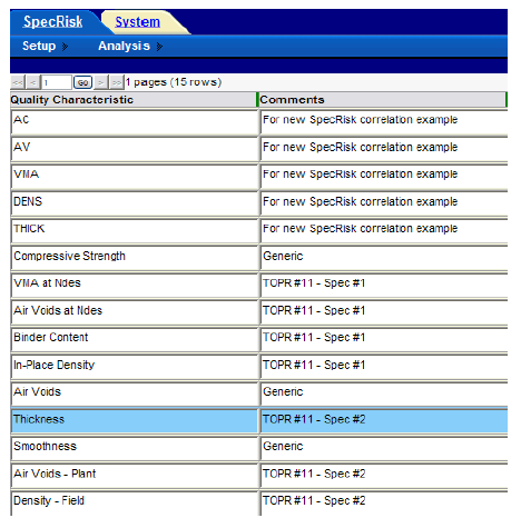
Figure 36. Screenshot. Quality characteristics for selection in SPECRISK.
Pay Equation Setup
The next step is to make sure the necessary pay equations are included as part of the setup procedure. In this case, none of the above pay equations had been previously entered into this particular installation of SPECRISK. However, the pay equation wizard makes it easy to enter these three pay equations as linear compound equations.
Density
Figure 35, the density pay equation, is shown in figure 37 as it appears after entry into the pay equation wizard.

Figure 37. Screenshot. Input of compound linear pay equation for density.
Following the input of the equation coefficients, it can be helpful to plot the resulting pay equation to check for potential errors and discontinuities. This is accomplished by clicking the "Graph" tab, which displays the plot shown in figure 38, in which the green and red segments represent the equation segments defined in figure 37.
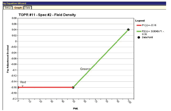
Figure 38. Screenshot. Plot of density pay schedule with minimum PA = -0.16.
Air Voids and Thickness
The pay schedules for air voids and thickness are entered in the pay equation wizard in the same manner as shown for density in figure 37. The graphs for the air void and density pay equations are shown in figure 39 and figure 40, respectively. (The scales on the ordinates are not the same.)
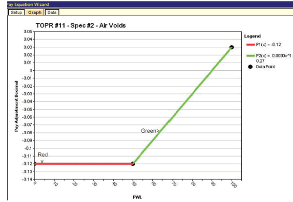
Figure 39. Screenshot. Plot of air voids pay schedule with minimum PA = -0.12.
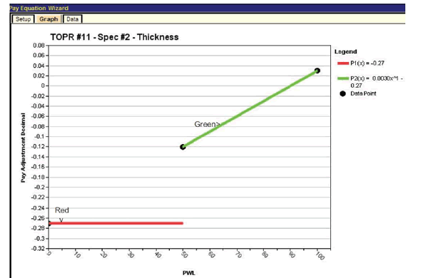
Figure 40. Screenshot. Plot of thickness pay schedule with minimum PA = -0.27.
When the "Graph" tab is selected in figure 40, SPECRISK will display a warning message noting that there is a discontinuity in this pay equation. In this particular case, the discontinuity is intentional to assess a negative PA of -0.27 whenever the original estimate of PWL < 50 necessitates an overlay and new cores from that overlay again produce PWL < 50 (see the thickness requirements in the "Pay Equation Transformations and Assumptions" section).
Entering Data into Simulation Profile
At this point, the user must click on "Analysis" to bring up the simulation profiles. If a simulation profile has previously been set up for this analysis, all the user has to do is click on it. In this example, the profile does not exist and must be created.
A profile is created by clicking on "Conventional Method Default Profile" (see figure 41). Next, the user must right-click and select "Insert New Record Like This" in the dropdown window. It is essential to right-click either on the highlighted line or elsewhere on the screen but not on any other simulation profile to avoid copying the wrong simulation profile. (As noted in the SpecRisk User’s Manual, the conventional method default profile refers to all analyses that do not employ the expected-life method.[3])
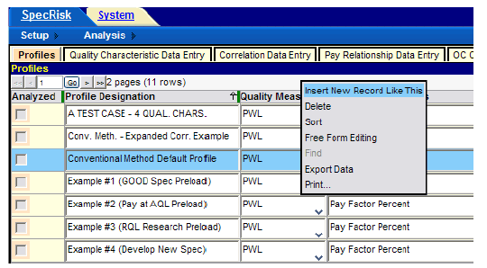
Figure 41. Screenshot. Entering a new simulation profile.
This action causes a new simulation profile line to be added at the end of the list, which, in this case, appears on page 2 of 2. The means to navigate between these pages is provided near the upper left corner in figure 41. Once there, the user highlights the new profile and renames it as appropriate, as shown by blue highlight in figure 42. (Note that "Expected-Life Method Default Profile" appears in the top row in this figure, where it has automatically been placed in alphabetical order.)
Once the Conventional Method Default Profile has been highlighted on the “Profile” screen, it is imperative that the user copy and rename this profile before attempting to make changes to it. Failure to do so will result in the Conventional Method Default Profile being altered and unavailable as a convenient starting point for future analyses of this type.
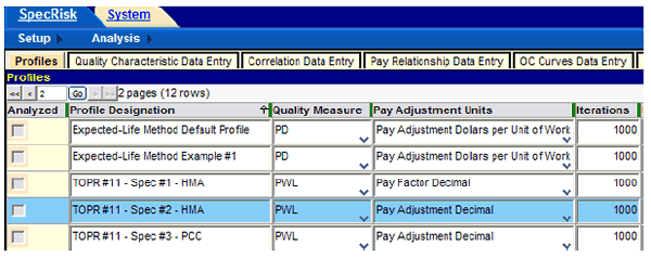
Figure 42. Screenshot. New profile located on profile page 2 and renamed.
Initial setup for simulation profile follows the same steps described in the section, "Entering Data into Simulation Profile" for specification 1. The user creates a copy of the conventional method default profile and renames it to reflect the details of specifications 2. As with specification 1, 1,000 iterations are used and all the output options are selected.
The next several steps involve entering the basic information from the specification 2 "Acceptance Procedure Synopsis" section. To begin, the user clicks on "Quality Characteristic Data Entry" (see figure 43). Some of the entries are typed in directly, while others are selected by clicking on the down arrows that appear in some cells.

Figure 43. Screenshot. Specification 2 quality characteristic data entry.
The three quality characteristics used in this example appear in the second column in figure 43. The appropriate pay schedules have been selected and are shown in the third column. After that, the types of limits (one-sided or two-sided) have been selected, followed by the sample sizes and AQLs and RQLs in units of PWL. As previously noted, the AQL values of PWL = 90 have been inferred because the acceptance procedure produces a zero PA (PF equal to 100 percent) at PWL = 90. SPECRISK requires an entry for RQL. Even if one is not explicitly defined, this feature is useful because it allows the simulation program to count the frequency of occurrence of any particular PWL level of interest. In the case of thickness, PWL < 50 is the equivalent of an RQL provision because the affected area must be overlaid and retested when the initial tests indicate that level. Consequently, the "Retest" box has been checked in figure 43.
When the "Retest" box is checked, additional input is required, as shown in figure 44. Since the acceptance procedure requires an overlay when the thickness PWL < 50, the retest limit is entered in the "Retest Trigger PWL/PD" column. After the overlay is placed, it is resampled with a sample size of n = 5, and the original test results are discarded. Therefore, "5" is entered in the last column, and "Discard Original" is selected.

Figure 44. Screenshot. Additional input required for retest provision.
The next entry tab, "Correlation Data Entry," can be bypassed. Because no information regarding possible correlation of the quality characteristics was provided for this example, it will be assumed that all correlation values are zero, the default in SPECRISK.
The "Pay Relationship Data Entry" tab is selected next. Because the individual PAs are directly summed for this specification, the appropriate selection is "Sum" in the "Pay Relationship" column, as shown in figure 45.
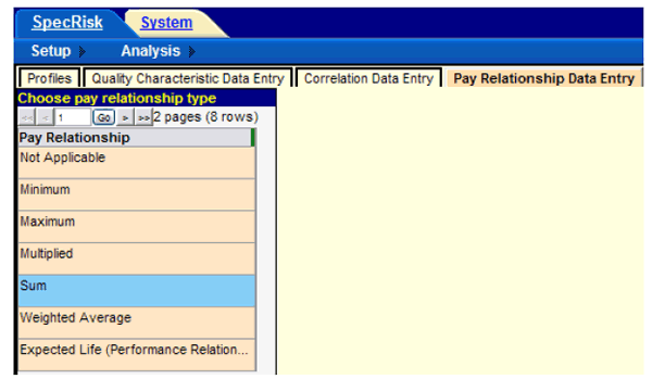
Figure 45. Screenshot. Selection of sum for the pay relationship.
The "OC Curves Data Entry" tab allows the input of user-selected levels of PA for which OC curves will provide the likelihood of achieving this level of adjustment at various levels of asconstructed PWL. This result will be accessible by selecting "Multiple OCs Graph" in the lower section of this screen after the analysis has been run. Figure 46 shows that the user has entered five different levels of PA for this analysis.
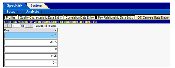
Figure 46. Screenshot. Entry of PA levels for OC curve analysis.
The remaining input tab on the profile screen is "Simulation Points Data Entry." By default, SPECRISK analyzes all possible combinations of quality levels among the selected quality characteristics in PWL increments of 10. This usually provides a fairly complete picture of the performance of the acceptance procedure over the entire range of possible quality levels, so no additional increment levels are added. However, this analysis procedure can be modified by the user if desired.
Preliminary Analyses
Following the input of essential entries for analysis of the specification, it is customary to perform a preliminary analysis by entering a selected key quality level combinations rather than a complete analysis. After entering the combinations, analysis is initiated by clicking "Analyze Selected," near the lower right corner of the profile screen. The results of one of these runs are shown in figure 47. This early analysis can provide almost immediate results at quality levels of particular importance and may also allow the user to spot obvious input errors.
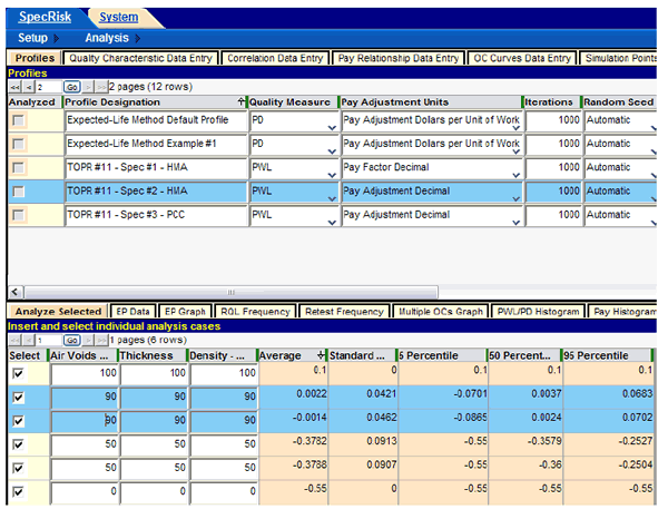
Figure 47. Screenshot. Preliminary specification 2 run using "Analyze Selected."
One technique that is frequently used when running "Analyze Selected" is to run duplicates of some combinations of quality levels to get an impression of how repeatable (e.g., reliable) the results are. Since the analysis technique used in SPECRISK is computer simulation, it is normal for successive runs (using automatic random seed numbers) to give slightly different results, and the results will be more variable when a smaller number of iterations are used. This particular simulation, using three quality characteristics, is considerably less computationally intensive than simulations using four or five characteristics. Thus, it was possible to obtain results quickly using 1,000 iterations for these trial runs (as indicated in the upper table in figure 47). By using 1,000 iterations, it is common for the results to be in good agreement.
One combination of particular interest occurs at the formal AQL, when each individual quality characteristic is at its respective AQL. Since each individual pay equation produced a PA of zero, (i.e., 100 percent payment) at PWL = 90, this is the inferred AQL for all three quality characteristics. This level of quality has been duplicated in the lower table in figure 47, as indicated by the two highlighted rows. Both runs at this level produced almost exactly the desired average PA of zero. Therefore, this run provided two important pieces of information— the acceptance procedure properly accepts AQL quality at full payment, and the result appears to be repeatable.
A similar test was run in the fourth and fifth analysis rows in figure 47. In this case, all three characteristics were set at PWL = 50, which would generally be regarded as a very poor quality lot. The results are consistent, with both being close to a PA = -0.38. The SHA must judge if the amount of payment withheld is appropriate for this level of quality.
Another common test sets the independent variables at their extremes, where it is often possible to deduce what the correct result should be. In the first analysis row in figure 47, all quality characteristics have been set at their maximum possible value of PWL = 100. The equations in figure 31 through figure 33 produce incentive PAs of +0.04, +0.03, and +0.03 when all characteristics are at PWL = 100, respectively. Since these PAs are additive, the net overall PA is +0.10, as correctly reported in figure 47.
At the other extreme, the last row in figure 47 shows all quality characteristics set at the minimum, PWL = 0. In this case, density and air voids receive minimum PAs of -0.16 and -0.12, respectively. For thickness, the assumption was that when an immediate overlay is required at the time of construction because the first series of tests produced an estimate of PWL < 50, a similar failure of the second series of tests would receive the equivalent of a PA of -0.27 (assumed cost of the overlay). Therefore, when all three quality characteristics are at PWL = 0, the overall PA is calculated as PA = -0.16 + -0.12 + -0.27 = -0.55, as shown in figure 47.
These results are a strong indication that the inputs have been entered properly, and it is reasonable to conclude that the software is performing the analyses correctly. It is appropriate to proceed with additional preliminary analyses of interest.
This specification has a virtual RQL provision in that when PWL < 50 is estimated for any quality characteristic, the agency has the option to reevaluate (density and air voids) or require an immediate overlay (thickness). A SPECRISK analysis can determine what the typical PA will be when quality levels are poor but not quite poor enough to trigger these provisions. To address this scenario, the run in figure 48 was performed. For this test, each characteristic was set at a low quality level of PWL = 50, while the other two were set at the maximum quality level of PWL = 100. As in the previous test, the quality level combinations were duplicated, and all the results appear to be repeatable. The PAs when individual characteristics are set at PWL = 50 are approximately -0.04, -0.06, and -0.08 for air voids, thickness, and density, respectively. Again, the SHA will have to decide if this provides adequate protection against low levels of quality.

Figure 48. Screenshot. Comparison of individual low levels of quality.
As shown in figure 48, the severity of PA increases in the order of air voids, thickness, and density. Another series of tests is necessary to determine why density is the most severe, at approximately PA = -0.08, when thickness has the lowest possible minimum PA at -0.27 versus -0.16 for density and -0.12 for air voids. In these runs, the individual characteristics under test are held at PWL = 0, while the other two characteristics are again held at PWL = 100. The results are shown in figure 49. Since all the previous repeatability checks showed excellent agreement, they were omitted from this series of tests.

Figure 49. Screenshot. Severity investigation with test PWL = 0 and controls PWL = 100.
Figure 49 shows the expected result, with each characteristic achieving its individual minimum PA plus the combined maximum incentive of the other two. For example, the maximum disincentive for thickness is -0.27, while the maximum incentive from air voids and density is the sum of 0.03 + 0.04, producing a total of -0.20, as shown in the third row of figure 49.
This analysis confirms the expectation that, for extremely poor quality, the thickness requirement dominates. But it is also useful to consider what the results in figure 49 imply about the application of this acceptance procedure. There does not appear to be a serious problem with the third row in the figure because whenever the original tests for thickness produce PWL < 50, an immediate overlay is required. Also, there should not be a major problem with air voids or thickness in the first two rows provided that the agency exercises either the option to negotiate removal and replacement or a lower PA. (See notes in the "Acceptance Procedure Synopsis" section for specification 2.)
An additional series of tests can provide a reasonableness check of the preliminary results. For these tests, each individual quality characteristic is varied throughout the complete range of possible quality levels while the other two are held at the AQL of PWL = 90. These results are presented in figure 50 through figure 52 for air voids, thickness, and density.
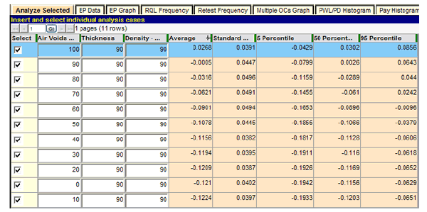
Figure 50. Screenshot. Extended test of air void PAs.
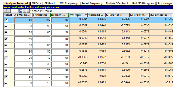
Figure 51. Screenshot. Extended test of thickness PAs.
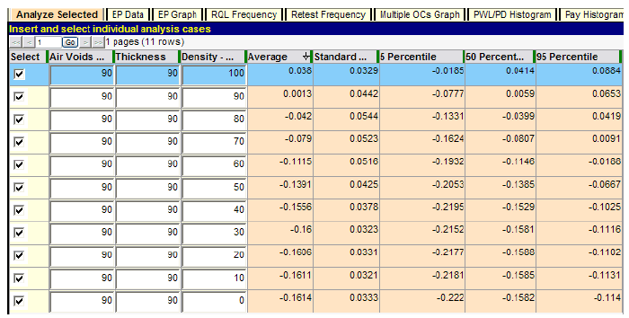
Figure 52. Screenshot. Extended test of density PAs.
Several observations can be made from this group of test runs. As each quality characteristic is decremented by PWL = 10 while both remaining characteristics are held constant at the AQL of PWL = 90, the expected average PA decreases steadily until its individual minimum PA is approached. Beyond that, the decreases are very small and due partly to the small variability of the sum of the other two PAs, which randomly vary both positively and negatively around zero because the other two characteristics are held constant at their respective AQLs. As a result, it is possible on any particular run for the lot PA to reach a minimum just slightly below the minimum PA for the characteristic under test, and the last two or three rows can be out of order due to random chance, as shown in figure 50 and figure 51.
The three figures also show that at the point at which all characteristics are at the AQL level of PWL = 90, the resultant expectant PA (average) is almost exactly zero (full payment). The fact that these small values may be either positive or negative further attests to the unbiased nature of this acceptance procedure in awarding full payment of PA = 0 at the AQL.
Ambiguity at the AQL
As previously noted, the condition at which all quality characteristics are simultaneously at their respective AQL values can be regarded as a formal definition of an AQL lot for which full payment should be awarded. However, when analyzing multicharacteristic acceptance procedures, there are many combinations of quality levels that will also produce full payment.
For example, if HMA pavement were to fall just short of meeting the design requirement of PWL = 90 for thickness (e.g., PWL = 85), but compaction exceeded the design requirement (e.g., PWL = 95), it is possible that the superior quality in compaction could make up for the mild deficiency in thickness. In fact, this offsetting property can be observed in many design procedures. When a nomograph was the standard procedure for determining the design thickness of PCC pavement, it could easily be demonstrated that there were many different combinations of compressive strength and thickness that would yield the design value of allowable load repetitions.
To study the performance specification 2 in terms of this offsetting property, a series of tests can be run for which each quality characteristic in turn is cycled from its AQL downward as the other two characteristics are held at the maximum quality level of PWL = 100. In this manner, it is possible to discover just how low in quality each characteristic can go with the lot as a whole still receiving full pavement. The first such test is for air voids, as shown in figure 53.
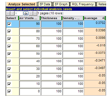
Figure 53. Screenshot. Determination of critical level of air voids quality.
In figure 53, air void quality is tested over the complete range from its AQL of PWL = 90 down to PWL = 0 to provide a complete illustration of the trial-and-error process to determine the quality level at which the lot PA is exactly zero (full payment). This run shows that full payment occurs at a PWL level just below 70. To establish this value more precisely, a follow-up run could be made, as shown in figure 54.
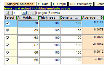
Figure 54. Screenshot. Precise determination of critical level of air voids quality.
According to figure 54, full payment (PA = 0) occurs at a point close to an air voids quality level of PWL = 67. This extreme combination of quality levels (PWL = 67/100/100) is rare but possible, and the SHA must decide whether or not full payment is acceptable for this level of lot quality. If the specification has had a history of working well, this level of risk may be acceptable. Similar follow-up runs for thickness and density are shown in figure 55 and figure 56, respectively.
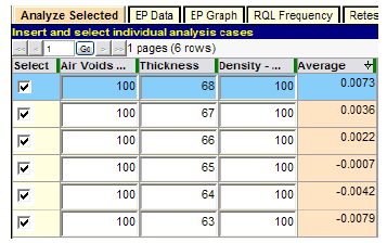
Figure 55. Screenshot. Determination of critical level of thickness quality.
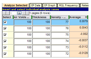
Figure 56. Screenshot. Determination of critical level of density quality.
Figure 55 shows that thickness quality might be as low as PWL = 65, and the lot could still receive essentially full payment (PA = 0). Figure 56 shows that full payment could also occur when density quality is as low as PWL = 75. However, both of these results can only occur when the other two quality characteristics are at perfect levels of PWL = 100, which would be relatively rare. Therefore, if the acceptance procedure has had a history of encouraging good quality on the part of the construction industry, and the SHA has been reasonably satisfied with it, these risks may not be of serious concern.
Time-Saving Procedure
As previously noted, SPECRISK can be used for a full factorial experiment by simulating all combinations of quality levels in up to five quality characteristics. However, it is possible to obtain certain key results without such a time-consuming effort by using the “Analyze Selected” procedure.
For specification 2, the AQL has been implied as PWL = 90 for all quality characteristics because that equates to a PA = 0. An explicit RQL consequence has been defined for thickness of PWL < 50, at which an overlay is required. For air voids and density, the RQL has been taken to be PWL < 50 because that is the level of quality below which the SHA could decide to reject the work. Since there are three quality characteristics in this example, each of which may be at either of two quality levels (AQL and RQL), the total number of different combinations of quality levels to be simulated is 23 = 8, a manageable number with the "Analyze Selected" procedure. The experimental design and the results of this analysis are shown in figure 57.
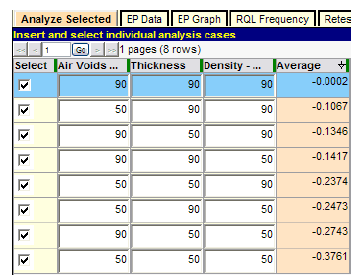
Figure 57. Screenshot. Test with all AQL/RQL combinations.
Figure 57 demonstrates that when all three quality characteristics are at an AQL of PWL = 90 (highlighted row), the resulting average PA is essentially zero, representing full payment for quality precisely at the level specified. The next three lines represent moderately defective quality for which one of the quality characteristics is at the presumed RQL of PWL = 50, while the other two are at the AQL producing similar PAs ranging approximately from -0.11 to -0.14. The next three lines represent more seriously deficient quality for which two of the quality characteristics are at PWL = 50, while the other remains at PWL = 90, producing larger pay reductions ranging approximately from -0.24 to -0.27. Finally, the last row represents extremely poor quality for which all characteristics are at the presumed RQL value of PWL = 50, resulting in a still more severe pay reduction of nearly -0.38. These results appear to be generally consistent in that they assess increasingly greater pay reductions for increasingly poorer quality and they provide the highway agency with the information to decide if the pay schedule is performing in a manner the agency considers satisfactory.
On the positive side of the pay schedules, figure 58 shows the level of incentive PA the qualityconscious contractor can receive by controlling production at or near the maximum quality level of PWL = 100. Although no lot can achieve complete perfection as indicated by a PWL level of 100 percent, it is possible (and common) for good quality lots to test out at PWL = 100 because of random sampling variability. Whenever this occurs, the contractor will receive an expected PA = 0.1, which is a positive incentive payment of 10 percent (see figure 58).

Figure 58. Screenshot. Demonstration of positive incentive provision.
Full Analysis
For many agencies, the preliminary analyses may be sufficient to confirm that the acceptance procedure is working satisfactorily or to demonstrate that modifications need to be made. For those desiring more detailed information, a full analysis can be run. One major advantage of a full analysis is that it provides access to the many graphical and tabular displays of data that SPECRISK can provide. Figure 59 shows the various types of output that can be selected from the "Profile" screen, and it is usually best to check all of them when running a full analysis.

Figure 59. Screenshot. Graphical and tabular output options in SPECRISK.
The check boxes in figure 59 represent most of the tabular and graphical output available as follows:
These output options can be useful for various applications of the software depending on the type of analysis being performed. The following list is an effort to categorize the usefulness of the various features for specific applications:
Specification analysis by highway agencies and/or contractors:
Further study by research agencies:
Program validation by software specialists:
Accordingly, this analysis will be completed using those features most appropriate for this particular specification. A full analysis is initiated by clicking on the "Analyze" button in the upper right section of the "Profile" screen. Up until now, the "Analyze Selected" button in the lower right of this screen has been used for highly selective analyses. If the user attempted to access any of the various graphical or tabular outputs before running a full analysis, a warning message would appear on the screen indicating that the full analysis must be run first.
The most important graph for SHAs (and possibly also for contractors) is the EP graph, which depicts how payment is related to quality delivered. The graph produced by the full analysis is shown in figure 60.
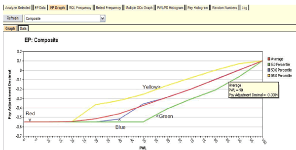
Figure 60. Screenshot. EP graph available with full analysis.
The red line represents the average (or expected) PA. The label at the upper left indicates that it represents the composite (or overall) combined PA resulting from the PAs for the individual quality characteristics. This graph has been displayed by clicking on the down arrow at the upper left of this figure, selecting "Composite" from the dropdown, and then clicking "Refresh." This same graph can also be displayed for each of the individual characteristics, and they would be similar in form because each contributes in an additive fashion to the overall combined PA.
The red line in figure 60 shows the gradual increase from the minimum PA of -0.55 at PWL = 0 up to the maximum PA of 0.1 at PWL = 100. This graph allows both the highway agency and its contractors see exactly how the acceptance procedure will perform and what the consequences of both good and poor quality control are likely to be.
For example, highway specification engineers can see that this specification awards 100 percent payment at an AQL of PWL = 90. Figure 60 also illustrates the hover feature of SPECRISK whereby a quantitative reading can be obtained from the graph by hovering the cursor close to the point of interest. In this case, a PA of -0.0004 is expected at an AQL of PWL = 90.
With this information, highway agencies can judge if the acceptance procedure is both effective and fair, and contractors can see the benefits of targeting quality levels at or above the AQL. The highway agency has an interest in confirming that the rate at which payment declines as the quality drops below the design quality level is both effective and appropriate. This graph also communicates to the contractor the seriousness of specifications of this type and that poor quality is likely to be detected and assessed appropriate pay reductions. However, this also illustrates the potential monetary benefits available to the contractor who exercises good quality control and produces work at or above the AQL
Figure 61 shows how the multiple OCs graph can provide more information on this subject. As in figure 60, the user has selected the composite analysis. The legend lists several PA levels previously entered by the user, and the central blue line represents full payment (PA = 0) in this case.
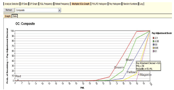
Figure 61. Screenshot. Display of multiple OCs graph.
Using the hover feature shows that work produced at an AQL of PWL = 90 is expected to receive a PA of zero or better (i.e., no adjustment or some degree of positive payment) about 51 percent of the time. This also means that about 49 percent of the time there will be some degree of pay reduction, which is not as bad as it might appear. In reality, the contractor who can successfully produce at that AQL can expect to receive 100 percent payment in the long run because the positive and negative PAs will cancel out equally at the AQL. This result illustrates why it is necessary to have some degree of incentive provision in order for any acceptance procedure of this type to fairly pay full price for work that is consistently at the AQL.
This graph also provides guidance to contractors who might prefer to control production so that there will more incentives than disincentives throughout the course of a project. For example, figure 61 shows that if the contractor could reasonably control production around PWL = 95, the probability of receiving full payment would increase from 51 to about 75 percent, and the likely average PA would be about 0.05. If it were relatively easy for a contractor to achieve this level of quality, it might be a profitable strategic move to operate somewhat above the AQL. In any case, SPECRISK has provided information to help make this decision.
The one quality characteristic for which there is an explicit RQL requirement is thickness. A result of PWL < 50 on the original set of tests leads to the requirement of an immediate overly at the time of construction. The retest frequency graph allows users to determine how often this requirement might be triggered at various levels of production quality. To do so, view the graph, select "Thickness," and refresh the image. The results are shown in figure 62.
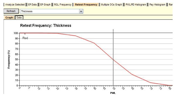
Figure 62. Screenshot. OC curve for thickness retest frequency graph.
When the true lot quality level is PWL = 50, the probability that an overlay will be required is close to 50 percent, which is an expected result. What this OC curve provides that is not intuitive are the probabilities of requiring an overlay at other levels of lot quality. For example, as long as the thickness lot quality is PWL = 80 or higher, there is almost no chance of triggering the overlay requirement. In the other direction, if the lot quality is truly PWL = 30, there is about a 95 percent chance of requiring the overlay. As noted elsewhere, certain necessary assumptions may cause the results at lower quality levels to be suspect, and this could affect the thickness results at PWL = 30. The highway agency must decide if these risks are acceptable, but the analysis has at least provided a quantitative basis for the decision.
As previously noted, there are several additional output features that may be of interest. While not used for this particular analysis, they may be found in the SpecRisk User’s Manual or elsewhere in this report. [3]
Analysis Summary and Conclusions
This analysis accomplished multiple goals. First, although SPECRISK can handle a wide range of acceptance procedure requirements, there will occasionally be some that have specialized features that do not fit exactly into the analysis mode used by this software. This does not necessarily mean that these analyses cannot be attempted, nor that useful information cannot be obtained. Specification 2 has provided an object lesson of the type of thinking required to recognize limitations and find ways to work around them. For example, while certain assumptions were required to allow the software to run, many of the problematical issues occurred primarily at low levels of quality. Therefore, it was theorized that the results obtained at higher levels of quality (at or near the AQL, the region in which most of the work will hopefully fall) can be expected to be reasonably accurate. Also, this analysis, like the analysis of specification 1, illustrated how much useful information can be obtained relatively quickly with the "Analyze Selected" feature of SPECRISK. Finally, this analysis provided a good overview of the many capabilities this software has to offer.
Significant findings were as follows:
A duplicate of this analysis with the thickness quality characteristic excluded is presented in appendix B of this report.
SPECIFICATION 3
Acceptance Procedure Synopsis
Type of Specification
Quality Characteristics
Statistical Quality Measure
Lot Pay Equation (Both Characteristics)
The lot pay equation is shown in figure 63 as follows:
![]()
Figure 63. Equation. Lot pay equation for compressive strength and thickness.
Where:
PWLCOMPSTR = PCC compressive strength.
PWLTHICK = PCC pavement thickness.
When PWLCOMPSTR = PWLTHICK = 100, the maximum PA is 0.06. Similarly, when PWL < 50, it is set equal to 50, and the minimum PA is -0.24.
AQL/RQL
Sample Sizes
Pay Equation Transformation
To analyze the pay equation presented in figure 63 with SPECRISK, it must be converted into separate pay equations for strength and thickness, with the overall composite result expressed as a weighted average of the individual pay results.
Since the two quality characteristics are given equal weight in the primary pay equation, the proper weights for the two individual equations will be 0.50 each. To determine what the individual pay equations will be, figure 63 can be transformed for PWL ≥ 50 as follows:
This transformation expresses the composite PA for the lot in terms of identical individual equations. Therefore, taking the 0.5 factors as the individual weights, the individual PA equation for each characteristic is expressed in figure 64.
![]()
Figure 64. Equation. Transformed individual PA equation for compressive strength and thickness.
Where:
PWL = Percent within limits value for individual quality characteristic.
i = Subscript indicating the individual quality characteristic.
The equation in figure 64 must be entered into SPECRISK for analysis along with the weighting factors of 0.5 for the two quality characteristics. It will also be necessary to enter the appropriate PA when either characteristic produces an average that is below the lower specification limit. For PWL < 50 (i.e., AVG < LSL), the following information is used:
Entering Quality Characteristics in SPECRISK
A key step of the setup procedure in SPECRISK is to make sure that the necessary quality characteristics have been listed for later selection as the specification profile is filled out. If SPECRISK has been used frequently for previous analyses, these may already exist. Figure 65 shows that several characteristics have been used previously, and compressive strength and thickness may be selected from this list.
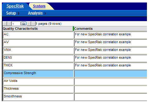
Figure 65. Screenshot. Quality characteristics for selection in SPECRISK.
Pay Equation Setup
The next step is to make sure the necessary pay equations are included as part of the setup procedure. The highlighted line in figure 66 shows the entry of the new pay equation for this analysis. Since the same pay equation is used for both quality characteristics, only a single entry is required. In figure 66, the user has described the pay equation in the comments section for convenient future reference.

Figure 66. Screenshot. Pay equation designation.
The actual entry of the mathematical properties of the equation is accomplished with the aid of the pay equation wizard (see figure 67). The user enters the information that the pay equation yields as follows: the constant value of PA = -0.24 from PWL = 0 to PWL = 50 and the equation PA = -0.54 + 0.006 PWL from PWL = 50 to PWL = 100.

Figure 67. Screenshot. Pay equation wizard for specification 3.
Once the pay equation has been entered, a graph can be used to check that the equation will function as intended. Figure 68 shows that the compound equation has been designed to assign a PA of -0.24 from PWL = 0 to PWL = 50 and applies the equation PA = -0.54 + 0.006 from PWL = 50 to PWL = 100.
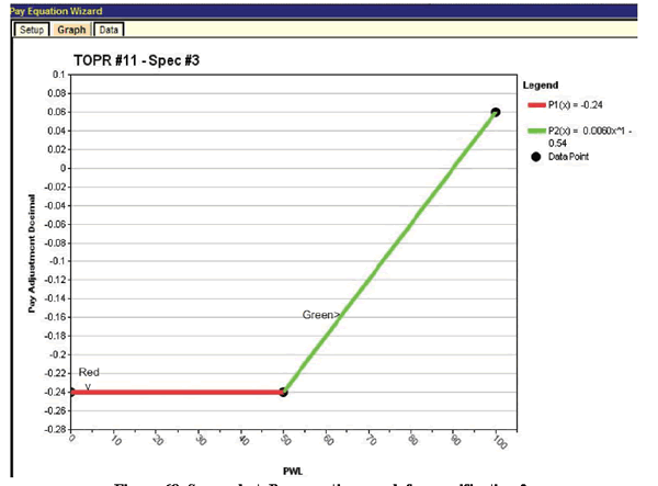
Figure 68. Screenshot. Pay equation graph for specification 3.
Entering Data into Simulation Profile
For this specification, it was necessary to create a new profile for analysis as described for specification 1. Figure 69 shows the newly created profile for specification 3.

Figure 69. Screenshot. Part of SPECRISK profile screen for specification 3.
In the fourth column in figure 69, "Pay Adjustment Decimal" was selected as the appropriate form for the pay equation. In the next column, 1,000 was entered as the number of iterations of the simulation process. The cropped screenshot in figure 69 shows only a few of the several output features that can be selected. Unless the analyst knows for certain that they are not needed, it is advisable to check all of the available boxes because of the useful information they can provide.
The next several steps involve entering the basic specification 3 information from the "Acceptance Procedure Synopsis" section. To begin, the user clicks on "Quality Characteristic Data Entry" (see figure 70). Some of the entries are typed in directly, while others are selected after clicking on the down arrows that appear in some cells.

Figure 70. Screenshot. Specification 3 quality characteristic data entry.
As shown in figure 70, after creating two blank rows, the user has clicked the down arrows in the second column and selected "Compressive Strength" and "Thickness." The appropriate pay equations are selected in a similar manner in the third column, followed by the selection of "1-sided" as the limit type in the fourth column. Next, the sample size of 5 and the AQL of PWL = 90 are entered for both quality characteristics. The "Acceptance Procedure Synopsis" section notes that whenever the sample average falls below the lower specification limit, the corresponding PWL value is not calculated and is set to a minimum value of PWL = 50. Therefore, "50" has been entered in the RQL cell for both quality characteristics.
Whereas the SHA does not calculate the actual PWL value when AVG is less than LSL but sets PWL = 50 and applies the minimum pay level, the SPECRISK procedure does calculate PWL and, if it is 50 or less, applies the minimum PF prescribed by the pay equation, as shown in figure 68. The end result is the same, but because of this difference, the SPECRISK analysis gathers additional data that can be displayed and may be of interest. For example, SPECRISK can determine how often this action occurs at different levels of actual production quality.
The rest of the input proceeds in much the same manner. The quality characteristics are not correlated for this application, so this input step can be bypassed. An additional column at the right of figure 70 allows a checkbox for "Retest" to be clicked. Retesting does not apply for this application nor do additional selections not shown in this figure.
As previously noted, the appropriate weighting factor is 0.5 for both of the quality characteristics. This information is entered by clicking on "Pay Relationship Data Entry," selecting "Weighted Average" as the type of pay relationship, and then entering the appropriate weights in the right column in figure 71.
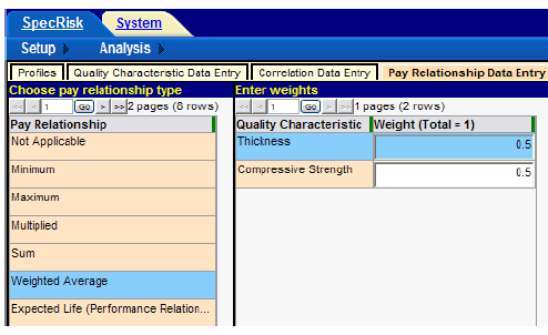
Figure 71. Screenshot. Entry of pay weighting factors for specification 3.
The next tab, "OC Curves Data Entry," allows the user to enter pay levels from which a series of graphed OC curves will be produced, showing the probability of receiving these pay level (or higher) at any level of true population quality. The pay schedule for this application is in units of PA in decimal form. An appropriate series of pay levels has been entered in figure 72.
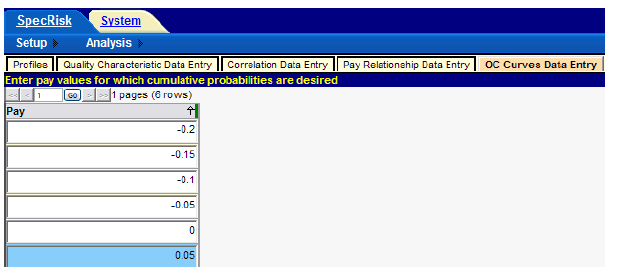
Figure 72. Screenshot. Entry of pay levels for specification 3 OC curve analysis.
Preliminary Analyses
Following the input of essential entries for analysis of the specification, it is customary to perform a preliminary analysis by entering a few key quality level combinations in the “Analyze Selected” table, as shown in figure 73. This early analysis can provide almost immediate results at quality levels of particular importance and may allow the user to spot obvious input errors.

Figure 73. Screenshot. Preliminary run at key quality level combinations.
For example, the highlighted line in figure 73 shows that at the AQL for which both quality characteristics are at PWL = 90, the expected (i.e., long-term average) PA of 0.0002 is almost exactly at the desired value of 0.0. This indicates that a contractor who consistently performs at the AQL for both quality characteristics will receive essentially no PA in the long run and thus will be paid 100 percent for producing precisely the level of quality specified as acceptable, which is desired. There is a 5 percent chance that the contractor would receive a reduction of -0.067 when actually at the AQL. This is an indication of the influence of sample size on the acceptance procedure.
In the next two rows, one quality characteristic is held at the AQL of PWL = 90, while the other is set at PWL = 50, which is a deficient level of quality. Since the same pay equation is applied to both quality characteristics, and they both have equal weights of 0.50, the expectation that both of these combinations should produce about the same level of PA is confirmed in figure 73. The SPECRISK analysis indicates that the expected PA in both cases is close to -0.099, a pay reduction of approximately 10 percent. The SHA must decide if this is a sufficient level of pay reduction for this degree of deficient quality.
The last two rows in figure 73 show PWL combinations of 50/50 and 0/0 produce expected PAs of -0.19 and -0.24, respectively, which confirms that the analysis procedure is performing as expected. When both quality characteristics are exactly at PWL = 50, approximately half of them will test out as PWL < 50 and then be set at PWL = 50, as this procedure prescribes. The other half will test out at PWL > 50 and be recorded as they actually occur. Consequently, the longterm average will be something above PWL = 50, and the simulation analysis has determined that this equates to an expected PA of approximately -0.19.
When both quality characteristics are essentially at PWL = 0, virtually all estimates will also be at PWL = 0 and all will be set at PWL = 50. The pay equation in figure 64 shows that this corresponds to an expected PA of -0.24, as confirmed in the last row in figure 73.
Full Analysis
For many SHAs, the preliminary analysis may be sufficient to confirm that the acceptance procedure is working satisfactorily or to demonstrate that modifications need to be made. For those desiring more detailed information, a full analysis can be run. Several output graphs generated from the full analysis of specification 3 are included in this section.
Whereas the preliminary analysis in figure 73 provided the expected PA levels at certain important combinations of quality levels, the EP graphs in figure 74 through figure 76 provide information over the entire range of possible quality levels. For research or troubleshooting purposes, the individual characteristic graphs shown in figure 74 and figure 75 can be useful, but the composite results in figure 76 represent the overall payment to the contractor and are likely to be of greatest interest.
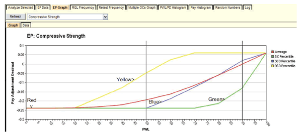
Figure 74. Screenshot. EP graph for compressive strength.
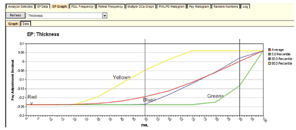
Figure 75. Screenshot. EP graph for thickness.
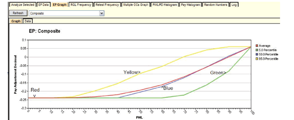
Figure 76. Screenshot. EP graph for composite results.
In all three figures, the red line represents the average (expected) payment levels throughout the entire range of quality from PWL = 0 to PWL = 100. The other lines represent selected percentile levels that provide a visual indication of how variable individual lot pay levels may be about the average.
As previously noted, the same pay equation is applied to both quality characteristics, and they have equal weights of 0.50. Thus, it is expected that the EP graphs for both compressive strength and thickness should be nearly identical, as shown in figure 74 and figure 75.
In order to be able to plot figure 76, it is necessary to hold all quality characteristics simultaneously at the PWL values shown on the x-axis. This allows the graph to be plotted in two dimensions for multiple quality characteristics and provides a reasonably good picture of how the acceptance procedure will perform. However, SPECRISK does compute the data needed for a more complete analysis that allows all possible combinations of quality levels. These analyses can be accessed by clicking on the "EP Data" tab.
Two interesting observations can be made from figure 76. First, as seen in the individual characteristic graphs, the red line (average PA) goes almost exactly through PA = 0 at the AQL of PWL = 90, as desired. Second, because figure 76 represents the weighted average of the two individual pay results, the percentile lines are generally less dispersed than they are for the individual quality characteristics. This is roughly analogous to the statistical effect of the standard error of the mean.
Another display of interest is the multiple OCs graph shown in figure 77. Like figure 76, the graph is constructed with all quality characteristics held simultaneously at the PWL values on the x-axis.
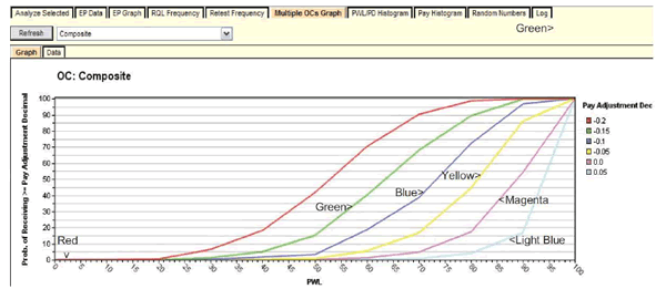
Figure 77. Screenshot. Multiple OCs graph for specification 3.
In this case, the curve of primary interest is the purple line, which represents the probability of achieving an average PA factor of 0.0 or higher (i.e., a PF of 100 percent or more). Figure 77 shows that when the contractor performs consistently at the AQL of PWL = 90, there is about a 0.55 probability of achieving a PA of 0.0 or higher. In other words, approximately half of the PAs will be above 0.0 (some degree of incentive), and half will be below (some degree of reduction) such that the long-term average will be almost exactly 0.0 (100 percent payment), as desired. This is confirmed by the red curve in figure 76.
Both the composite EP and multiple OCs graph can be useful to the SHA and the contractor. For the conservative contractor who wants to assure a greater frequency of PAs of 0.0 or an incentive, figure 77 shows that a consistent production level of PWL = 95 would produce a probability of about 0.78 of receiving some degree of incentive payment. Figure 76 shows that the average positive incentive payment would be about 0.03.
A final graph of interest for this analysis displays the frequency with which an RQL clause (and possible remove-and-replace option) would be triggered. Since this specification does not define the RQL in the manner for which the SPECRISK software was designed (level of PWL or PD), the value of PWL = 50 was entered as the RQL value because this is the point below which the agency chooses to set the measured value to a constant level of PWL = 50. Figure 78 shows the expected frequency of occurrence of this action for compressive strength, and since the two quality characteristics are treated identically, this figure would also apply to thickness.
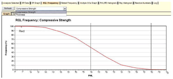
Figure 78. Screenshot. Frequency of estimates of PWL ≤ 50 at various PWL levels.
As shown in figure 78, at a consistent production level of PWL = 50, action would be expected to occur about 50 percent of the time. This approximate result is expected because PWL is an unbiased statistical estimator. What could not be so easily determined is that, when the production is consistently controlled at PWL = 65, for example, action will still occur about 20 percent of the time. Similarly, at a very poor production level of PWL = 35, the material will test out as PWL = 50 or higher about 20 percent of the time due to inherent statistical variability at this sample size (n = 5). Thus, this graph can provide the agency with information needed to decide if some sort of retest provision or other adjustment might be desirable, depending on the actual consequences of potential errors of this magnitude. The curve also shows that when at the AQL of PWL = 90, there is little or no chance that the estimated PWL will result in a minimum payment. This will ordinarily be the case at the AQL but warrants checking when the sample sizes are relatively small.
SPECRISK does not provide this capability directly, but an additional inference can be drawn from figure 78. Since the OC curve applies to both compressive strength and thickness, and the probability of triggering the setting of PWL = 50 when the true production level is exactly PWL = 50 is almost exactly 0.50, the probability of not triggering this action is also 0.50 for both compressive strength and thickness. Therefore, when the production is controlled at PWL = 50, the combined probability of not triggering this action for both quality characteristics is 0.50 × 0.50 = 0.25, and the probability of triggering it for at least one of them is 1.00 – 0.25 = 0.75. By trial and error, it can be found that when production is controlled at PWL = 61, the probability of either compressive strength or thickness triggering this action is about 0.50. This can often be useful information, depending on the consequences of this level of quality, and the severity of the PA or required remedial action.
Analysis Summary and Conclusions
The following are the key components and conclusions of this analysis:
SPECIFICATION 4
Introduction
Under specification 4, the SHA accepts PCC pavement based on measuring compressive strength, thickness, and smoothness. This analysis considers compressive strength and thickness and is limited to class 1 PCC. The analysis for class 2 PCC would be conducted in the same manner as class 1. Smoothness is controlled by a shutdown procedure for any section of pavement exceeding 7 inches/mi using the agencies test procedure. This requirement is not conducive to QA analysis and was not conducted.
Since this SHA uses an average with no measure of variability as the quality measure, the analysis is much more involved than the previous three specifications, which used PWL.
Compressive Strength Acceptance
The pavement is subdivided into separate concrete lots of approximately 5,333 yd2 placed continuously (e.g., 2,000 ft by 24 ft). Cylinders are then tested for compressive strength.
Acceptance based on 24-h compressive strength is as follows:
If the average 28-day compressive strength of the lot does not meet the lower acceptance limit for a 0.70 PF, the agency either orders removal of the concrete in the lot, or applies a PF of 0.50 for the lot.
The unit price of concrete pavement will be reduced for areas represented by each lot that does not meet the specified compressive strength at 28 days, according to table 3.
| PF | Average Compressive Strength | |
|---|---|---|
| Class 1 | Class 2 | |
| 1.00 | ≥ 3,000 psi + 0.18R | ≥ 3,500 psi + 0.21R |
| 0.95 | ≥ 3,000 psi – 0.07R | ≥ 3,500 psi – 0.07R |
| 0.70 | ≥ 3,000 psi – 0.30R | ≥ 3,500 psi – 0.30R |
R = Sample range.
Analysis of Compressive Strength Acceptance Plan
Since it would require a detailed knowledge of what the SHA believed to be the relationship between 24-h and 28-day concrete compressive strength, it is not possible to analyze the effect that the 24-h strength requirement has on acceptance and payment determination for PCC. It would also be necessary to know what relationship actually exists for concrete mixed and placed on the SHA’s projects and the mean and standard deviation for the population of 24-h strengths. This relationship is made more complex by the fact that it would need to be correlated to the 28 day strengths, which are also variable. Without extensive SHA data for many corresponding 24-h and 28-day test results, it is not possible to conduct any sort of valid analysis of this acceptance provision. As a result, the following analyses consider only the 28-day compressive strength requirements.
Determining the AQL
To analyze the risks associated with an acceptance plan, it is necessary to know what the SHA considers the AQL. It is generally accepted that the contractor should receive an average payment of 100 percent for producing an AQL population. Since the AQL that the SHA used is not known (or even whether or not the SHA established an AQL population), an assumed AQL must be established based on the acceptance plan requirements.
The AQL can be approximated based on the requirement for a PF of 1.00. That is, the AQL can be defined as a population that meets the requirement of 3,000 psi + 0.18R. Since this payment relationship includes values for both the mean, as measured by the sample average, and the variability, as measured by the sample range, R, there are many populations that meet the AQL requirement. Using this assumption, the AQL population for class 1 PCC can then be defined as shown in figure 79.
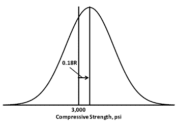
Figure 79. Graph. Assumed AQL population for class 1 PCC compressive strength.
One issue with the AQL in figure 79 is that it is defined in terms of the range, which is not a useful measure when defining a normal population as is usually assumed for construction materials. However, there is a statistical relationship between the mean range, R, for data from a normal distribution and σ, the standard deviation of that distribution. This relationship depends only on the sample size, n. The mean of R is R = d2σ, where the value of d2 is also a function of n. The d2 values for various sample sizes are shown in table 4.
| Sample Size, n | d2, where R= d2σ |
|---|---|
| 6 | 2.534 |
| 7 | 2.704 |
| 8 | 2.847 |
| 9 | 2.970 |
| 10 | 3.078 |
The value d2σ can therefore be substituted for R in the AQL shown in figure 79. However, table 4 shows a potential problem with the acceptance plan. The relationship between sample ranges and the population’s standard deviation varies with the sample size. However, while the acceptance plan indicates that at least six cylinder should be tested (based on American Association of State Highway and Transportation Officials (AASHTO) T-22 and ASTM C-192), it includes only a single threshold limit for each PF.[4,5] Since the limits do not change with sample size, this creates a situation where the AQL in figure 79 is different for each sample size. Ideally, the AQL is a constant value defined by the highway agency based on engineering considerations and experience.
For example, the means of the AQL population for n = 6 and n = 10 are calculated in figure 80 and figure 81.
![]()
Figure 80. Equation. Required offset of the mean of a population based on a sample size of n = 6.
![]()
Figure 81. Equation. Required offset of the mean of a population based on a sample size of n = 10.
Figure 82 shows the probability density functions (PDFs) for the AQL populations for sample sizes n = 6 and n = 10. The two PDFs can be plotted together since the population mean, μ, is represented in terms of the number of population standard deviations from the lower specification limit, LSL = 3,000. That is, the mean is plotted as ( μ – 3000)/ σ.
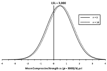
Figure 82. Graph. Assumed AQL populations for class 1 PCC compressive strength.
Since many different combinations of population means and standard deviations meet the AQL of the acceptance plan, it is related in concept to the PWL approach. Using a table of the standard normal distribution or a computer software program, such as Microsoft Excel® or Minitab®, the PWL value can be calculated for each of the AQL populations shown in figure 82. These PWL values are 67.6 for n = 6 and 71.0 for n = 10. As discussed later in this chapter, the use of the sample PWL rather than the sample mean and range eliminates the problem of different AQLs for different sample sizes.
Determining Expected Payment Curves
For many reasons, including the use of the range rather than standard deviation, the differing AQL populations for different samples sizes, and the literally infinite combination of population means and standard deviations that can be considered AQL populations, the best way to analyze the acceptance plan is by using computer simulation. In this case, Minitab® statistical software was used to generate samples of varying sizes from different populations. Although a larger number of iterations would be preferable for a detailed analysis, samples for 10,000 lots were simulated for illustration purposes. For each lot, the sample mean and range were calculated, and these values were used with table 3 to determine the PF for the lot. The 10,000 lot payment factors were then averaged to determine the expected payment for each sample size and level of quality simulated. In the simulations, lots that did not meet the requirements for a 0.70 PF were assigned a PF of 0.50.
The results of the simulations were then plotted to develop the EP curve in figure 83. This curve is for samples of size n = 6. Since the level of quality is represented in terms of the number of population standard deviations that the population mean is above the lower specification limit of 3,000 psi, this single curve can be used to determine the EP value for any population.
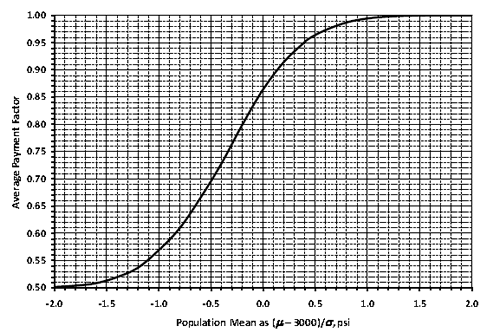
Figure 83. Graph. EP curve for class 1 PCC for n = 6.
For example, if the contractor produced a population with μ = 3,200 psi and σ = 500 psi, this would correspond to a value of (3,200 – 3,000)/500 = 0.4 on the x-axis in figure 83. As shown in figure 84, this corresponds to an average PF, or expected payment, of approximately 0.95. If the contractor produces this same population numerous times, it would be expected that the individual lot PF would average about 0.95. This same expected payment value would be obtained if the contractor produced a population with μ = 3,400 psi and σ = 1,000 psi, since it would correspond to the same value of (3,400 – 3,000)/1,000 = 0.4.
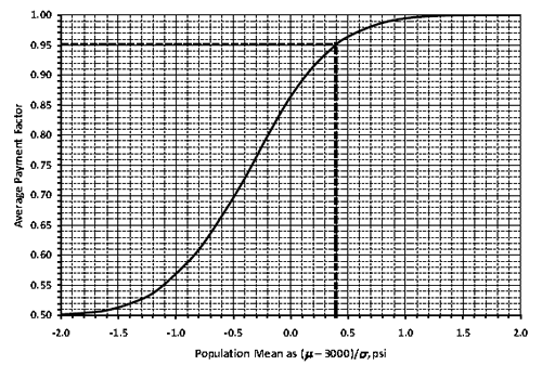
Figure 84. Graph. EP curve for population with (μ – 3,000)/ σ = 0.4 and n = 6.
Figure 80 shows that the population mean for an AQL population for n = 6 would be 0.456 above the lower specification limit of 3,000 psi. From either figure 83 or figure 84, the expected payment value can be calculated for this AQL population and would be approximately 0.96. This illustrates what might be called the "payment risk" to the contractor. If a contractor produces an AQL population, the PF should be 1.00. However, a contractor that consistently produces the AQL population will instead average only 0.96 for the PF.
This payment risk is at least partially, and perhaps totally, due to the fact that the acceptance plan does not provide an incentive for material that exceeds the AQL quality. Due to the random nature of the sampling process, there will be times when material that is precisely at the AQL but will have a sample result that indicates a reduced PF should be applied. However, since there is no incentive provision, the times when the sample result indicates quality in excess of the AQL this will result in a PF of 1.0. Therefore, it will not be possible for AQL material to receive an average PF of 1.0.
To receive an expected payment of 1.0, the contractor must produce a population with a mean that is at least 1.4 standard deviations above 3,000 psi (see figure 83). Using the previous example with σ = 500, this corresponds to a population mean of 3,000 + (1.4 × 500) = 3,700 psi, which is considerably higher than the AQL mean of 3,000 + (0.456 × 500) = 3,228 psi. This could be interpreted to mean that the contractor must produce quality much greater than the AQL to be able to average full payment. Or, these results might be interpreted to redefine the AQL to be a population for which the mean is at least 1.4 standard deviations above the lower specification limit of 3,000 psi. However, the specification does not clearly communicate the definition of the AQL.
Simulations were conducted on sample sizes of n = 6, 8, and 10 to evaluate the effect that sample size has on the expect payment values. Figure 85 presents the EP curves for the case of sample sizes of n = 6 and 10. The sample size of n = 8 was between the two curves and was not plotted so that the two curves were easier to see. The larger sample size results in slightly larger expect payment values. For the previous example, where ( μ =3000)/σ = 0.4 for n = 6, the expected payment is approximately 0.95. Figure 85 shows that the same population has an expected payment of approximately 0.96 when n =10.
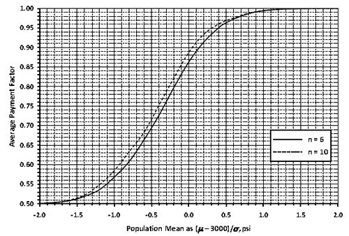
Figure 85. Graph. EP curves for class 1 PCC for n = 6 and n = 10.
Determining OC Curves
The EP curve shows the long-term average payment for any given quality level. However, it does not provide any information regarding the variability about this average of the individual lot PFs. One way that this variability might be considered is to look at the standard deviation value for the 10,000 lot simulations that were used to determine the expected payment values. The standard deviations for selected quality levels, in terms of ( μ – 3,000)/σ , are plotted in figure 86 for sample sizes of n = 6 and n = 10. The standard deviation values are consistently lower for the larger sample size. In general, this means that larger samples tend to produce better estimates of the population parameters.
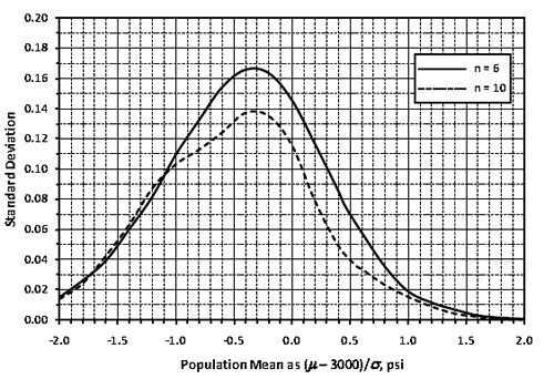
Figure 86. Graph. Standard deviations of PFs for class 1 PCC for n = 6 and n = 10.
Figure 86 provides information on variability, but it does not provide any information regarding the likelihood of receiving a specific PF. Therefore, another step necessary to fully evaluate the risks is to plot OC curves associated with the probabilities of receiving various PFs. Figure 87 shows OC curves for the probability of receiving greater than or equal to each of the possible PFs when using a sample size of n = 6.
Figure 87. Graph. OC curves for class 1 PCC compressive strength for n = 6.
While the EP curve in figure 83 shows that the average long-term payment at the AQL, (μ – 3,000)/ σ = 0.456) is approximately 0.96, the OC curves in figure 87 show that the probability is only about 0.5 that any individual lot of AQL material will receive a PF of 1.0. Therefore, there is also about a 0.5 probability that a contractor would receive less than full payment for a lot that was of AQL quality. Similarly, figure 88 shows the OC curves for a sample size of n =10. Again, the probability is only about 0.5 that any individual lot of AQL material will receive a PF of 1.0.
Figure 88. Graph. EP curves for class 1 PCC compressive strength for n = 10.
Although figure 87 and figure 88 show the same probabilities at the AQL for n = 6 and n = 10, the AQL differed for each sample size. For a given population, the probabilities of receiving various PFs will be different for different sample sizes. This is because the AQL varied with sample size, but the acceptance limit was constant for all sample sizes. Figure 89 illustrates these differences in payment probabilities. For example, for a population with ( μ – 3,000)/ σ = 0.5, the probability of receiving a PF of 1.0 is approximately 0.55 for n = 6 but is only about 0.45 for n = 10. This may seem surprising since figure 85 shows that for the same population, the expected payment is greater for n = 10 than it is for n = 6. However, this is the case because figure 89 also shows that for n = 6, this same population has about a 0.05 probability of receiving a payment factor of 0.7 or lower (1.0 – 0.95 in figure 89), whereas for n = 10, this same probability is 0.01 or less.
Figure 89. Graph. OC curves for class 1 PCC compressive strength for n = 6 and n = 10.
Recommendations for Improving the Strength Specification
Some of the issues with this specification, along with some recommended changes to the acceptance plan, are presented in the following sections.
Acceptance Based on 24-h Compressive Strength
A conscientious contractor should easily meet the minimum early acceptance strength requirement by increasing the cement content above that used in the design. If the average of the three lot acceptance tests equal or exceed the minimum early strength, the lot will be accepted at the full contract price. Thus, acceptance is based on a sample size of n = 3, a lower sample size than that used in the 28-day acceptance. Small sample sizes such as this may not provide sufficient discriminatory power to clearly distinguish between satisfactory and unsatisfactory material. In other words, based on the information available at 24 h, it is not possible to determine how frequently this requirement might accept material that is truly defective or reject material that is truly satisfactory. It further insures a PF of 1.00 without additional testing. So, the contractor knows immediately what the PF will be. As stated above, the risks cannot be analyzed without making many assumptions, but based on the sample size alone, the risks are certainly higher than those in the 28-day requirement.
Discrete Payment Schedule
Specification 4 uses a discrete, or stepped, payment schedule where small differences in quality can result in large differences in the payment factor received. When the true quality level of the work happens to lie close to a boundary in the stepped payment schedule, the quality estimate obtained for an individual lot may fall on either side of the boundary due primarily to chance. Depending upon which side of the boundary the estimate falls, there may be a substantial difference in payment level, which may lead to disputes over measurement precision, round-off rules, and so forth. This problem can be avoided with a continuous payment schedule that provides a smooth progression of payment as the quality measure varies.
For example, suppose that a contractor is operating under the payment schedule in table 3. Furthermore, suppose that the following compressive strength test results are obtained from a lot: 2,790, 3,140, 2,945, 3,850, 3,105, and 3,310 psi. The sample mean is 3,190 psi and the sample range is 1,060 psi. From table 3, the threshold for a PF of 1.0 is 3,000 + 0.18R, or 3,000 + (0.18 × 1,060) = 3,190.8 psi. Since 3,190 < 3,190.8, the PF would be 0.95. If the last test result had instead been 3,316 psi, (an increase of only 6 psi) then the mean would be 3,191 psi, which exceeds 3,190.8 psi and puts the PF at 1.0. This is a fairly large payment reduction (5 percent) for essentially no difference in the measured quality. The difference would obviously be even more significant at the boundary between 0.95 and 0.70 PFs.
Use of the Sample Range
The sample range is not the best measure to use for variability; the sample standard deviation is a better choice. When statistical specifications were first developed, the range was sometimes used due to its simplicity of calculation. However, with the availability of computers, there is no reason not to use the standard deviation instead of the range.
The way that the range is used creates several other issues that have been discussed. First, the use of the range with a single set of PF limits creates, in essence, a different AQL population for each sample size. The AQL should be unique and established as an engineering decision prior to developing the acceptance plan.
The different AQL requirements create the situation shown in figure 85, where the expected payment for a population is different for different sample sizes. It is important for the contractor to be able to determine from the specification exactly what is required to receive full payment. As written, unless the contractor knows in advance the exact sample size, there is no way to know with certainty the requirement for a PF of 1.0.
Use of PWL Approach
The use of PWL as the quality measure is a much better and more efficient approach for incorporating both the sample mean and sample standard deviation into the PF determination. The PWL approach incorporates the sample size into the PWL determination, which eliminates the problem that exists where there are different expected payment values for different sample sizes.
The PWL approach is statistically valid, is endorsed by FHWA, has been in use for decades, and has been adopted by numerous SHAs. The existing specification could be easily adapted to the PWL. As previously discussed, the PWL for the AQL populations vary around a value of approximately 70. This could be used as the PWL value required for full payment and the new PWL specification would be related to the existing specification quality. However, a PWL of 90 is a much more common value for AQL, and a corresponding 1.0 PF. It would probably be preferable to modify the AQL and payment relationships in the specification to be more in line with a value of 90 PWL.
Lack of an Incentive Provision
This specification does not include an incentive provision that allows PFs greater than 1.0. There are several arguments in favor of allowing an incentive payment for quality that exceeds the specified quality level. The most important is a matter of fairness.
Due the random nature of the sampling process, there will be times that material at the AQL will have a sample result that indicates a reduced PF should be applied. However, if there is no incentive provision, the times when the sample result indicates quality in excess of the AQL will result in a PF of 1.0. Therefore, it will not be possible for AQL material to receive an average PF of 1.0. This is clearly illustrated in the EP curves in figure 85.
The solution is simple; a relatively small incentive for work exceeding the specified AQL will correct this situation. In all cases, the EP and OC curves should be constructed to confirm that the acceptance procedure is working as desired and, in particular, that the average PF at the AQL is 1.0.
Thickness Acceptance
This analysis is also limited to class 1 PCC. The analysis for class 2 PCC would be conducted in the same manner.
Pavement thickness is determined using average core measurements. One core is taken for each 2,000 yd2 of pavement in each unit. If the core measurement is ≤ 0.2 inches from the plan thickness, full payment is made. If the core measurement is deficient > 0.2 inch and not more than 1 inch from the plan thickness, two additional cores are secured from the unit and used to determine the average thickness. A random selection process determines where to secure additional cores. However, cores are not secured within 50 ft of other thickness measurement cores. If average thickness is deficient by more than 0.2 inches, the payment factor is determined from table 5.
| Deficiency in Thickness (Inches) | Proportional Part of Contract Price Allowed (Percent) |
|---|---|
| 0.0–0.2 | 100 |
| 0.21–0.25 | 95 |
| 0.26–0.30 | 91 |
| 0.31–0.40 | 86 |
| 0.41–0.50 | 80 |
| 0.51–0.75 | 70 |
| 0.76–1.00 | 60 |
When the thickness of pavement is deficient by more than 1 inch and the engineer determines that the deficient area should not be removed or replaced, 50 percent of the contract unit price will be paid.
Analysis of Thickness Acceptance Plan
Determining the AQL
To analyze the risks associated with an acceptance plan, it is necessary to know what the SHA considers the AQL. Since the AQL that the SHA used for this specification is not known (or even whether or not the SHA established an AQL population), an assumed AQL based on the acceptance plan requirements can be established.
Since it is generally accepted that AQL material should receive full payment, the AQL can be approximated based on the requirement for a 100 percent PF. That is, the AQL can be defined as a population that meets the requirement that the sample average is ≤ 0.2 inches below the plan thickness. This, however, is not sufficient to determine the AQL population since there could be many populations for which this requirement could apply. To be able to determine the AQL population it would be necessary to know two of the following items that the SHA used when developing the acceptance plan: the population mean, the population standard deviation, and the seller’s risk, ∝. Figure 90 illustrates how these values interact to define the AQL population.
Figure 90. Graph. Defining the AQL for thickness.
Without knowing what mean, standard deviation, or seller’s risk the SHA decided on, the only way to analyze this specification is by means of EP and OC curves. The acceptance procedure in this specification is based on the sample mean of samples of size n =1 or n =3, but does not include any measure of variability in the acceptance decision. This approach is sometimes called a "variability known" specification. With this approach, since the variability is not measured, the SHA is implicitly assuming that the contractor produces a population with a standard deviation equal to or less than the one used by the SHA when the specification limits were developed.
The best way to evaluate this specification is to develop EP and OC curves for populations with varying means but with a constant standard deviation. In this way, a set of EP and OC curves can be developed for each standard deviation value to be considered. This is the approach used in the analyses that follow.
Acceptance on a Single Core
There are two ways in which a contractor can receive 100 percent payment for thickness. First, a single core is tested, and the contractor receives 100 percent payment if the core thickness is ≤ 0.2 inches below the plan (or target) thickness. This provision can be evaluated using analytical procedures. If a population mean and standard deviation are selected, the probability of meeting this provision can be calculated from the area under a normal distribution curve. For example, suppose the contractor produces a population with mean thickness equal to the target thickness and a standard deviation of 0.25 inches. The probability that the contractor will receive 100 percent payment based on a single core is the shaded region shown in figure 91. It is assumed that there is no upper limit on thickness, since the specification did not mention one.
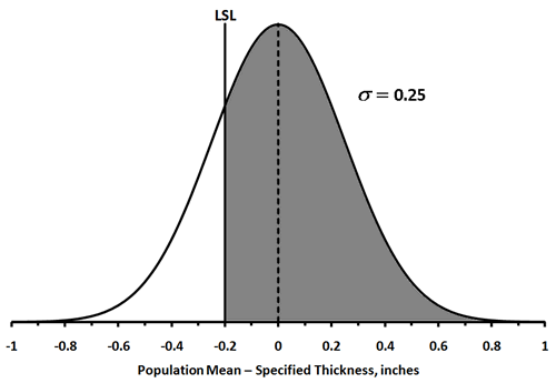
Figure 91. Graph. Probability of receiving 100 percent payment for a population with mean equal to the target and σ = 0.25 inches.
The probability of accepting on a single core from the population shown in figure 91 can be calculated using a table of the standard normal distribution or with statistical software. The Z-statistic to use with a standard normal distribution is calculated in figure 92.
![]()
Figure 92. Equation. Z statistic.
Using a standard normal table or software, this probability is calculated to be 0.788. Similar probabilities can be calculated for various population means with σ = 0.25 inches to develop the curve shown in figure 93. This curve represents the OC curve associated with the probability of receiving full payment based on the first core sampled.
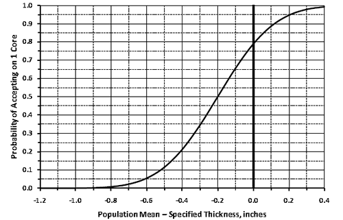
Figure 93. Graph. OC curve for probability of full payment based on a single core if σ = 0.25 inches.
Calculations similar to those used to develop figure 91 and figure 93 can be conducted to develop similar curves for any standard deviation selected. For example, figure 94 shows the probability that the contractor will receive 100 percent payment based on a single core for a population with mean thickness equal to the target thickness and a standard deviation of σ = 0.50 inches.
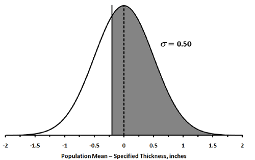
Figure 94. Graph. Probability of 100 percent payment for a population with mean equal to the target and σ = 0.50 inches.
Figure 95 shows the OC curves for the probability of receiving full payment based on a single core for populations with σ = 0.25 and 0.50 inches. The curves in figure 95 are quite different for the two population standard deviations. These differences are apparent when the populations are shown on the same plot. For example, figure 96 shows the σ = 0.25- and 0.50-inch populations plotted with each having a mean equal to the target value. It is obvious that the population with the smaller standard deviation has a greater percentage above the specification limit of 0.2 inches below the target value.
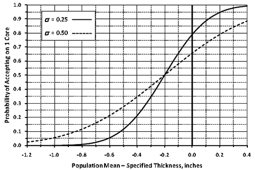
Figure 95. Graph. OC curves for probability of full payment based on a single core.
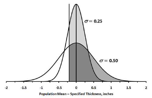
Figure 96. Graph. Comparison of probabilities of 100 percent payment for populations with mean equal to the target.
If the first core is deficient in thickness by > 0.2 inches, two additional cores are taken, and payment is based on the average deficiency of the three cores. When acceptance is based on the average of several results the probability of acceptance normally can be calculated in a similar fashion to the case above for a single core. The calculations rely on the fact that the standard deviation of the distribution of sample means, σ x , equals the population standard deviation divided by the square root of the sample size, σ x = σ /√n.
However, this assumes that the three cores are sampled at random from the population. For this specification, the cores are not taken at random since the second two cores are not sampled unless the first core is deficient in thickness by > 0.2 inches. Therefore, the sample is biased since at least one of the three cores must be more than 0.2 inches below the target. As a result, the probability of receiving full payment based on the average of three cores will be less than that calculated for a true random sample. The best way to calculate the probability of receiving full payment is by using computer simulation. The methodology for doing this is presented and discussed in the section on developing OC curves.
Determining EP Curves
As explained in the previous section, the best way to analyze this acceptance plan is by using computer simulation. In this case, Microsoft Excel® was used to generate samples of size n = 3 from various populations. Although a larger number of iterations would be preferable for a detailed analysis, samples of 10,000 lots were simulated for illustration purposes. For each lot, if the first core result was ≤ 0.2 inches below the target thickness, the lot was assigned a payment factor of 100 percent. If the core was deficient in thickness by > 0.2 inches, then the three core thicknesses were averaged, and payment for the lot was determined by the schedule in table 5.
The 10,000 lot payment factors were then averaged to determine the expected payment for each population mean and standard deviation simulated. In the simulations, the population standard deviation was held constant while the population mean was varied to represent different levels of quality. In the simulations, lots that did not meet the requirements for a 60 percent PF were assigned a PF of 50 percent. Other assumptions could have been made. For example, a payment factor of 0 percent could have been used to correspond to a remove-and-replace requirement.
For each standard deviation, the results of the simulations were then plotted to develop EP curves such as the one shown in figure 97 for σ = 0.25 inches. Since the level of quality is represented in terms of the distance in inches that the population mean is above or below the specified target value, this single curve can be used to determine the expected payment value for any target thickness. Figure 97 shows that if the contractor produces a population with mean equal to the target thickness, the expected payment value will be nearly 100 percent (the actual simulated value was 99.6 percent).
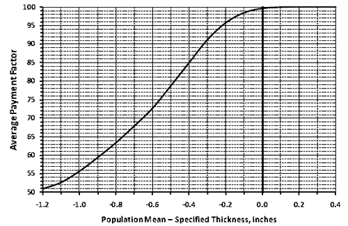
Figure 97. Graph. EP curve for PCC thickness for σ = 0.25 inches.
Simulations were conducted for σ = 0.25, 0.30, and 0.50 inches to evaluate the effect that population standard deviation has on the expected payment values. Figure 98 presents the EP curves for the three standard deviations simulated. The larger standard deviation resulted in lower expected payment values near the target. For σ = 0.30 inches, the differences are not large, with the expected payment at the target thickness still over 99 percent. However, for σ = 0.50 inches, the expected payment drops to just over 97 percent at the target thickness.
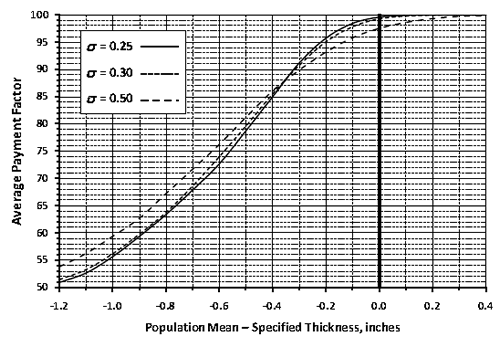
Figure 98. Graph. EP curves for PCC thickness for various population standard deviations.
Determining OC Curves
The EP curve in figure 97 shows the long-term average payment for any given quality level when σ = 0.25 inches. However, it does not provide any information regarding the variability about this average of the individual lot PFs. One way that this variability might be considered is to look at the standard deviation value for the 10,000 lot simulations that were used to determine the expected payment values. The standard deviations for selected quality levels, in terms of population mean minus target thickness, are plotted in figure 99 for σ = 0.25, 0.30, and 0.50 inches. The standard deviation of individual PF values is consistently lower for the smaller population standard deviations.
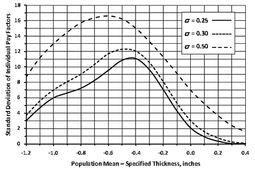
Figure 99. Graph. Standard deviations of PFs for various population standard deviations.
Figure 99 provides information on variability, but it does not provide any information regarding the likelihood of receiving a specific PF. Therefore, to fully evaluate the risks for this specification, it is necessary to plot OC curves associated with the probabilities of receiving various PFs. Figure 100 shows OC curves for the probability of receiving greater than or equal to each of the possible PFs for this specification when using σ = 0.25 inches.
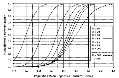
Figure 100. Graph. OC curves for PCC thickness for populations with = 0.25 inches.
While the EP curve in figure 97 shows that the average long-term payment at the specified target thickness is approximately 99.6 percent, the OC curves in figure 100 show that the probability is only about 95 percent that any individual lot will receive a PF of 100 percent. The dashed line in figure 100 is the probability that full payment will be received based on the thickness of the first core tested. This line, which is based on the simulation results, corresponds to the similar line in figure 93 that was developed using analytical techniques. The two lines are quite close, with small differences due to the relatively small number of lots that were simulated.
To demonstrate the effect that population standard deviation has on the PF received, figure 101 shows the OC curves for populations with σ = 0.50 inches. Comparing figure 100 and figure 101 shows the differences in payment probabilities for the different population standard deviations. The populations with the larger standard deviation have lower probabilities of receiving each PF for populations with means near the target thickness, and higher probabilities of receiving each PF for populations far from the target thickness.
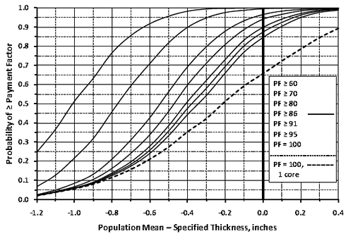
Figure 101. Graph. OC curves for PCC thickness for populations with = 0.50 inches.
Recommendations for Improving the Thickness Specification
A number of issues with this specification have been identified in the previous discussions. Some of these issues, along with some recommended changes to the acceptance plan, are presented in the following sections.
Discrete Payment Schedule
Specification 4 uses a discrete, or stepped, payment schedule where small differences in quality can result in fairly large differences in the PF received. When the true quality level of the work is close to a boundary in the stepped payment schedule, the quality estimate obtained for an individual lot may fall on either side of the boundary due primarily to chance. Depending on which side of the boundary the estimate falls, there may be a substantial difference in payment level, which may lead to disputes over measurement precision, round-off rules, and so forth. This problem can be avoided with a continuous payment schedule that provides a smooth progression of payment as the quality measure varies.
For example, suppose that a contractor is operating under the payment schedule in table 5 and that the target thickness is 10.00 inches. Furthermore, suppose that the following thickness results are obtained from a lot: 9.70, 9.48, and 9.29 inches and that the sample mean is 9.49 inches. The thickness deficiency is therefore 10.00 – 9.49 = 0.51 inches. This corresponds to a payment factor of 70 percent. If the last test result had been 9.32 inches instead, then the mean would be 9.50 inches, which is a thickness deficiency of 10 – 9.50 = 0.50 inches, resulting in a payment factor of 80 percent. This is a fairly large payment reduction for very little practical difference in the measured quality.
This problem can be resolved by using a continuous payment relationship, based on one or more equations, rather than the discrete relationship in table 5. A continuous schedule could be developed that provides essentially the same EP curve as the one for the discrete schedule currently used by the SHA. Computer simulation could be used to develop the EP curve for the continuous schedule. While no attempt was made to specifically match the payment schedule in table 5, for illustration purposes only, figure 102 shows how a continuous payment schedule might be fit to a discrete payment schedule.
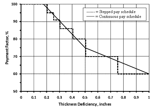
Figure 102. Graph. Continuous payment schedule fit to a discrete payment schedule.
PWL Approach
Rather than using only the sample mean, the use of PWL as the quality measure is a much better approach that incorporates both the sample mean and sample standard deviation into the payment factor determination.
The PWL approach is statistically valid, is endorsed by FHWA, has been used for decades, and has been adopted by numerous SHAs. Without the ability to determine the AQL for specification 4, it is not possible to show how a PWL specification could match the current specification requirements. However, the existing specification easily could be adapted to using PWL.
Lack of an Incentive Provision
This specification does not include an incentive provision that allows PFs greater than 100 percent. There are several arguments in favor of allowing an incentive payment for quality that exceeds the specified quality level. The most important is a matter of fairness.
Due to the random nature of the sampling process, there will be times that material at the AQL will have a sample result that indicates a reduced PF should be applied. However, if there is no incentive provision, the times when the sample result indicates quality in excess of the AQL will result in a PF of 100 percent. Therefore, it will not be possible for AQL material to receive an average PF of 100 percent.
The solution is simple. Even a relatively small incentive for work exceeding the specified AQL will correct this situation. In all cases, the EP and OC curves should be constructed to confirm that the acceptance procedure is working as desired and, in particular, that the average PF at the AQL is 1.0.
Since it was not possible to determine an AQL population for this thickness requirement, it is not possible to determine the expected payment at the AQL in this example. However, the SHA should consider either defining the AQL population, or if one has been defined, it should investigate the EP and OC curves to see how the acceptance plan performs, particularly at the AQL.
Conclusions
Some of the conclusions found in the analyses of the four specifications are as follows: